PAT: A Path-Aggregation-Tree Multicast Routing
Protocol in Wireless Sensor Networks
Hui-Tang Lin1,2, Ming-Che Chen2, Wang-Rong Chang3, and Chih-Wei Lin2
1 Department of Electrical Engineering, National Cheng Kung University, Taiwan (R.O.C.)
2Institute of Computer and Communication Engineering, National Cheng Kung University, Taiwan (R.O.C.) 3ICT-Enabled Healthcare Program, Industrial Technology Research Institute-South, Taiwan (R.O.C.)
E-mails: 1,2{htlin, q3895112, q3693104}@mail.ncku.edu.tw; 3[email protected];
Abstract―Wireless Sensor Networks (WSNs) make pos-sible many new applications in a wide range of application domains. Many of these applications are based on a many-to-many communication paradigm in which multi-ple sensor nodes send their sensed data to multimulti-ple sinks. To support these many-to-many applications, this paper proposes an energy-efficient transport protocol in which each source sensor evaluates the multicast costs of various potential multicast trees between it and the destination sinks and then selects the tree with the minimum commu-nication overhead. The simulation results demonstrate that the proposed multicast routing algorithm yields a significant reduction in the total energy consumption, and therefore enables a notable improvement in the network lifetime.
Index Terms―WSN; Multicast; Many-to-Many Communi-cation.
I. INTRODUCTION
In Wireless Sensor Networks (WSNs), the energy required by the sensor nodes to carry out their sensing, processing and communication tasks is generally provided by an on-board battery. How-ever, in many applications, it is invariably impossi-ble to retrieve the sensors once they have been de-ployed to replace the batteries. Thus, the sensors have a finite life. Therefore, when designing and implementing routing protocols in WSNs, one of the most crucial requirements is to minimize the total energy consumption in order to extend the overall network lifetime.
Various energy-efficient unicast protocols have been proposed in recent years. For example, a data-centric routing protocol, designated as Sensor Protocols for Information via Negotiation (SPIN),
was reported in [1], in which each sink sends a re-quest describing the data it requires from a speci-fied set of sensor nodes whenever it receives adver-tisements from these sensors. Similarly, in [2], the authors proposed a Direct Diffusion (DD) data-centric routing protocol which enables a sink to collect data with specific attributes from sensor nodes by setting up a communication tree. However, whilst both protocols perform well in WSNs in the sense that they can discover the shortest end-to-end path from the source sensor to each sink, they are not readily applicable to sensor applications with a many-to-many communication paradigm since each node consumes a significant amount of energy in transmitting its sensed data to the multiple destina-tion sinks on a sink-by-sink basis [3].
To resolve this problem, the current study de-velops a multicast routing protocol, called Path-Aggregation-Tree multicast routing (PAT), to identify a suitable (e.g., minimal cost) multicast routing path between the source sensor and the multiple destination sinks within the network. PAT enables the source sensors to construct various po-tential multicast trees. The total energy consump-tion can be reduced by utilizing a Multicast Cost Estimation (MCE) scheme to estimate the multicast costs of various potential trees and choose the tree with the minimum communication overhead for multicast routing purposes. The simulation results confirm that the proposed multicast routing algo-rithm yields a substantial reduction in the energy consumed by each sensor node, and therefore achieves a significant improvement in the network lifetime.
(a) (b)
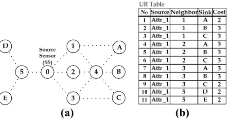
Fig. 1. (a) Illustrative example of WSN topology. (b) Corresponding UR table for Node 0.
The remainder of this paper is organized as fol-lows. Section II reviews the related studies within the literature and briefly highlights the issues aris-ing when implementaris-ing multicast routaris-ing schemes. Section III introduces the proposed multicast rout-ing protocol. Section IV presents the simulation results. Finally, Section V draws some brief con-clusions.
II. RELATED WORK
In WSNs, many geographic-based multicast
routing protocols (e.g., Minimum Incremental Power (MIP) algorithm [4], Localized En-ergy-efficient Multicast Algorithm (LEMA) [5], Geographic Multicast Routing (GMR) protocol [6], and so on) have been previously proposed to realize multicast transmissions in WSNs. Although these protocols perform multicast transmission abilities for WSNs with many-to-many communication paradigm, the costs incurred in implementing these protocols were somewhat high since the sensor nodes were required to exchange and maintain a significant amount of additional information (i.e., a subset of the total network topology information [4] or the locations of all the neighboring nodes [5][6]). In an attempt to resolve these problems in geo-graphic-based multicast schemes, the authors in [7][8] proposed an efficient and loca-tion-unawareness multicast protocol, designated as Branch Aggregation Multicast (BAM), which used a Unicast Routing (UR) table to construct an en-ergy-efficient multicast tree, thereby avoiding the requirement to exchange and store additional in-formation at each sensor.
The following subsections describe the basic
principles of the BAM protocol and then discuss the major issues arising when adopting this proto-col to achieve multicast routing.
A. Description of BAM
In describing the BAM protocol, the following discussions consider a simple network topology comprising six sensor nodes (i.e., Nodes 0-5) and five sinks (i.e., Sinks A, B, C, D and E), as shown in Fig. 1(a). It is further assumed that Node 0 is the current source sensor. Whenever Node 0 wishes to transmit data to the sinks in the network, it con-structs a UR table using the unicast DD routing protocol [2]. As shown in Fig. 1(b), the UR table has four fields, namely “Source Attribute”, “Neighbor Address”, “Sink Address”, and “Cost”. The “Cost” field indicates the number of hops from Node 0 to each of the destination sinks when rout-ing the data through the specified nearest neighboring node. When the UR table has been es-tablished, Node 0 executes the BAM algorithm to search for all the possible multicast routing paths between it and the sinks. For simplicity, in describ-ing the detailed steps of the BAM scheme, the fol-lowing discussions partition the BAM operational procedure into two sequential phases, namely the Best Routing (BR) table construction phase, and the Multicast Routing (MR) path selection phase. Phase I: BR Table Construction Phase
The aim of this phase of the BAM algorithm is to construct a BR table based upon the routing infor-mation within the UR table. Here, the term “best path” is defined as the routing path with the mini-mum hop-count between Node 0 and the desig-nated sink. The best paths to the various sinks are selected from amongst the possible routes specified in the UR table. For example, in the case shown in Fig. 1, Node 0 selects entries #1, #2, #5, #8, #9, #10 and #11 as the best paths and uses these entries to populate the BR table, as shown in Fig. 2(a). Phase II: MR Path Selection Phase
The purpose of this phase is to establish a MR table. Note that in the BR table, the more frequently a particular neighbor appears, the greater
SourceNeighborSinkCost Attr_1 1 C 3
UR Table
Attr_1 3 A 3
SourceNeighborSinkCost Attr_1 2 B 3 BR Table Attr_1 3 C 2 3 1 Attr_1 B 3 Attr_1 B 3 BestPath Attr_1 1 A 2 3 7 No 2 3 5 No 1 4 BestPath BestPath BestPath BestPath Attr_1 2 A 3 Attr_1 2 C 3 4 6 Attr_1 1 A 2 1 Attr_1 3 C 2 9 Attr_1 5 D 2 10 Attr_1 5 E 2 11 BestPath BestPath Attr_1 55 E 2 Attr_1 D 2 7 6 BR Table
SourceNeighborSinkCost Attr_1 1 A 2 1 No 1 Attr_1 B 3 2 MR Table Transferred Deleted Transferred Deleted SourceNeighborSinkCost Attr_1 2 B 3 Attr_1 3 C 2 3 Attr_1 B 3 3 5 No 4 1 Attr_1 B 3 Attr_1 1 A 2 2 1 Attr_1 5 D 2 6 Attr_1 5 E 2 7 Attr_1 1 B 3 Attr_1 3 B 3 2 8 Attr_1 2 B 3 5 (a) (b) (c) (d) Fig. 2. Illustration of basic processing steps in BAM protocol.
the number of individual node-to-sink paths which can be aggregated at this particular neighbor. For convenience, the neighbor which occurs most commonly in the “Neighbor Address” field of the BR table is referred to hereafter as the “best neighbor”. In the MR path selection phase of the BAM algorithm, Node 0 generates a MR table in accordance with the following four-step procedure.
z Step 1: Select the best neighbor from the BR table. If there exists more than one best neighbor candidate, select one candidate at random to be the best neighbor.
z Step 2: Delete the entries in the BR table whose “Sink Address” fields are the same as those of the entries associated with the best neighbor.
z Step 3: Transfer the entries associated with the best neighbor from the BR table to the MR ta-ble.
z Step 4: If the BR table still contains other en-tries, repeat the four-step procedure. Other-wise, terminate the procedure.
As shown in Fig. 2(b), three best neighbor candi-dates are discovered by Node 0 in the BR table, namely Nodes 1, 3 and 5. Assume that amongst these three nodes, Node 0 randomly selects Node 1 as the best neighbor. Since in the BR table, the
“Sink Address” fields associated with entries #3 and #4 are the same as that associated with Node 1, i.e., Sink B, Node 0 deletes entries #3 and #4 from the BR table, and then moves the entries associated with the best neighbor (i.e., entries #1 and #2 in the current example) from the BR table to the MR table. Having done so, the BR table still contains three entries, and thus Node 0 repeats the four-step pro-cedure (see Fig. 2(c)) and then finalizes the MR table (see Fig. 2(d)).
Having completed the MR path selection phase, Node 0 can start to perform multicast transmissions by following the routing paths discovered in the MR table. Figure 3(a) illustrates the corresponding multicast tree in using the MR table shown in Fig. 2(d) for multicast transmissions. As shown, this tree enables Node 0 to multicast its sensed data to neighboring Nodes 1, 3 and 5. Once Node 1 re-ceives the sensed data, it multicasts the data to Sink A and Node 4, and Node 4 then forwards the data to Sink B. Similarly, Node 3 forwards the sensed data directly to Sink C, while Node 5 multicasts the data to Sinks D and E.
B. Potential Issue in BAM
Before describing the potential issue in BAM, a performance metric is defined first to help evaluate
the performance of a multicast protocol. Let i
i
C+1
(a) (b)
Fig. 3. (a) BAM multicast tree corresponding to MR Table in Fig. 2(d). (b) Alternative multicast tree for network topology shown in Fig. 1(a). represent the multicast cost of the transmissions from the nodes in Level i of a multicast tree to their children located in Level i+1. Thus, the total mul-ticast cost (i.e., the number of hop-counts) of the multicast tree shown in Fig. 3(a), can be obtained
by summing the costs of all levels (i.e., , ,
and ) and is equivalent to + + = 1 + 3 +
1 = 5. 0 1 C 1 2 C 2 3 C C10 C12 C32
Although the BAM protocol is capable of pro-viding a multicast routing capability, there is no guarantee that the multicast tree which it discovers is the most efficient in terms of minimizing the to-tal communication cost. For instance, Fig. 3(b) presents a more energy-efficient multicast tree for the network topology shown in Fig. 1(a). In this case, the multicast tree is established by aggregat-ing the routaggregat-ing paths at Nodes 1and 5, respectively, and the corresponding multicast cost is equivalent
to + + = 1 + 2 + 1 = 4. The multicast cost
of this multicast tree is clearly lower than that of the tree derived using the BAM algorithm (see Fig. 3(a)). As a result, it is shown that the multicast so-lution provided by BAM may not be an en-ergy-efficient one. 0 1 C 1 2 C C32
III. DESCRIPTION OF PATMULTICAST ROUTING
PROTOCOL
In order to minimize the multicast cost of WSN applications based on a many-to-many communica-tion paradigm, this study proposes an effective multicast protocol, designated as Path-Aggrega-tion-Tree multicast routing (PAT). The basic prin-ciple of the PAT protocol is to evaluate and com-pare the multicast costs of all the potential multi-
Fig. 4. BNR table of SO.
cast trees which provide routing paths from the neighbors of the source sensor to the destination sinks such that the path with the minimum cost can be chosen for routing purposes. In the proposed protocol, this is achieved by using a Multicast Cost Estimation scheme, designated as MCE. Note that in describing the MCE scheme, the following dis-cussions consider the network topology and UR table shown in Figs. 1(a) and 1(b), respectively. A. Multicast Cost Estimation (MCE) Scheme
Similar to BAM, the MCE scheme makes use of the UR table constructed by the DD routing proto-col to perform estimation of the cost for each po-tential multicast tree. Whenever a source node wishes to forward its sensed data to the sinks, it consults its UR table to derive two node sets,
namely SM and SS, where SM is the set of all
neighboring nodes and SS is the set of all sinks in
the UR table.
In the UR table, the occurrence of a neighbor set having a small number of members, but providing routing paths to all the sinks in SS indicates that a
greater number of routing paths can be aggregated to this neighbor set. Therefore, the term “best neighbor-set” is introduced here to describe the
subset of SM which comprises the minimum
num-ber of neighbors, N, providing routing paths to all the sinks. Note that N lies in the range 1≤N ≤M,
where M is the total number of nodes in SM. As a
result, another parameter, SO, is further defined as a
set in which the members BB(x) comprise the best
neighbor-sets, where . In the
ex-ample shown in Fig. 1, Node 0 inspects the UR ta-ble and establishes the following parameters:
) C( 1≤x≤ M, N
(a) (b)
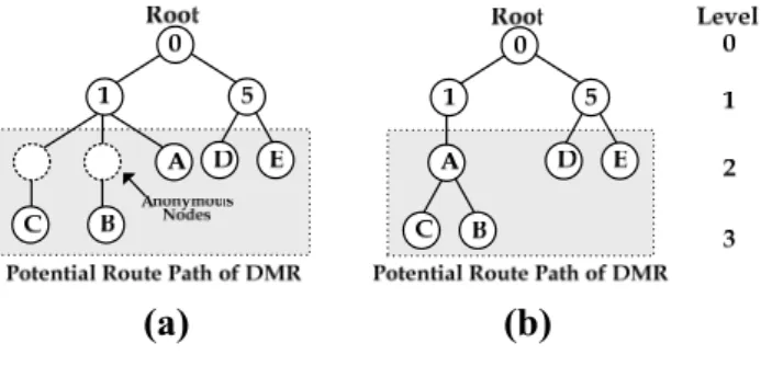
Fig. 5. (a) DMR multicast tree. (b) IMR multi-cast tree.
SM = {1, 2, 3, 5}, SS = {A, B, C, D, E}, and SO =
{BB(1) = {1, 5}, B(2)B = {2, 5}, BB(3) = {3, 5}}. (Due to the limitation of the space, further investigation on
more sophisticated schemes in determining all B(x)B
in SO is left as the future work.) Having obtained
parameter SO, Node 0 generates a Best
Neighbor-set Routing (BNR) table, as shown in Fig. 4. For each best neighbor-set, BB(x), the BNR table contains the routing information from Node 0 to all the destination sinks in the network. Note that if more than one neighbor in a best neighbor-set can reach the same sink, the neighbor with the lowest cost in the UR table is selected for inclusion in the BNR table. Furthermore, in the event that two or more neighbors in a best neighbor-set can reach the same sink and have the same cost in the UR table, the choice of neighbor is made in accordance with a random (RND) selection policy.
From the BNR table shown in Fig. 4, Node 0 is aware that there are three best neighbor-sets having the ability to relay its sensed data to all the sinks in SS. In order to determine which of the three sets is
optimum, i.e., yields the minimum multicast cost, Node 0 evaluates two potential routing scenarios for each best neighbor-set utilizing the two algo-rithms described below. Note that the following discussions take best neighbor-set BB(1) for illustra-tion purposes.
Since the BNR table only contains one-hop routing information, Node 0 has no knowledge of the forwarding paths leading from its neighbors to the sinks. For instance, in the BNR table shown in Fig. 4, Node 0 knows only that its neighbors Node 1 and Node 5 (i.e., BB(1) in SO) can act as relay nodes to send its sensed data to all the sinks in SS, i.e., it
has no idea how these two nodes actually forward the data to the destination sinks. As a result, the
source sensor (i.e., Node 0) can only predict two potential multicast routing scenarios from the nodes in B(1)B to the sinks in SN, namely:
z Disjointed Multicast Routing (DMR): In this
case, the total number of branches leading from the nodes in BB(x) (i.e., Nodes 1 and 5 in
BB(1) of the current example) is equivalent to the
number of sinks in SS.
z Integrated Multicast Routing (IMR): In this
scenario, two or more routing paths are aggre-gated at a single node and these routing paths are overlapped with the existing routing path between the source node and this node.
MCE for DMR Scenario
In order to estimate the multicast cost of the
DMR scenario for the best neighbor-set BB(1), Node
0 constructs a DMR multicast tree for B(1)B using the following DMR Multicast-tree Construction (DMC) algorithm:
z Node 0 views itself as the root and adds Nodes
1 and 5 as its children.
z Since Node 0 knows from the BNR table that
Node 1 (Node 5) has routing paths to Sinks A, B and C (D and E), it adds Nodes A, B and C (Nodes D and E) as the children of Node 1 (Node 5).
z Having completed these two steps, the total
number of branches leading from Nodes 1 and 5 in the multicast tree is equivalent to the number of sinks in the network and the dis-tance between Node 0 and each of the sinks is equal to 2 hop-counts. However, the BNR ta-ble shows that the number of hop-counts from Node 0 to Nodes B and C is equal to 3 not 2. Thus, Node 0 inserts “anonymous” nodes be-tween Nodes 1 and B and 1 and C, respec-tively.
The pseudo-code of the DMC algorithm de-scribed above is presented in Algorithm 1.
Figure 5(a) illustrates the routing paths from Nodes 1 and 5 to all the destination sinks in SS
ob-tained by applying the DMR algorithm to the best
neighbor-set B(1). Since all of the routing paths
from Nodes 1 and 5 to the destination sinks are disjointed, this DMR multicast tree can be regarded as a “worst case” routing scenario in the sense that the multicast transmission from Node 0 to all the destination sinks in the network yields the maxi-mum multicast cost, i.e., DMRB(1) =C10+ +C12 C32= 5.
MCE for IMR Scenario
Node 0 evaluates the multicast cost of the IMR scenario by establishing an IMR multicast tree for
BB(1) using the IMR Multicast-tree Construction
(IMC) algorithm described in the following:
z Node 0 views itself as the root and adds Nodes
1 and 5 as its children. Thus, the distance be-tween Node 0 and each of its neighbors in Level 1 is equal to 1 hop-count.
z Inspecting the BNR table, Node 0 finds that
the communication cost associated with Sink A when forwarding through Node 1 is equal to 2 hop-counts. Therefore, Node 0 adds Sink A to Level 2 of the multicast tree as the child of Node 1. Furthermore, the BNR table shows that forwarding data to Sinks B and C through Node 1 incurs a cost of 3 hop-counts in both cases. Therefore, in accordance with the defi-nition given above for the IMR scenario, Node 0 adds Sinks B and C to Level 3 of the multi-cast tree as the children of Sink A. In this way, the routing paths from Node 0 to B and C are aggregated at Sink A, which receives data from Node 1.
z From the BNR table, Node 0 determines that
the communication cost associated with Sinks
D and E when forwarding data through Node 5 is equal to 2 hop-counts in both cases. There-fore, Node 0 adds Sinks D and E to Level 2 of the multicast tree as the children of Node 5. The pseudo-code of the IMC algorithm presented above is shown in Algorithm 2.
Figure 5(b) illustrates the routing paths from Nodes 1 and 5 to all the destination sinks in SS
ob-tained by applying the IMC algorithm to the best neighbor-set B(1). Since in this multicast tree, the
routing paths from Node 0 to Sinks B and C are aggregated at Sink A and these paths are over-lapped with the routing path from Node 0 to Sink A, the IMR multicast tree can be regarded as the “best case” scenario, and the corresponding multicast
cost can be computed as follows: IMRB(1)=
+ + = 1 + 2 + 1 = 4. Having computed the
multicast costs of the DMR and IMR multicast trees for best neighbor-set B
0 1
C 1
2
C C32
(1), PAT computes the
equivalent costs for best neighbor-sets BB(2) and B(3)B , respectively, using an identical procedure.
B. PAT Protocol
As described above, the PAT protocol uses the MCE scheme to estimate the respective multicast costs of the worst case (DMR) and best case (IMR) routing scenarios for each of the best neighbor-sets listed in the BNR table. In the current example, the DMR and IMR multicast costs for the three best neighbor-sets listed in the BNR table in Fig. 4 are found to be: DMRB(1) = 5, IMRB(1) = 4, DMRB(2) = 6,
IMRB(2) = 4, DMRB(3) = 5, and IMRB(3) = 4.
Having obtained the worst and best case multi-cast costs for each of the best neighbor-sets, Node 0 selects the instance of BB(x) with the lowest best case
multicast cost DMRB(x) as the optimal best
neighbor-set. In the event that multiple instances of B(x)B have the same minimum best case multicast cost, Node 0 selects the instance of BB(x) with the
lowest worst case multicast cost IMRB(x) value as
the optimal best neighbor-set. If two or more best neighbor-sets have the same minimum best case and worst case multicast cost values, the optimal best neighbor-set is simply chosen using a RND strategy. In the current example, all three best neighbor-sets have the same best case multicast cost (i.e., 4 hop-counts), and thus the PAT protocol examines the respective worst case multicast cost values in order to determine the optimal best neighbor-set. It is found that best neighbor-sets B(1)B
and BB(3) have the same minimum worst case
multi-cast cost (i.e., 5 hop-counts), and thus Node 0 ran-domly selects B(1)B as the optimal best neighbor-set. The selection procedure yields the actual multicast tree shown in Fig. 3(b), in which the routing paths from Node 0 to Sinks A, B and C and from Node 0 to Sinks D and E are aggregated at Nodes 1 and 5, respectively.
The PAT scheme described above has four prin-cipal advantages. First, PAT is light weight and quite simple since the routing path discovery pro-cedure is only performed by the source sensor without additional processing at the intermediate nodes within the network. Second, since PAT ap-plies the proposed MCE scheme to evaluate poten-tial DMR and IMR routing scenarios of all of the
best neighbor-sets and then selects the best neighbor-set with the minimum communication cost, the multicast tree generated by PAT yields a lower multicast cost than that of BAM (see Figs. 3(a) and 3(b)). As a result, PAT provides a more energy-efficient solution for multicast communica-tions in WSNs. Third, PAT only makes use of the routing table constructed by the currently existed unicast routing protocols, such as SPIN [1], DD [2], etc., to derive the multicast tree; therefore, it is readily to work on top of these aforementioned unicast protocols. Finally, unlike the multicast schemes proposed in [4-6], PAT does not require the maintenance overhead of either the location in-formation of all the neighbors of each node or a subset of the total network topology. Thus, it de-mands less storage space on each sensor node. To realize multicast transmissions, the conven-tional packet header used in unicast broadcasts must be modified to include multiple receiver and sink addresses. Note that due to length constraints, the problem of designing the multicast packet header is not addressed in this study. However, in practice, PAT can be implemented using any of the multicast packet header formats proposed in the literature, e.g., the BAM header [7] [8], the DDM header [9], and so on.
IV. PERFORMANCE EVALUATION
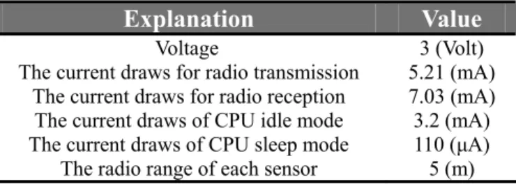
The performance of the PAT protocol was evalu-ated by performing a series of numerical simula-tions using the ns2 network simulator [10]. The simulations considered a WSN in which the sensors and sinks were randomly distributed in a 100 m x 100 m sensing field. Each sensor node was as-sumed to have a radio range of 5 m. In addition, the network traffic was modeled in accordance with a Poisson process with an average packet in-ter-arrival time of 2 (events/sec). In the simulations, the interests were periodically generated by the sinks every 10 seconds. Moreover, the wireless communications amongst the sensors and sinks were executed in accordance with the IEEE 802.15.4 protocol [11]. The sensor nodes were as-signed the same parameter settings as those used in the Power TOSSIM scheme [12] (see Table I). Finally, the problem of radio link deterioration was
0 20 40 60 80 100 120 140 2 3 4 5 6 7 8 9 10
Number of Intended Sinks per Packet (α)
T ot al E ner gy C on sum pt io n (Jo u le ) DD (β=200) BAM (β=200) PAT (β=200) DD (β=100) BAM (β=100) PAT (β=100)
Fig. 6. Variation of total energy consumption with number of intended destination sinks per generated packet.
ignored, i.e., the wireless channels were assumed to be loss free. In the simulations, the effectiveness of the PAT protocol was evaluated by comparing its performance with that of the DD and BAM routing protocols, respectively. The corresponding results are presented in Figs. 6-8, in which it is assumed that the source sensor node generates a total of 100 packets. Note that to realize a many-to-many com-munication paradigm, the generated packets are assumed to have multiple intended destination sinks.
TABLE I:SENSOR NODE PARAMETERS
Explanation Value
Voltage 3 (Volt)
The current draws for radio transmission 5.21 (mA) The current draws for radio reception 7.03 (mA) The current draws of CPU idle mode 3.2 (mA) The current draws of CPU sleep mode 110 (μA)
The radio range of each sensor 5 (m)
Figure 6 compares the variation of the total en-ergy consumption within the network with the number of intended destination sinks (α) per gener-ated packet under the PAT, BAM and DD routing schemes, respectively. Note that the figure presents results for both 100 and 200 sensor nodes, respec-tively (i.e., β = 100 and β =200). It is observed that irrespective of the protocol applied, the total energy consumption reduces as the number of sensor nodes increases. This is to be expected since the higher node density associated with a greater num ber of sensor nodes enables all three routing protocols to identify a larger number of routing paths
0 200 400 600 800 1000 1200 1400 1600 1800 2 3 4 5 6 7 8 9 10
Number of Intended Sinks per Packet (α)
Nu m be r o f F or w ar d ed Pa ck et s DD (β=200) BAM (β=200) PAT (β=200) DD (β=100) BAM (β=100) PAT (β=100)
Fig. 7. Variation of number of forwarded pack-ets with number of intended destination sinks per generated packet.
with relatively fewer hop-counts, and thus the en-ergy consumption is reduced. In addition, it is noted that for each protocol, the total energy con-sumption increases as the number of sinks per packet increases. Amongst the three protocols, the DD scheme incurs the greatest energy cost due to its use of a unicast-based transmission approach for forwarding the sensed data. Comparing the per-formance of the PAT and BAM schemes, it is evi-dent that PAT consistently achieves a lower energy consumption than BAM irrespective of the number of sensors deployed or the number of sinks per packet. The performance improvement obtained from the PAT protocol stems from the fact that on average PAT enables more routing paths to be ag-gregated at immediate sensor nodes than BAM. As a consequence, more of the individual routing paths between the source node and the destination sinks are overlapped and therefore “covered” by the same multicast transmission.
Figure 7 compares the variation in the number of forwarded packets with the number of intended sinks per packet under the three routing schemes. Since the DD protocol is incapable of transmitting a single packet to multiple sinks located on differ-ent branch paths, it inevitably results in the greatest number of forwarded packets at the intermediate nodes. Furthermore, it is observed that the PAT protocol results in fewer forwarded packets than BAM since it is specifically designed to establish a more energy-efficient multicast tree, and therefore reduces the number of forward hops required to reach the destination sinks.
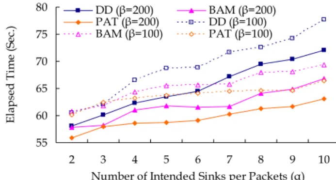
55 60 65 70 75 80 2 3 4 5 6 7 8 9 10
Number of Intended Sinks per Packets (α)
El ap se d Ti m e (S ec .) DD (β=200) BAM (β=200) PAT (β=200) DD (β=100) BAM (β=100) PAT (β=100)
Fig. 8. Variation of elapsed time required for all sinks to receive packets sent from source sensor under PAT, BAM and DD routing protocols.
Figure 8 illustrates the variation of the elapsed time required for all the sinks to receive the packets sent from the source sensor under the PAT, BAM and DD routing protocols, respectively. As shown, the DD protocol results in the greatest elapsed time since each packet is required to complete a rela-tively greater number of hops to reach the destina-tion sinks than in either the BAM or PAT routing protocols. It can also be seen that as the number of intended sinks per packet increases, the elapsed time obtained under the BAM scheme exceeds that achieved by the PAT protocol. This result reflects the fact that the PAT scheme aggregates more rout-ing paths at the intermediate nodes, and therefore reduces the total number of hops required for each packet to reach the destination sinks.
Finally, Fig. 9 shows the variation of the elapsed time before a specified number of sensor nodes fail (e.g., consume all their power). Note that in ob-taining these results, the number of intended sinks per packet was specified as 5 or 10, while the number of sensor nodes was assumed to be 200. Since the DD policy is based upon a unicast trans-mission strategy, it results in a far higher energy consumption than either the BAM or PAT schemes, and thus the nodes fail more rapidly. Comparing the two multicast routing protocols, it can be seen that irrespective of the number of intended sinks per packet, PAT yields a significant improvement in the sensor lifetime. Again, this result is to be expected since the fundamental principle of the PAT scheme is to use the MCE algorithm to identify the multi-cast tree which yields a much lower communica-tion cost. By contrast, the BAM scheme simply re-
0 100 200 300 400 500 600 700 20 40 60 80 100 120
Number of Nodes Failure
El ap se d T im e ( Se c. ) DD (α=10) BAM (α=10) PAT (α=10) DD (α=5) BAM (α=5) PAT (α=5)
Fig. 9. Variation of elapsed time required for specified number of sensor nodes to fail under PAT, BAM and DD routing protocols.
quires the source sensor to generate a multicast tree based on a MR table consisting of the routing in-formation relating to its best neighbors. Thus, whilst BAM ensures a multicast capability, there is no guarantee that the selected multicast tree repre-sents the optimal routing path in terms of its energy efficiency.
V. CONCLUSION AND FUTURE WORK
This study has presented a Path-Aggregation
-Tree multicast routing protocol, designated as PAT, for enabling multicast transmissions in WSNs with a many-to-many communication paradigm. In PAT, a Multicast Cost Estimation (MCE) scheme is used to evaluate the worst and best case routing scenar-ios for each of the identified best neighbor-sets of the source node. Having executed the MCE scheme, PAT selects the best neighbor-set which aggres-sively reduces the multicast cost and therefore yields a highly energy-efficient routing path be-tween the sensor node and all the destination sink nodes in the network. The results of a series of nu-merical simulations have shown that PAT achieves a lower communication cost, a longer network life-time, and a more rapid packet delivery service than the DD or BAM routing protocols. As a result, PAT is an ideal solution for a wide range of real-time sensing applications that are based on a many-to-many communication paradigm, including battlefield surveillance, chemical attack detection, wildfire detection, and so on.
ACKNOWLEDGEMENT
The authors would like to thank the National
Science Council, Taiwan, R.O.C., for supporting this research under grant NSC 97-2221-E-006-175 -MY3.
REFERENCE
[1] W. R. Heinzelman et al., “Adaptive Protocols
for Information Dissemination in Wireless Sensor Networks,” in Proc. ACM MobiCom, pp.174-185, Aug. 1999.
[2] C. Intanagonwiwat et al., “Directed Diffusion
for Wireless Sensor Networking,” IEEE/ACM Transaction on Network, vol. 11, no. 1, pp. 2-16, Feb. 2003.
[3] P. Ciciriello et al., “Efficient Routing from
Multiple Sources to Multiple Sinks in Wireless Sensor Networks,” in Proc. European Work-shop on Wireless Sensor Networks, Jan. 2007.
[4] J. E. Wieselthier et al., “Energy-Efficient
Broadcast and Multicast Trees in Wireless Networks,” Mobile Networks and Applications, vol. 7, issue 6, pp.481-492, Dec. 2002.
[5] J. A. Sanchez et al., "LEMA: Localized
En-ergy-Efficient Multicast Algorithm based on Geographic Routing," in Proc. IEEE LCN, pp.3-12, Nov. 2006.
[6] J. A. Sanchez et al., “Bandwidth-Efficient
Geographic Multicast Routing Protocol for Wireless Sensor Networks,” IEEE Sensor Journal, vol. 7, no.5, pp.627-636, May 2007.
[7] A. Okura et al., “BAM: Branch Aggregation
Multicast for Wireless Sensor Networks,” in Proc. IEEE MASS, Nov. 2005.
[8] A. Okura et al., “Branch Aggregation Multicast
(BAM): An Energy Efficient and Highly Compatible Multicast Protocol for Wireless Sensor Networks,” IEICE Transaction on In-formation and Systems, vol. e89-d, no. 5, pp. 1633-1643, May 2006.
[9] L. Ji et al., “Differential Destination
Multi-cast-A MANET Multicast Routing Protocol for Small Group,” in Proc. IEEE INFOCOM, vol. 2, pp. 1192-1202, Apr. 2001.
[10] Network Simulator Version 2 (ns2) Home.
http://www.isi.edu/nsnam/ns/
[11] IEEE 802.15.4 Standard Home.
http://www.ieee802.org/15/
[12] V. Shnayder et al., “Simulating the Power
Consumption of Large-Scale Sensor Network Applications,” in Proc. ACM SenSys, pp. 188-200, Nov. 2004.