A DKPHBT Based Key Management Mechanism in Heterogeneous Wireless
Sensor Networks
*ChihHung Wang and ShihYi Wei
Department of Computer Science and Information Engineering
National Chiayi University, Taiwan, R.O.C.
*whangch@mail.ncyu.edu.tw
Abstract
In the security of wireless sensor network, the most important problem is how to distribute keys for the sensor nodes to establish a secure channel in an insecure environment. Because the sensor node has limited resources, for instance, low battery life and low computational power, the key distribution scheme must be designed in efficient manner. Recently many studies added a few highlevel nodes into the network, which called the Heterogeneous Sensor Network (HSN), and made some experiments to show that the security and performance can be enhanced. But these studies need a higher communication overhead for negotiation among sensor nodes in intergroup session key distribution. In addition, some studies used probability key pool distribution and nonpairwise key distribution, which causes lower connectivity and lower resilience. In this paper, we employ the Deployment Knowledge with Polynomial Hash Binary Tree (DKPHBT) to design a key management mechanism in HSN. A PHBT is a binary tree, built by shifting and hashing the coefficients of a bivariate polynomial. Using PHBT, the highlevel nodes in different group can negotiate each other for a shared polynomial without communication. The mechanism we proposed can ensure that each pair of nodes can share a pairwise key with lower computational costs and communicational costs in sensor nodes. In addition, because of establishing the deterministic pairwise keys in the system, the higher resilience ability and connectivity can be achieved.Keywords: Heterogeneous Sensor Networks, Key Management Mechanism, Deployment Knowledge, Polynomial Hash Binary Tree
1. Introduction
Compared to the traditional network system, the wireless sensor network (WSN) is a special
network, which becomes popular in recent years due to the greatly potential low cost solutions to a variety of realworld challenge, and extensible network in regardless of the network topology [15].
In a hostile environment, sensor nodes need keys to protect the transmitted data through the insecure environment so that a key management mechanism must be established.
Recently many studies added a few highlevel nodes into the network [9], [5], [11], which called the Heterogeneous Sensor Network (HSN), and made some experiments to show that the security and performance can be enhanced.
In general way, except for the basic security requirements, a key management mechanism in WSN has to consider the following additional design principles:
1) Enhancing Network Connectivity.
2) Improving Resilience Ability.
3) Decreasing Memory Requirement.
4) Reducing Communication and Computation Overhead.
5) Improving Security Degree of the Distribution Model. The mathematical
scheme has to consider the secure degree in the model. For example, Du et al. used Blom’s key distribution method [13] to generate a pairwise key [16]. Since the security degree of Blom’s method is based on λdegree, if the number of compromised nodes is greater than λ+1, the key space will not be secure anymore.
6) Scalability of the Network.
Related Work. In WSN, [3] proposed a
probability key predistribution scheme. [16] proposed a scheme based on groupwise model with Blom’s pairwise key establishment and deployment knowledge of random key distribution, and [18] enhanced the resilience ability of [16] by using hexagonal deployment model. In [10], Shi et al. proposed a hash binary tree (HBT) based key
predistribution, and it reached the selfhealing property. In HSN studies, [9] proposed a polynomial pool based key management framework of multilevel heterogeneous sensor network. [11] presented a hybrid mechanism, which mixed Lion and Tiger up.
In our key management mechanism, we use the Deployment Knowledge [16] with Polynomial Hash Binary Tree (DKPHBT) to develop an efficient and secure scheme for heterogeneous sensor network. A PHBT is a binary tree [10], built by shifting and hashing the coefficients of a bivariate polynomial. Using PHBT, the highlevel nodes in different group can negotiate a shared polynomial without communication. The mechanism we proposed can ensure that each pair of nodes can share a pairwise key with lower computational and communicational costs. Because of establishing the deterministic pairwise key in the system, the higher resilience ability and connectivity can be achieved. Furthermore, the amount of memory usages in both highlevel nodes and the lowlevel nodes are very small.
2. Preliminaries
The network model poposed in this section is extended from the studies of [16] and [18], and we choose the polynomial as the pairwise key establishment method. In our method, the security is based on the degree t, or called a tsecure method, which means it will be broken if t + 1 or more nodes are compromised.
2.1. The network model
In large scale wireless sensor network, we assume that the deployment is a groupbased deployment model like [16]. But there are something different; first we assume that there are 2 level nodes in the sensor network, namely the highlevel node, which is used to be a cluster head (called CH), and the lowlevel node (called Lnode), which is the sensor node. Then we assume that few Hnodes and large amount of Lnodes are in a deployment group, and deployed at a single desired point, called deployment point like [16]. Using this deployment model, the nodes can reside at points around this deployment point by a certain PDF, and the nodes are static once they are deployed to the reside point. The density of the two level nodes fits for P (H) + P (L) = 1, where P (L) >> P (H), and H and L means the Hnode and Lnode respectively. Finally, after deployment, each Lnode will find its CH by the best Received Signal Strength Indicator (RSSI), and then the network groups are built. The
assumptions of the network are listed as follows: 1) There are total N Lnodes arranged to |D|
groups, and |LDi| Lnodes in the Di group, where 1 ≦ i ≦ |D|. The number of Hnodes in each deployment group is |H Di |. The equation |H Di | + |LDi| ≦ t holds, where t is the security degree.
2) The deployment groups can be arranged as a grid or hexagonal distribution. In this paper we mainly focus on the grid as Figure 1. And the distance between the deployment point and grid border is 2σ.
3) The resident point that means the final location of the deployed node, of the node k in the deployment group Di follows a PDF
) | , ( x y k D i
f Î ; here we use the twodimensional Gaussian distribution: ] 2 / ) ( ) [( 2 2 2 2 2 1 y) (x,
PDF x xi y yi c
c e s
ps
- + - - × =, where (x, y) is a coordinates and the σc 2 is
the variance of distribution for the nodes in node level c. The variances of different masses of different level nodes are also different.
4) Different level of nodes, have different masses, which will cause different variances. However, we can throw different level of nodes in different height by using a helicopter. Hence it can be assumed that the variances of different level are all the same. 5) After deployment, all the Hnodes can
broadcast a hello message within a large range area, so that all the Lnodes can choose an Hnode as its cluster head (CH) by the best Received Signal Strength Indicator (RSSI) [5]. And the hierarchical architecture group is built after this hello phase. In our model, the best signal represents the shortest straight distance between Hnode and Lnode.
6) Each network group has different number of Lnodes. Following the assumption 1), we also assume that there are less than t nodes in a network group, where t is the degree of security.
7) Adversary model: Adversaries can perform attacks only after the hello phase. We assume that the attack model follows the uniform distribution.
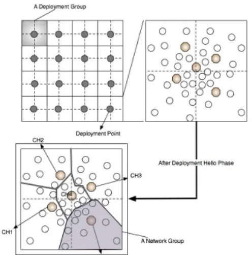
Figure 1 shows the proposed deployment model. In grid arranged deployment model, there are many deployment groups (in Figure 1 lefttop). The center of each grid is the deployment point. After deployment, the Hnodes and Lnodes
follow the PDF of twodimensional Gaussian distribution: the higher density will appear near the deployment point and the lower density will appear far away from the point (in Figure 1 righttop). In addition, we cannot predict the exact coordinates that an Hnode or an Lnode will locate. The Hnodes now become cluster heads; they broadcast hello message and then build the network topology rapidly. The final topology of network group is formed as an irregular shape, and the key management mechanism is performed for this final static model (in Figure 1 leftbottom). Figure 1. The Network and Deployment Model following twodimensional Gaussian distribution 2.2. Bivariate polynomial We choose the bivariate polynomial as our key establishment method. A bivariate polynomial like [2] is built by randomly generating its coefficients aij. We assume that the identity of each node is
unique and f(x, y) equals to f (y, x) for any x, y. The polynomial is preloaded into all CHs as a secret function. If two CHs would like to build a shared polynomial, all they needs is just shifting and hashing the coefficients of the polynomial.
3. Sketch of the DKPHBT Key
Distribution Mechanism
3.1. Design concepts
The goals of our design are described here in detail. For security consideration, we choose a pairwise key because it provides the best resilience ability; due to the node with only limited memory resource, the number of keys in a node should be as few as possible. In a pairwise key system, optimal length of a key ring is the number of neighbors of a node. Due to the advantage of the
Hnode, the key assignation and calculation should be managed by Hnodes. Because of the noninfrastructure of sensor network, apportioning all the key rings into nodes in preload phase is impossible. Hence only the master key is loaded in preload phase. And eventually, the CHs in the different group can find a cooperativefunction without communicating with each others.
To do this, we can use a random bivariate polynomial as a root polynomial to build a binary tree, and the leaves in the tree are the pairwise key generation functions, and they will be preloaded into the CHs. By using a binary tree, any two nodes in the leaf can find a lowest common ancestor, which is a polynomial, too. Finally, the ancestor node of the two CHs is the basic of their cooperativepolynomial, called copolynomial.
In secure consideration, we have to apply a oneway pseudorandom function to this tree. Since that, even if an adversary compromises a CH node and gets the polynomial, he cannot trace back the root to compromise the entire network. Although we use a oneway pseudorandom function, it may be insecure if we distribute the root to all CHs in preloaded phase.
Consequently, the main problem here is that how to distribute the leaves to CHs so that the neighboring groups can share a copolynomial but the adversary cannot compromise the whole network when only few CHs have been compromised.
In deployment knowledge, we know there are 99.7% nodes distributed in the range of 3 times of standard deviation (3σ) from the deployment point.Hence, the CH keeps only the copolynomial, which is the common ancestor with CH’s neighbor deployment groups, so that there is no need to deploy the root to the CH.
To build this Polynomial Hash Binary Tree, two methods are given here: building polynomial tree and building coefficient tree.
3.2. Building polynomial tree
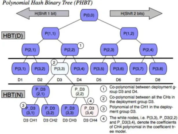
Figure 2 shows what an HBT is. HBT is a binary tree, built by hashing a value of shifting bits. We define a shift function: shiftLeft(.) and a oneway hash function: H(.). The leftchild polynomial is built by hashing the coefficients of its parent polynomial after leftshifting 1 bit, and rightchild polynomial is built by hashing the coefficients of its parent polynomial after leftshifting 2 bits. For example, P(2,1) = H(shiftLeft(P(1,1),1)) and P(2,2) = H(shiftLeft(P(1,1),2)). There are two types of HBT: one for deployment group, called HBT(D), and the
other for network group, called HBT(N). A leaf of the HBT(D) is assigned to the CHs of a deployment group, and it is the root of the HBT(N). When CHs need to get their own polynomial, they can use the leaf of HBT(D) as a new root to build the HBT(N), and the leaves of HBT(N) can be their polynomials.
Figure 2.Hash Binary Tree
In Figure 2, CH1 of a deployment group D3 can get its own polynomial P_D3(3,1). The leaf P(3,3) is also a root of HBT(N), thus it is a copolynomial for all the CHs of the deployment group D3. If the CH of D3 needs to establish a pairwise key with the CH of D4 for their member connection, they can use the copolynomial of P(2,2) of the HBT(D).
In the first method, the node of the HBT(D) consists of all the coefficients of the polynomial. HBT(D) is built as follows:
1) Define |D| as the number of deployment group, and the depth of the tree is equal to
d = log é 2 | D | ù.
2) Randomly select a bivariate polynomial defined in Session 2.2 as the root polynomial.
3) For the depth k, where
1 £ k £ d
, the left child of a node P(k,i), where i is the node number, is built byé / 2 ù ), 1 )) , 1 ( t(P
H(shiftLef k - i , and
é / 2 ù ), 2 )) ,
1 ( t(P
H(shiftLef k - i for the right child.
After extending, the leaves P(d,i) are the copolynomial of each deployment group Di. And P(d,i) is assigned to all CHs of the deployment group Di.
Then the CHs can build a HBT(N) by the copolynomial as the similar steps from 1 to 3. Let |Di| be the number of CHs of a deployment group Di and the depth d is equal to d = é log 2 | D i | ù . The HBT(N) can be built as the above step 2 and 3.
Figure 2 shows the HBT(N). After extending, the CHs of the Di can get their own polynomial from the leaves of HBT(N), and the root is their copolynomial.
After deployment, any two CHs in the same deployment group can find a copolynomial in the leaf from the HBT(D). If two neighboring CHs are not in the same deployment group, they need to share a lowest ancestor polynomial to derive their copolynomial. Since that, even if a CH is compromised and its copolynomial is revealed, the adversary cannot get all the polynomials of other deployment groups and figure out their ancestor polynomial.
3.3. Building coefficient tree
There is another way to build this HBT. Instead of randomizing and hashing the whole coefficients of a polynomial, we can build the tree by hashing only one coefficient in a time. In this method, each node is a coefficient of a polynomial, if a CH need to get its polynomial, it needs to collect a path from the leaf of its ID to the tree root, and the polynomial can be built by these coefficient nodes.
In the second method, the HBT(D) is built as follows:
1) Define |D| as the number of deployment group, and the depth is denoted by d. 2) Randomly select a number c as a root
coefficient.
3) For the depth k, where 1 £ k £ d , the left child of a node P(k,i), where i is the node number, is built by
é / 2 ù ), 1 )) , 1 ( t(P
H(shiftLef k - i , and
é / 2 ù ), 2 )) ,
1 ( t(P
H(shiftLef k - i for the right
child..
4) After extending, the leaves are the root coefficients of the copolynomials for deployment groups. And we can assign each root coefficient P(d,i) to CHs, which belong to a deployment group Di.
Now HBT(N) can be built for each network group in Di:
1) Set a security degree t, and the depth di of
the polynomial tree for deployment group Di is ú ú ú ù ê ê ê é 2 2 t .
2) For the depth k, where 1 £ k £ d i, the left
child of a node P(k,i), where i is the node number, is built by H(shiftLeft(P(k - 1, i /2
é ù
),1)) , and H(shiftLeft(P(k -1, i /2é ù
),2)) for the right child.3) After extending, the CH in the Di can get a polynomial by tracing the HBT(N) from leaf to the root of HBT(N). The root of the HBT(N) is the first of coefficients of the polynomial, represented as a[0][0], and the next node is a[1][0], and so on. We only need to build HBT(N) with a half of coefficients because a[i][j]=a[j][i], hence we can get total t*t coefficients of a bivariate polynomial.
After deployment, the copolynomial of a deployment group is made by the root of the HBT(N). For a required security degree t, the CHs can find depth d =
ú ú ú ù ê ê ê é 2 2 t , and use
H(shiftRight(root,1))d times to build the copolynomial of the deployment group Di. Due to the possibility of two CHs in neighbor but not in the same deployment group, we can find the lowest ancestor coefficient node ci,j of leaf neighbors in HBT(D), and extend the polynomial by H(shiftRight(ci,j,1))d times which required for security degree. Obviously, the second method gets less memory requirement.
3.4. Using deployment knowledge with PHBT
Obviously, the security of the network has no concern with sensor nodes due to using the polynomial pairwise key method. But the resilience ability for the CH node needs to be discussed if the CH node is assumed to be able to be compromised.
Figure 3. Deployment Knowledge and Tree Traversal
To reduce the number of compromised polynomials when a CH is captured, the height of the ancestor node of any two deployment groups should be as low as possible. To do this, we should set the neighbor leaves of an HBT(D) into the neighbor deployment groups as tight as possible. We can assign numbers to the leaves of HBT(D) from left to right for the deployment groups D1, D2… Dd by a mapping algorithm. Let di denote the
ID of polynomial assigned to Di. The goal is to find an optimal algorithm for finding the minimal value of the maximum difference between
deployment groups: } , of neighbor a is and D, , | | MAX{| MAX_D j i i j j i j i d d d d d d d d ¹ Î " =
By using the deployment knowledge, we only need to deploy the lowest ancestor among the neighbors instead of deploying the root to all CHs.
An efficient algorithm is roughly described below (demonstration by Figure 3):
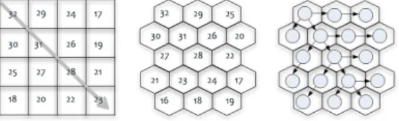
1) As Figure 3, there are 16 deployment groups in the grid model and 17 deployment groups in the hexagonal model. The depth of HBT(D) is less than 5, and we can build a HBT(D) with 32 leaves. Then we mark these leaves as a number from 1 to 32.
2) Assign 32 to the leftmost and top block, and the other blocks are assigned by breadthfirst traversal. The number assignment is in descending order.
3) The assignment rule is center first, then left, and right last for the traversal tree.
Figure 3 shows the result of this algorithm. For estimating the resilience ability, we can know the maximum difference among the neighbors in grid model is 28 – 19 = 9, and in hexagonal model is 24 – 17 = 7. In this example, the hexagonal model has better resilience ability than the grid model.
4.
The
DKPHBT
Based
Key
Management Mechanism
Table 1. Notations function hash way One : ) H( function tion authentica Message : ) MAC( s session in message revocation The : R s session in message update key session The : Update_MSG s. session in i node by d broadcaste number Random : n of ring key The : C nodes two of key pairwise The : j) G(i, between polynomial Co : ) , ( G of Polynomial : , G of j node The : G of CH The : CH i group network The : G nodes all of key Initial : s s , j i, i i i , × × s i i,j n n i j i i,j i i I r K y x f y) (x f n K j i j iNow we describe a key management mechanism based on DKPHBT. Table 1 shows the notations used in this mechanism. There are 3 phases in this mechanism: (1) preloaded phase: some keys and parameters are preloaded in the sensor nodes before deployment; (2) key
distribution phase: the network topology is established after deployment; (3) session key update phase: the session key is updated regularly in case of with and without revocation nodes. Finally, we discuss the scalability issue.
4.1. Preloaded phase
1) The system randomly chooses a system key KI and loads it into all nodes.
2) The system builds PHBT as described in Section 4:
1. Set the distribution mechanism as a grid or hexagonal model.
2. Calculate the depth of HBT(D), end build the tree.
3. Build HBT(N) and assign the polynomials to all CHs.
4.2. Key distribution phase
As network assumption in Section 3, the nodes are deployed by a helicopter in different height zones. After deployment, both the key distribution and network establishment start at the same time. In this phase, all transmission messages in the following steps include MAC(.) authentication information.
After deployment:
1) CHi broadcasts hello message with a nonce ri,1: <HelloMsg, ri,1 ||MAC(HelloMsg, KI,
CHi, ri,1)> to notice other nodes for its ID.
2) Lnodes ni,j chooses CHi as its cluster head
by the best RSSI (Received Signal Strength Indicator).
3) ni,j sends hello message <HelloMsg,
ri,1||MAC(HelloMsg,KI,ni,j, ri,1)> to all
neighbors and puts their ids into its neighboring list NeighborList(ni,j).
4) ni,j sends its registry message and
NeighborList(ni,j): <RegistMsg||
NeighborList(ni,j)||
MAC(RegistMsg,KI,NeighborList(ni,j),ni,j,
CHi, ri,1)> to CHi.
5) ni,j calculates the pairwise key shared with
CHi: K n CH i H ( K I , CH i ,n i,j , r i , 1 )
i,j = , and
calculates H( K I , r i, 1 ) as the new group master key KM. 6) CHi calculates: , i , , i j , , , f ( , ) ,if , , f ( , ) ,if and adds them into a key ring C . i , j i j i j i j n n i j i j i j n n i i j j K n n i i = ¹ ì = í ¹ î
, then CHi sends the key ring C i, j to ni,j.
7) Node ni,j saves the paiewise key with CHi
and the group master key for its key ring. Now all the pairwise keys are distributed successfully.
4.3. Session key update without revocation
In the session s, CHi must update the keys of whole network group. To do this, CHi just needs to broadcast a nonce ri,s, and the members of this
network group to update its key ring. The sensor nodes only needs to update the keys shared with its neighbor nodes in the same network group. If a communication between two nodes in the different network groups at session s is required, the two nodes exchange their ri,s’s to each other, and
update the session key by hashing their ri,s’s .
1) CHi chooses a nonce ri,s, and broadcasts < ri,s
||MAC(KM, ri,s)>.
2) ni,j updates K M s = H ( K M s - 1 , r i , s ) .
3) ni,j updates Ci,j :
ï î ï í ì Î " ¹ ¹ = = n n i,j s i s i n n s i n n n n j , i j i j , i j i j , i j i j , i j
i K r r i i K
j i,j i r K K , C if , ) , , ( H if , ) , ( H , , , , , , , . 4.4. Session key update with revocation
If there are some revocation nodes, CHi has to broadcast its nonce through a secure channel. That makes the nodes belonging to the revocation group get nothing about the nonce in this session.
For a revocation group Ri,s {ni,R1,…, ni,|R|} in
session s:
1) CHi chooses a nonce ri,s in session s.
2) CHi generates UpdateMsg= } {R E || } { s i, K CH CH CH s i, M 2 1 i | i i,|D i i, i
i, i,s n i,s n
n
i,s K ,r K , ,r K
r Å Å L Å
, where n i,j Ï R i , j , and Ek(.) is an encryption
function using key k. 3) CHi broadcast <UpdateMsg ||
MAC(KMi,j1,UpdatMsg, CHi)> to all nodes
in the group.
4) For each n i,j Ï R i , j , it can find CH i
i,j n
i,s K
r Å and get ri,s by using
s i j i, n n i,s K ) K n (r i i,j i i,j , CH CH R where , Ï Å Å . And then it updates its master key as H ( , , ) 1 i s M M K r K s i,s = - , and gets Ri,s..
5) Now the node ni,j can get the revocation list.
Then it will throw out all the pairwise keys with the revocation nodes in its key ring. 6) The node ni,j updates its key ring:
i,j n n i ,j i,j n n i,j n n n n j , i j i j , i j i j , i j i j , i j i K i i ,r ,r K j i,j i r K K C , if , ) ( H if , ) , ( H , , , , Î " ï î ï í ì ¹ ¹ = =
7) Steps 1 to 6 only update the key rings of CHi’s group members. Since the revocation member may be located on the border near to another group, CHi should announce the revocation members to its neighboring groups.
5. Discussions
This section analyzes some security issues.
5.1. Improving connectivity and energy consumption
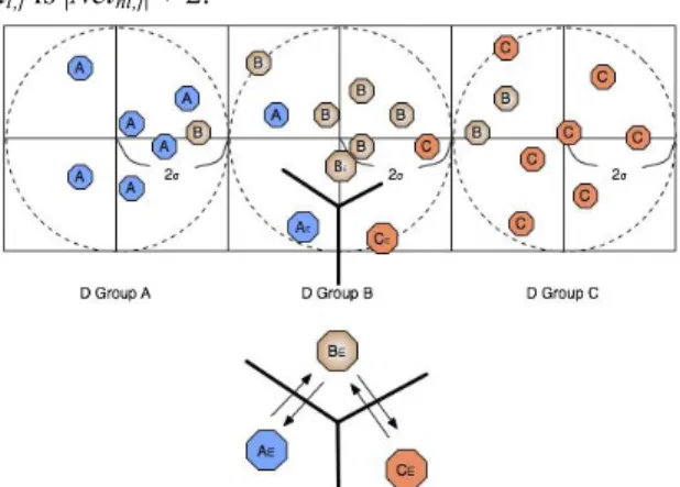
According to [3], the probability of the CH being deployed 3s out of deployment point is less than 0.3%.
Figure 4 shows what will happen with this situation. In Figure 4, the distance between the deployment point and the grid border is 2σ. Although most of CHs are deployed into the range of 3σ, some CHs such as AE and CE have no copolynomials with their neighbors. In this case, if some Lnodes are deployed into the range of AE or CE, which means they choose AE or CE as their cluster head, the Lnodes of network group AE have no pairwise keys with the Lnodes of network group CE even if they are very close to each other.
To reach secure communication, the nodes of network group AE can transfer data securely through the network group BE to the network group CE. However, this will consume extra energy.
To overcome this problem, we can assign a higher level copolynomial to CHs in preload phase, so that CHs can calculate more pairwise keys with their neighboring network groups. Due to the higher ancestor being able to derive more copolynomials of the deployment groups; the network resilience will be decreased.
Another way to solve this problem is to increase the distance between the deployment point and the grid border. For example, we can increase the distance from 2s to 2.5s. It will reduce the probability that the CH is deployed into a neighboring area.
In addition, if the CHs can connect to each other directly, they also can use cryptography system to securely exchange messages to get a new copolynomial. This can be done by the higher ability CHs. 5.2. Scalability issue In large application of wireless sensor network, the system has to add nodes or groups in run time. Due to the size of a tree being static, we can build a tree bigger than the size of deployment group at initial time. We discuss how to add Lnodes and Hnodes into the network as follows.
1) Lnodes: To add new nodes into sensor network, the nodes have to preload master keys of all CHs in the possible deployment groups. After deployment, each sensor node chooses a Hnode with best RSSI as its cluster head, and uses the master key shared with CH to register its ID and neighboring list, and then it will get its pairwise key ring. In this model, if the original number of sensor nodes is |n| and the number of additional nodes is |a|, the equation |n| + |a| ≦ t needs to hold, where t is the security degree. Otherwise, the sensor node will pick another Hnode as its cluster head.
2) Hnodes: To make the network group more scalable, we can build the HBT(N) bigger than we need at first. The remaining polynomials can be distributed to the additional Hnodes in the future. The similar method also can be used to make the deployment group more scalable.
5.3. Memory usage of Lnodes
Because the key ring of the Lnode is built by the shared keys of its neighbors after deployment. Moreover, the key ring also contains a group master key and a pairwise key shared with the CH. Assuming that |Neini,j| is the number of neighbors
of node ni,j, the memory usage size of the node
ni,j is |Neini,j| + 2.
Figure 4. The Problem of the neighboring CHs
6. Conclusions and Future Works
Compared to Du et al.’s scheme [16], we use deployment knowledge to determine the polynomial distribution for CH that can provide
better resilience for Hnodes. Due to applying the pairwise key system, both the local connectivity and global connectivity in our key management mechanism can reach near to 1. Compared with [9], [5], and [11], our method does not need extra communications for intergroup key exchange.
In the future work, we are planning to implement this mechanism with a simulator, like TOSSIM, to evaluate the performance and correctness of our network model and analyze the lower bound of security degree t. Also, applying this model to the multilevel heterogeneous sensor network and mary polynomial tree will be discussed in the future.
Acknowledgement
This work was supported in part by TWISC@NCKU, National Science Council under the Grants NSC 972219E006 003.
References
[1] Adi Shamir, ”How to Share a Secret,”
Communications of the ACM, Vol. 22, Number 11,
pp.612613, November 1979.
[2] C. Blundo, A. De Santis, A. Herzberg, S. Kutten,
U. Vaccaro, and M. Yung, “PerfectlySecure Key
Distribution for Dynamic Conferences,”
Advances in Cryptology – CRYPTO ’92, LNCS 740, pp. 471–486, 1993.
[3] Chen, YiJyun, “LocationAware Pairwise Key
Predistribution Scheme for Wireless Sensor Networks Against Colluding Attacks,” Master
Thesis of Department of CSIE, NCYU, Taiwan.
June 2007.
[4] Crossbow, “Wireless Sensor Networks,”
http://www.xbow.com/Products/Wireless_Sensor_ Networks.htm, June 2005.
[5] Firdous Kausar, Sajid Hussian, Laurence T. Yang,
Ashraf Masood,“ Scalable and efficient key management for heterogeneous sensor networks.”
The Journal of Supercomputing, Springer, vol. 45,
no. 1, pp. 4465, 2008.
[6] H. Chen, Adrian Perrig, and Dawn Song,
“Random Key Predistribution Scheme for Sensor Networks,” Proc. IEEE Symp. Security and
Privacy (S&P’ 03), pp. 197213, 2003.
[7] Laurent Eschenauer and Virgil Gligor, “A Key
Management Scheme for Distributed Sensor Networks,” Proc. ACM Conf. Computer and
Comm. Security (CCS’02), pp. 4147, Nov. 2002.
[8] Lihao Xu, Cheng Huang, ”ComputationEfficient
Multicast Key Distribution, “IEEE Tansactions
on Parallel and Distributed Systems, vol 19, No5,
pp.577587, May 2008.
[9] Lu, Kejie, Qian, Yi Hu, Jiankun, “A Framework
for Distributed Key Management Schemes in Heterogeneous Wireless Sensor Networks,”
Performance, Computing, and Communications Conference, 2006.
[10] Minghui Shi, XueminShen, Yixin Jiang, and Ghuang Lin, “SelfHealing GroupWise Key distributtion Schemes with TimeLimited Node Revocation for Wireless Sensor Networks,” IEEE
Security in Wireless Mobile Ad hoc and Sendor Networks, pp.3846, Oct. 2007.
[11] Patrick Traynor, Raju Kumar, Heesook Choi,Guohong Cao, Sencun Zhu, and Thomas La Porta, “Efficient Hybrid Security Mechanisms for
Heterogeneous Sensor Networks,” IEEE
Transactions On Mobile Computing, VOL. 6, NO.
6, pp.663677, JUNE 2007.
[12] Ross Anderson, Haowen Chan, and Adrian Perrig, “Key Infection: Smart Trust for Smart Dust,”
Proc. IEEE Int’l Conf. Network Protocols (ICNP’ 04), pp. 206215, 2004.
[13] Rolf Blom, “An Optimal Class of Symmetric Key Generation Systems,” Advances in Cryptology:
Proc. EUROCRYPT ’84, pp. 335338, 1985.
[14] Seyit A. Çamtepe and Bülent Yener, “Combinatorial Design of Key Distribution Mechanisms for Wireless Sensor Networks,”
IEEE/ACM Transactions on networking, vol 15,
No2, pp. 346358, April 2007.
[15] John Paul Walters, Zhengqiang Liang, Weisong Shi, and Vipin Chaudhary, ”Wireless sensor network security: a survey.” In: Xiao Y. (ed)
Security in distributed, grid, and pervasive computing. Auerbach Publications, CRC Press,
ISBN 0849379210.
[16] Wenliang Du, Jing Deng, Yunghsiang S. Han, and Pramod K. Varshney, “A key predistribution scheme for sensor networks using deployment knowledge,” IEEE Transactions on Dependable
And Secure Computing, VOL.3, No.1, pp.6277,
March 2006.
[17] Yun Zhou, Yuguang Fang, “Scalable and Deterministic Key Agreement for Large Scale Networks,” IEEE Transactions On Wireless
Communications VOL. 6, NO. 12, pp. 43664372,
DECEMBER 2007.
[18] Zhen Yu and Yong Guan, “A key predistribution scheme using deployment knowledge for wireless sensor networks.” IEEE Information Processing