一個基於區域色彩分布的全自動快速切割演算法

(1)

一個基於區域色彩分布的全自動

一個基於區域色彩分布的全自動快速

快速

快速切割演算法

切割演算法

研究生：陳立人指導教授：陳玲慧博士國立交通大學多媒體工程研究所碩士班摘摘摘 摘要要要要在本論文中，我們提出一快速自動切割物體的新方法。基於人類的視覺系統，我們定義出切割中所需之特徵向量。首先我們先根據區域色彩的分布情形將相似的色彩紋理樣式歸為區域。接著便分析各區域的特性：色彩組成、大小、相對位置、及粗糙程度。最後，基於若為相同物體的兩相鄰區域其有著相似特性的事實，我們將特性相似的相鄰區域合併。大部分的紋理切割研究中透過小波轉換來取得紋理的特徵來產生切割結果；然而，在自然影像中的不規則紋理通常導致其有著過度切割的問題。我們所提出的特徵向量可較有效的表示自然影像中的不規則色彩紋理，而其運算上亦較小波轉換為簡單。我們的方法能在合理時間內得到符合人類視覺的可靠切割結果。本文所呈現的實驗結果和現有的切割演算法之比較亦顯現出此法的有效性。

(2)

A Fast Automatic Segmentation Algorithm based on Local

aaaaaaaaaaaaaaa Color-Distribution

Student: Li-Jen Chen Advisor: Dr. Ling-Hwei Chen Institute of Computer Science and Engineering

National Chiao Tung University

ABSTRACT

In this thesis, we proposed a new fast method in automatic object segmentation. Based on human visual system, we define some features needed in segmentation. According to local color distribution, similar color-texture patterns are grouped into a region first. Then we analysis properties of each region: color composition, size, relative position, and coarseness. Finally, similar neighboring regions based on the fact that two neighboring regions belonging to the same object will have similar properties are merged. Most texture segmentation algorithms via wavelet transform adopt textural features to achieve segmentation proposes. However, it often has over-segmentation problem for irregular texture in natural images. Our propose feature vector can represent irregular color-texture in natural scenes. It is also computationally more feasible than wavelet transform.aOur method can generate acceptable result based

(3)

on human vision in a reasonable time. Some experiments and comparisons with some existing algorithms are also given to show the effectiveness of the proposed method.

(4)

LIST OF FIGURES

Fig. 2.1 The flowchart of the proposed method...5 Fig. 2.2 An example of Color Quantization. (a) A full color (24bit) image. (b) A

quantized image with only eight colors...9 Fig. 2.3 Examples of regional segmentation. (a)The result using window size = 15

to calculate the feature vectors. (b) The result using window size

=7...13 Fig. 2.4 An examples of region merging. (a) The regional segmentation result in

stage I. (b) The result after applying region merging on (a)...17 Fig. 2.5 An Example of Case 1 for fragments removing. (a) The enlarged partial result

in Fig. 2.4(b) with two fragments circled by red color. (b) The result after removing two fragments in (a)... 18

Fig. 2.6 An examples of Case 2 for Fragment Removing. (a) The enlarged partial result in Fig. 2.4(b) with one small fragment circled by red

color. (b) The result after removing the small fragment in (a)...19 Fig. 3.1 Image segmentation examples. From left to right: the original pictures, the

segmentation results using JSEG [4], the segmentation results using

Chen's method [2], and the segmentation results using our method... 22

Fig. 3.2 Image segmentation examples. From left to right: the original pictures, the inputs for Protiere's [5] method, the segmentation results using

Protiere's method, and the segmentation results using our method...23 Fig. 3.3 Other segmentation results using our method...24

(6)

CHAPTER 1 INTRODUCTION

1.1 Motivation

Segmentation is a method that subdivides an image into regions or objects. Segmentation can be used in many areas like: medical imaging, object location in satellite images (roads, forests, etc.), face recognition systems, automatic traffic controlling systems, and machine vision, etc. For different applications, segmentation can be divided into two subsets. Some applications like image synthesis need nearly-perfect boundary and can accept user’s involvement. This type of segmentation is called semi-automatic segmentation. Others like automatic traffic controlling system only need rough boundary and do not allow any user’s involvement. This type of methods is called automatic segmentation. In recent years, for the population of digital camera, more and more digital pictures are founded on Web. In order to manage these pictures in an effective way automatically, Content-Based Image Retrieval (CBIR) system becomes an important technique. Automatic segmentation also plays a critical rule in CBIR system.

Automatic segmentation has been a tough topic. This is due to that good segmentation needs pre-knowledge of what the “good” result is and this knowledge often needs user’s involvement. Computational

(7)

complexity is also very high in automatic segmentation, since the difficulty in modeling irregular object in natural scenes.

In this thesis, we provide an automatic segmentation method. Our method uses a low-dimensional feature vector based on local color distribution. This feature vector can represent color-texture well in a simple and intuitive way to fit human perception. This feature vector also lowers the computational complexity. Combined with other properties of human vision, such as color composition, size, relative position, and coarseness, similar feature vectors will be classified to an object that is more correspond to semantic object as perceived by human observers. The detail of our proposed method will be described in Chapter 2.

(8)

1.2 Previous Works

In 1992, Pappas [1] proposed an adaptive method for segmenting images of objects with smooth surfaces. This method is a generalization of the K-means clustering algorithm to include spatial constraints and to account for local intensity variations in the image. It uses Gibbs random field model to include the spatial constraints. Local intensity variations are accounted for in an iterative procedure involving averaging over a sliding window whose size decreases as the algorithm progresses. This algorithm outperforms the K-means algorithm. It has been quite successful for segmenting images with regions of slowly varying intensity but over-segments images with texture. The computation is heavy in computing local intensity.

In order to improve the over-segmentation problem on textured area caused by Pappas’ method, Chen [2] proposed a new segmentation method based on two types of spatially adaptive low-level features: the spatially adaptive dominant colors and the grayscale component of the texture. The performance of the proposed algorithm is demonstrated in the domain of photographic images, including low-resolution, degraded, and compressed images. This method has high computational complexity, so it cannot be used on high-resolution picture.

In 2001, Deng [3] proposed a method called “JSEG”, which consists of two independent steps: color quantization and spatial segmentation.

(9)

Colors are quantized into several representative classes, and image pixels are replaced by their corresponding color class labels, a class-map of the image is formed. The focus of this work is on spatial segmentation, where a criterion for “good” segmentation using the class-map is proposed. This method also has over-segmentation problem in textured region.

In 2006, Alexis Protiere [4] proposed an interactive method for image segmentation. This method needs user to roughly scribble different regions of interest first. It has low computational complexity, and the segmentation result depends on user’s scribbles. The more scribbles are on object especially nearing boundary, more accurate result can be obtained.

In this thesis, we present a new automatic segmentation method with low computational complexity. It can get pretty good result especially in color-texture region.

1.3 Organization of the Thesis

This thesis is composed of four chapters. In Chapter 1, the motivation and previous works are introduced. Our proposed algorithm for automatic segmentation will be presented in Chapter 2. Segmentation results and comparisons to other approaches are presented in Chapter 3. The conclusions are summarized in Chapter 4.

(10)

CHAPTER 2 PROPOSED METHOD

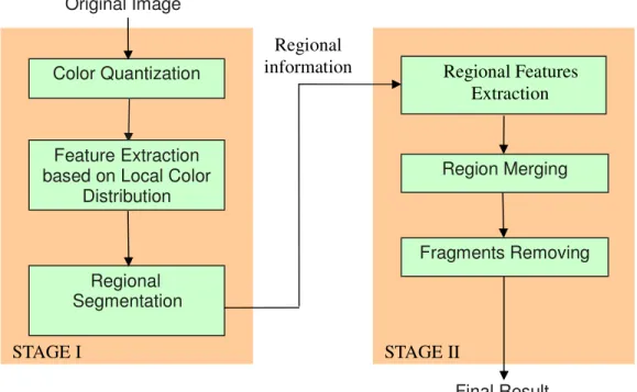
In this thesis, we propose a new method for automatic object segmentation. Based on human visual system, we define some features for segmentation. This method is composed of two stages. In the first stage, based on local color distribution, we provide a simple clustering algorithm to divide an image into several regions, each of region combines pixels with similar color-texture together. In the second stage, according to the regional information such as color composition, size, relative position, and coarseness, similar regions are merged. Fig. 2.1 shows the flowchart of the proposed method.

Fig. 2.1 The flowchart of the proposed method.

Color Quantization

Feature Extraction based on Local Color

Distribution Regional Segmentation Region Merging Final Result Original Image Fragments Removing STAGE I STAGE II Regional Features Extraction Regional information

(11)

2.1 Stage I: Segment an Image into Regions

In this stage, we want to classify an image into regions with similar color-texture. First we extract dominant colors by color quantization. Based on the quantized image, the local color distribution of a pixel is considered as a feature vector computed. And then a clustering method is provided to group neighboring pixels with similar feature vectors into regions.

2.1.1 Color Quantization

There exist thousands of colors in true color image. However, human visual system cannot recognize many colors concurrently. Color is one of the most important features when people recognize an object. In order to use color feature for segmentation, we need to merge similar colors into the same class, this work is called “color quantization.” To do color quantization, we use K-means algorithm [5] to classify all colors in the image into KC clusters; the algorithm tries to minimize the error

function shown as follows:

(1)

Where Si is cluster i, i = 1,2,...,KC and µi is the mean point of Si.

∑ ∑

= ∈

=

C i j K i x S i j

x

V

1

)

,

distance(

µ

(12)

The K-means algorithm is described as below:

1). Partition the input points into KC initial random sets.

2). Calculate the centroid (mean point), of each set.

3). Construct a new partition by associating each point with the closest centroid.

4). Recalculate centroids for the new clusters.

5). Repeats step 3). and 4). until each centroid is no longer changed.

There are two things we should define in K-means algorithm, i.e., distance function and number of classes.

1. Distance function:

Each color is a three-dimensional vector in RGB color space. However, RGB color space is perceptually non-linear to human vision. In this thesis, we transform RGB color space into CIELab color space [6] based on ITU-R Recommendation BT.709 using the D65 white point reference:                     =           B G R Z Y X 0.950227 0.119193 0.019334 0.072169 0.715160 0.212671 0.180423 0.357580 0.412453 ' ' ' (2)

(13)

     = = = 1.088754 / ' 000000 . 1 / ' 0.950456 / ' Z Z Y Y X X (3)     > − ⋅ = othewise Y * 903.3 0.008856 16 116 * 3 1 3 1 Y if Y L (4) * 500 ( 3) 1 3 1 Y X a = ⋅ − (5) * 200 ( 3) 1 3 1 Z Y b = ⋅ − (6)

Lab color is designed to approximate human vision. It aspires to perceptual uniformity. Based on this property, we define our distance function as follows:

(7)

where W is the weight for luminance. Here we choose W=0.5. The weight is used to lower the effect of variant lighting condition.

2. The number of classes:

With experiment, we found that eight colors can represent most pictures sufficiently. However, there are still pictures that contain more than eight dominant colors. So we need to determine the visual similarity

2 2 1 2 2 1 2 2 1 2 1 1 2 2 2 2 1 1 1 1 ) ( ) ( ) ( ) , ( D ) , , ( ) , , ( b b a a L L W C C b a L C b a L C − + − + − × = = =

(14)

using the function defined as follows: ) /( )) , ( D ( , ) , ( ) , ( 1 O Q M N E I y x y x y x × =

∑

∈ (8)

where O(x,y) is the original Lab color vector of pixel (x,y) in image I,

picture, Q(x,y) is the quantized Lab color vector of pixel (x,y), M is the

image’s height and N is the image’s width. Based on our experiment, when E>6, the quantized image cannot represent the original image sufficiently. Therefore, we need to increase our number of colors KC

(initial KC=8) by one. Then repeat the color quantization step using the

new KC until E≦6. Fig. 2.2 shows an example of color quantization.

(a) (b)

Fig. 2.2 An Example of Color Quantization. (a) A full color (24bit) image.

(15)

2.1.2 Feature Extraction based on Local-Color distribution

In human visual system, human often view pixels with similar color compositions in their neighboring areas as the same region. We propose a simple feature that can represent color and some texture properties concurrently. We define a feature vector for every pixel in the image based on local dominant color distribution as follows:

(9)

where KC is the number colors in quantized image, w is the number of

points in a sliding window, ni is the number of points belonging to

quantized color class i in the sliding window centered at the pixel. Briefly speaking, we consider the probability for every quantized color class occurring in the sliding window as the pixel’s feature. The defined feature vector has following advantages:

1. Our propose feature vector can represent irregular color-texture in natural scenes. There are rich color and texture in natural scenes. Most texture segmentation algorithms via wavelet transform adopt textural features to achieve segmentation proposes. Since the characteristics of the pixels in a texture region are not similar everywhere from a global view point, over-segmentation often

w

n

f

F

i i K_C

/

)

,...,

,

(

₁ ₂

=

(16)

occurs for a natural image. Our propose feature vector can perform better in irregular texture.

2. The feature vector has lower dimensions. This makes later computation much faster.

3. Feature computation is simpler than those methods [1], [2] that need to compute other local information like averaging the colors of the pixels in each class over a sliding window as feature vector. It is also computationally more feasible than wavelet transform.

There is another critical factor regarding the size of sliding window chosen. It must be large enough to capture the local color distribution characteristics, but the object boundary should not be covered. Our experiments indicate that using window size = _ _

20 width s image'

can get

pretty good result in most cases.

2.1.3 Regional Segmentation

Regional segmentation simply uses the feature defined in Section 2.1.2 to classify every point in the image by K-means clustering algorithm. The distance function is defined as follows:

(10)

∑

− = = = c C K C K K i i f f ,F F f f f F f f f F 2 2 1 2 1 2 2 2 2 2 1 1 1 1 ) ( ) ( D ) ,..., , ( ) ,..., , ( 2 1 2 1

(17)

where 1

F and 2

F are two local-color distribution feature vectors in the image.

There remains one unknown parameter, the number of classes in image, K, in regional segmentation. We set K = 4. After applying K-means clustering, we will check each point P. Let F be the feature vector of P, and:

D=D₂(F,C) (11)

where C is the feature centroid of the cluster that P belongs to. If D > D0,

then we consider P is misclassified. The threshold D0 is set to be

C K × 1 . 0 here.

For any class, if there are more than 15% misclassified points, we conclude that this class may contain more than one significant pattern and need to be reclassified. So we reclassify such a class into two new classes by K-means algorithm. We repeat this step until no class contains more than 15% misclassified points. Fig. 2.3 shows two examples of the regional segmentation:

(18)

(a) (b)

Fig. 2.3 Examples of regional segmentation. (a)The result using window

size=15 to calculate feature vectors. (b) The result using window size=7.

2.2 Stage II: Merging regions into objects

In the previous stage, we combine pixels with similar color-texture properties into regions. However, an object is usually segmented into several regions (see Fig.2.3). Based on the regional information in stage one, in this stage, we analysis properties of each region: color composition, size, relative position, and coarseness. Then we merge similar regions based on human’s perception to improve the segmentation result.

2.2.1 Region’s Color Features

In this stage, for each region, R, obtained in Stage I, we first apply K-means algorithm in R to get Kdc dominate color vectors, then a feature

(19)

Q

=

{(

c

i

,

p

i

),

i

=

1 ,...,

K

dc

,

p

i

∈

[

0 ,

1 ]}

(12)

where ci is a dominant color vector in R, pi is the percentage of ci

occurring in R, andK_dc =K_c/2. Since Kdc is the number of dominant

colors in a region, it does not need to be as many as Kc, which is the

number of dominant colors in the image. Based on our experiments, half of the Kc colors are enough to represent each region.

2.2.2 Regions’ Color Distance

Here, we adopt Chen’s method [2] to define the color distance measurement between two regions. Chen [2] provided a color distance measure based on the fact that two similar regions may have similar dominant colors and corresponding probabilities. The distance measure [2] is described as follows:

Let 1

Q and 2

Q are the color feature sets of two regions.

} ,..., 1 ), , {( 1 1 1 dc n n p n K c Q = = , Q2 ={(c_n2,p_n2),n=1,...,K_dc}, total_distance=0 1) Select a pair of two closest colors in 1

c and 2 c ,called 1 i c and 2 j c , where 1 i p and 2 j

(20)

2) Add distance( 1 i c , 2 j c ) min( 1, 2) j i p p × to total_distance. 3) Set     > − = = < − = = 2 1 2 1 1 2 2 1 1 2 2 1 , 0 , 0 j i j i i j j i i j j i p p if p p p p p p if p p p p

4) Repeat steps 1) to 3) until all 1

i

p and p2_j in 1

F and F2 are

equal to zero

Finally, the total_distance is the color distance between two regions.

2.2.3 Region’s coarseness

In order to prevent coarse regions from combining with smooth regions. We use variance for each region to measure its coarseness, coar, as follows: 2 region y x, y) (x, - )] [(L 1

_∑

∈ = µ R coar (13)

Where R is the number of points in the region and L(x,y) is the L value of

pixel (x,y) in Lab color space.

2.2.4 Merging between two regions

Based on the color feature set and coarseness of each region, we can merge similar regions together. For every region, first we check each of

(21)

its ‘neighboring regions.’ If the color distance between the region and its neighboring region is less than threshold Tc=12 and their coarseness

difference D_v defined as follows is less than 100, they will be merged.

Dv = coar1−coar2 (14)

where coar₁ and coar₂ are the coarseness for two regions respectively.

The merging step is repeated until no two regions fit the merging criterion. Fig. 2.4 shows an example of region merging:

(a) (b)

Fig. 2.4 An example of region merging. (a) The regional segmentation

result in stage I. (b) The result after applying region merging on (a).

2.2.5 Fragments Removing

From Fig. 2.4(b), we can see that there still exist some small regions (called fragments here). These fragments could be some small parts of an

(22)

object (e.g. eyes or nose) or noises caused by luminance variance. They usually have significant difference in color-texture with their neighbors, however, each of these fragments is too small such that it can not be a single object. In this section, we induce a method to remove these fragments by merging them into their neighboring regions.

We first define two types of fragments and then describe the corresponding removing processes, respectively.

Case 1: Fragment with only one neighbor

When a fragment, Rs, has only one neighbor, Rn, we check the

following inequality:

A_s/A_∆ <0.05 (15)

where As is the area of Rs, and A∆ is the area of Rn. If inequality (15) is

satisfied, Rs is merged into Rn. An example is given in Fig. 2.5.:

Case 2: Small Fragments with more than one neighbor

We now want to remove those small fragments with more than one neighbor. Below is our definition of “small”:

(23)

(a) (b)

Fig. 2.5 An Example of Case 1 for fragments removing. (a) The enlarged

partial result in Fig. 2.4(b) with two fragments circled by red color. (b) The result after removing two fragments in (a).

A_s/(M× N)<0.01 (16)

where A_s is the area of the fragment, M is the image’s height and N is

the image’s width. For every small fragment, we merge it to one neighbor which has the closest color distance. We repeat this step until there is no small fragment in the picture. One example is shown in Fig. 2.6:

(a) (b)

Fig. 2.6 An examples of Case 2 for Fragment Removing. (a) The enlarged

partial result in Fig. 2.4(b) with one small fragment circled by red color. (b) The result after removing the small fragment in (a).

(24)

After dealing with all fragments in the image, we now get the final segmentation result. In next chapter, segmentation results and comparisons to other approaches are presented.

(25)

CHAPTER 3 EXPERIMENTAL RESULTS

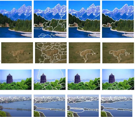
In this chapter, we will show our segmentation results and comparisons to other approaches. In Fig. 3.1, the left most pictures are the original pictures cut from [2]; the second column from left are the JSEG [3] results got from [2]; the third column from left are the final segmentation results using Junqing’s algorithm got from [2]; and the right most column are the results using our method. Comparing to Chen’s [2] method and Deng’s [3] method, we have a better performance in color-texture region. In the first row of Fig. 3.1, we can see that our method obtain better boundary of mountain than others, and no over-segmentation effect occurs inside the mountain. In the forest part, JSEG does obvious over-segmentation and Chen’s method merges two forests together. In the second row, JSEG does also over-segmentation and does not sketch the leopard’s boundary well; Comparing to Chen’s method, our method has more accurate result in head, feet and tail. In the third row of Fig. 3.1, our method provides better result than JSEG’s, and has similar result to Chen’s, but our method has lower computational complexity than Chen’s method. In the bottom row of Fig 3.1, our method has similar result to JSEG’s and has better result than Chen’s.

(26)

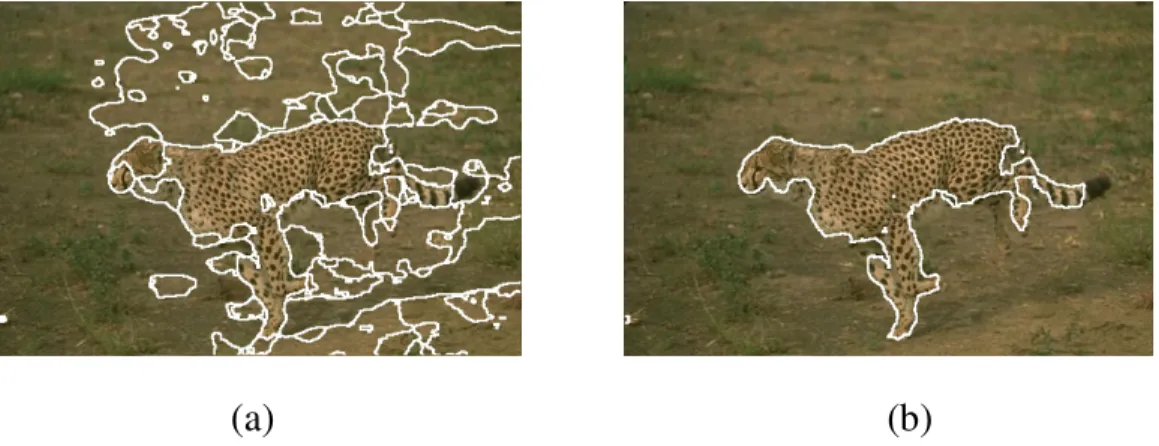
first three columns from left in Fig. 3.2 are cut from [5]; the leftmost column shows the original pictures; the second column from left shows the interactive part of Protiere’s algorithm. A user needs sketch two kinds of curves with different colors on an input image to tell where are the main object and background; the third column from left shows the segmentation results using Protiere’s algorithm; and the right most column shows the segmentation results using our algorithm. For comparison, we automatically choose the biggest object located in the center of picture as the main object and replace the other parts in the picture with black. Note that our algorithm has almost the same results as Protiere’s method. However, our algorithm does not need any user’s participation and is fully automatic.

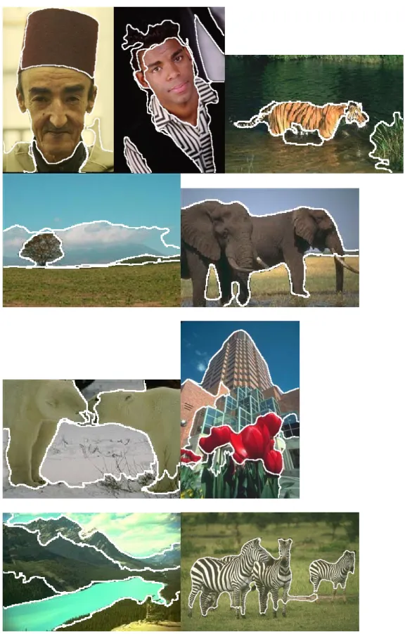
We have experimented on all test images in Berkeley Segmentation Dataset [9]. Fig. 3.3 shows some experimental results on this dataset.

(27)

`

Fig. 3.1 Image segmentation examples. From left to right: the original

pictures, the segmentation results using JSEG [4], the segmentation results using Chen’s method [2], and the segmentation results using our method.

(28)

Fig. 3.2 Image segmentation examples. From left to right: the original

pictures, the inputs for Protiere’s [5] method, the segmentation results using Protiere’s method, and the segmentation results using our method.

(29)

(30)

CHAPTER 4 CONCLUSIONS

In this thesis, we have proposed a new method in automatic object segmentation. Based on human visual system, we define features we needed in segmentation. The proposed method is composed of two stages: In the first stage, based on local color distribution, we run a simple clustering algorithm to generate regional segmentation result which combines pixels with similar color-texture together. In the second stage, according to the regional information, we analysis properties of each region: color composition, size, relative position, and coarseness. And then we merge regions belonging to the same object based on human’s perception to improve the segmentation result.

Most texture segmentation algorithms via wavelet transform adopt textural features to achieve segmentation proposes. However, it often occur over-segmentation problem for irregular texture in natural images. Our propose feature vector can represent irregular color-texture in natural scenes. It is also computationally more feasible than wavelet transform.

Our method can generate acceptable result based on human vision in a reasonable time. Some experiments and comparisons with some existing algorithms are also given to show the effectiveness of the proposed method.

(31)

aaaaaaaaaaaaaaaaaaaaaaa

REFERENCES

[1] T. N. Pappas, “An adaptive clustering algorithm for image segmentation,” IEEE Trans. Signal Process., vol. SP-40, no. 4, pp. 901–914, Apr. 1992.

[2] J. Chen, T. N. Pappas, and B. E. Rogowitz, “Adaptive perceptual color-texture image segmentation,” IEEE Trans. Image Process., vol. 14, no. 10, pp. 1524-1535, Oct 2005.

[3] Y. Deng and B. S. Manjunath, “Unsupervised segmentation of colortexture regions in images and video,” IEEE Trans. Pattern Anal. Mach. Intell., vol. 23, no. 8, pp. 800–810, Aug. 2001.

[4] A. Protiere and G. Sapiro, “Interactive image segmentation via adaptive weighted distances,” IEEE Trans. Image Process., vol. 16, no. 4, pp. 1046-1057, Apr. 2007

[5] J. B. MacQueen, “Some methods for classification and analysis of multivariate observations,” Proceedings of 5-th Berkeley Symposium on Mathematical Statistics and Probability, Berkeley, University of California Press, 1: pp. 281-297, 1967

[6] Dan Margulis, “Photoshop Lab Color: The Canyon Conundrum and Other Adventures in the Most Powerful Colorspace,” ISBN 0321356780.

(32)

important colors and similarity measurement for image matching, retrieval, and analysis,” IEEE Trans. Image Process., vol. 11, no. 11, pp. 1238–1248, Nov. 2002.

[8] C.Sun, “Fast algorithm for local statistics calculation for N-Dimensional images,” Real-Time Imaging, vol. 7, pp. 519-527, 2001.

[9] D. Martin, C. Fowlkes, D. Tal, and J. Malik, “A database of human segmented natural images and its application to evaluating segmentation algorithms and measuring ecological statistics,” Eighth International Conference on Computer Vision (ICCV'01), vol.2, pp.416, Vancouver, BC, Canada, Jul. 2001.

一個基於區域色彩分布的全自動快速切割演算法