SmartBone: An Energy-Efficient Smart Backbone
Construction in Wireless Sensor Networks
SHUN-YU CHUANG AND CHIEN CHEN
Department of Computer Science National Chiao Tung University
Hsinchu, 300 Taiwan
Wireless sensor network is a rapidly growing discipline with new technologies emerging, and new applications under development. The nodes in a wireless network generally communicate with each other along the same wireless channel. Unfortunately, sharing among wireless channels decreases network performance due to radio interfer-ence, and also raises energy consumption due to packet retransmission when interference occurs. Many topology control algorithms have been proposed to solve these problems. One widely used strategy is the backbone method. Backbone algorithms aim to reduce the backbone size. However, poor performance may be explored if only few backbone nodes are selected. Therefore, several heuristic algorithms such as SBC have been pro-posed. However, these algorithms cannot efficiently eliminate redundant nodes, and dramatically decrease performance, especially in relatively sparse networks. This study proposes a novel heuristic-based backbone algorithm called SmartBone to choose proper backbone nodes from a network. SmartBone includes two major mechanisms. Flow- Bottleneck preprocessing is adopted to find critical nodes, which act as backbone nodes to improve connectivity. Dynamic Density Cutback is adopted to reduce the number of redundant nodes depending on local area node density of network. SmartBone simulta-neously considers the balance of network performance and energy savings. Significantly, the proposed algorithm has a 50% smaller backbone size than SBC, and improves the energy saving ratio from 25% using SBC to 40% using SmartBone. Moreover, Smart-Bone improves the packet delivery ratio from 40% to 90% when the density of sensor networks becomes relatively sparser.
Keywords: backbone, topology control, distributed DFS, flow-bottleneck preprocessing,
critical nodes, density cutback, energy saving
1. INTRODUCTION
Wireless sensor network is a rapidly growing discipline with new technologies emerging, and new applications under development. Wireless sensor nodes deposited in various places can measure light, humidity, temperature, etc. and can therefore be used in applications such as security surveillance, environmental monitoring, and wildlife watch-ing [20]. A communication channel is generally shared among many sensor nodes in wireless sensor networks. Such sharing reduces the network performance due to aggra-vated radio interference. At the same time it raises energy consumption, since packet retransmission is needed when interference occurs. Moreover, the energy consumption could skyrocket if we don’t limit the number of active sensor nodes for the data relays. Topology control can be utilized to address the above problems. Topology control will remove unnecessary transmission links by shutting down radio transmission of redundant Received September 15, 2006; accepted February 6, 2007.
nodes. Nevertheless, topology control will still guarantee network connectivity in order to deliver data efficiently in a wireless sensor network.
The following criteria are typically applied to evaluate the performance of the to-pology control [1]: connectivity, energy-efficiency, throughput, and robustness. Energy consumption is the most significant issue in wireless sensor networks, since most sensors are powered by small batteries. Power supply issue is a severe limitation in sensor appli-cations, since most applications require the sensors to operate for a long time (i.e., for many years), and they can not be recharged while they are operating.
Topology control for energy-saving can be accomplished in two ways. The first method involves adjusting the radio power of the sensor nodes to maintain the proper number of neighbors [21, 22]. The second method involves turning off the radio power or performing some sleeping schedules for some redundant sensor nodes to reduce the unnecessary energy consumption [6]. At the same time, the wireless sensor networks must maintain a sufficient number of active nodes to perform data forwarding.
An effective topology control can enhance network performance by reducing inter-ference and increase network life time by saving energy. Adjusting the transmission range and reducing the number of redundant nodes are methods for achieving this goal. The first method saves less energy than the second, because adjusting the transmission range does not turn the radio off. Turning off the radio in the redundant nodes is a ra-tional idea, since nodes incur the same energy costs both in active communication and in an idle state. Estrin et al. [2] indicates that the energy consumption in the transmission and idle states are similar. However, the energy consumption of a sleeping node is 1000 times less than that of an active node [3]. This large ratio can be exploited to economize on energy. Several methods exist to reduce the number of redundant nodes such as back-bone-based [4, 6, 7, 10, 26, 27] or cluster-based algorithms [12, 13].
This study proposes a novel mechanism called SmartBone to construct a backbone. Some nodes are chosen as coordinators (i.e. backbone nodes) in the backbone construc-tion process. All nodes then can directly or indirectly communicate with other nodes via these coordinators. The coordinators form the backbone, and the non-coordinator nodes can perform sleeping schedule or turn off the radio to save the energy consumption. In this paper, we assume that the sensor nodes are lack of mobility, which is very common in most sensor network applications.
The backbone-based algorithms can be classified based on the size of the con-structed backbone. According to the backbone size, the schemes can be divided into non-constant [6, 14-17] and constant ratio schemes [4, 9, 18, 19]. The backbone size needs to be reduced to maximize the energy saving. Therefore, minimizing the backbone is normally the best policy. However, the problem of constructing a minimum backbone is equivalent to the problem of finding the minimum connected dominating set (MCDS) in the graph theory. Unfortunately, it is a classic NP-hard optimization problem. Constant ratio schemes ensure that the constructed backbone size should be bounded by a certain ratio against size of MCDS. Non-constant schemes would not have the above property.
Although minimizing the backbone size can save a large amount of energy, it also causes poor network performance due to resource competition and network congestion. Algorithms that simultaneously optimize the energy consumption and network perform-ance have been proved impossible to obtain [5]. However, a trade-off does exist between
the minimum energy cost and minimum congestion. In this study, we attempt to balance of the sustainability of energy cost and network performance.
WuLi [27] is a straightforward distributed algorithm consisting of a few rules, which aim to create a desired connected dominating set (CDS). The simplest rule is the following [28]: If a node v has two neighbors that are not neighbors themselves, then node v is added into a set C. This rule eventually generates a set C which is a CDS. The authors in [27] also discuss other local rules whose aim is to reduce the size of the domi-nating set by pruning redundant nodes. The version of the WuLi algorithm that we com-pare with in this paper is the one presented in [26], where the dominant pruningrules are generalized into a rule called Rule k. WuLi chooses the backbone nodes according to node ID and neighbor topology. Whenever the algorithm selects backbone nodes, WuLi method chooses the same backbone nodes unless the neighbor topology has been changed. It’s reasonable for mobile ad hoc networks, since the network topologies will be changed all the time as a result of the mobility. However, we assume the sensor nodes are without mobility. If we apply WuLi method to our case, it will result in the same set of backbone nodes being chosen repeatedly to relay the packets until the backbone is broken due to some of the backbone nodes running out of power. It will shorten the total network life time. However, SmartBone considers the residual energy and the coverage as the priority in the backbone nodes selection process. Therefore, the backbone nodes will keep rotating among all nodes to have a fair share of relay responsibility for all sen-sor nodes.
SBC [6] is a heuristic-based non-constant backbone construction method. It con-structs a backbone by determining which nodes should be selected as the coordinators of a backbone. SBC divides all nodes into two groups and judges within the same group whether a node is a redundant node. Redundant nodes are those that are close to each other in the same group, and that will not be chosen as coordinators. The first drawback of the SBC algorithm is its lack of a good overlap detection method. SBC cannot effi-ciently delete nodes that are very close to each other locally, because it considers the global redundancy threshold which determined the ratio of common neighbors. However, SmartBone adopts a Dynamic Density Cutback (DDC) mechanism to reduce the number of redundant nodes according to the dynamic thresholds, which is determined by local node density of network topology. In this study, node degree is used as the indicator of node density. The second drawback of SBC is its partition method. SBC partitions nodes into two groups, and picks up some nodes individually from both groups to form the backbone. Therefore, the nodes chosen from one group may be too close to the nodes chosen from the other group. The third drawback of SBC, which also exists in most of backbone methods, is its poor network performance especially under relatively sparse topology. Currently, most of the backbone methods work inefficiently in relatively sparse topology due to the lack of critical nodes awareness mechanism. That is, when choosing nodes as the backbone nodes, the methods do not consider which nodes have critical property, such as the cut points of the network or the nodes on the critical communica-tion paths. Therefore, more coordinators are needed to ensure an acceptable network per-formance such as packet delivery ratio.
However, SmartBone adopts an efficient mechanism to choose coordinators. We observe that choosing articulation points (cut points) as backbone nodes is just a rudi-mentary requirement. In this paper, we guarantee that the nodes (containing cut points)
which are on the critical communication paths will be selected as backbone nodes. Therefore, packet delivery is not restricted to only few transmission paths. Choosing nec-essary critical nodes for the backbone is useful, particularly in a relatively sparse topol-ogy which has few communication links.
SmartBone provides a general backbone solution, and can efficiently control the backbone size. The DDC feature of SmartBone can further delete many redundant nodes in a dense topology without affecting network performance. The rest of this paper is or-ganized as follows. Section 2 presents a SmartBone example, and elaborates on the de-sign of the SmartBone protocol, problems encountered in the dede-sign, and the novel way in which these problems were solved. Next, section 3 describes our simulation setup and reports the simulation results in detail. Conclusions are finally drawn in section 4.
2. SMARTBONE DESIGN
The proposed algorithm assumes that each device has the same transmission range. Hence, the connection between any pair of nodes is bidirectional. Each node needs to be prioritized to select appropriate nodes from the entire network to build up the backbone and to maintain an appropriate backbone size. The priority of nodes can be calculated in various ways. Bao and Garcia-Luna-Aceves [8] proposed some criteria for setting the priorities of nodes such as residual energy. In order to extend network life time, we do not hope that only a few nodes exhaust their power as coordinators. Therefore, an energy threshold is set. When the node’s energy is below the threshold, it can still perform the regular operations, such as sensing and processing data, but is not suitable as a coordina-tor to relay packets.
SmartBone considers two factors, namely the residual energy and the coverage. The priority is a linear combination of these two factors. The proportion of the two factors is adjusted by the network designer according to the network characteristics. The general recommended criteria are as follows. When residual energy accounts for a large propor-tion, it generally balances the power consumption of nodes in the network. For each round of backbone construction, the nodes with the superior residual energy are chosen as backbone nodes. These nodes consume energy by relaying packets, and then have lower priority than their neighbor nodes in the next round. When coverage accounts for a large proportion, it generally reduces the backbone size. Since the nodes chosen from candidates in each round are those with the largest coverage, it causes many redundant nodes to be deleted. Then, after picking out nodes with largest coverage for the backbone each round, fewer nodes are available to be selected as coordinators in the next backbone construction round. SmartBone adopts a linear combination of these two factors. Many other approaches, including the exponential form, were tried in this study. Finally, the simplest approach has been found to work best.
SmartBone is partitioned into four phases. The first phase is the Neighborhood In-formation Collection, in which the 2-hop neighbor inIn-formation of each node is gathered to support necessary operations for later steps.
The second phase is the Flow-Bottleneck Preprocessing (FlowBP), in which the whole network topology is checked, and critical nodes are identified based on the flow threshold. These critical nodes act as backbone seeds and backbone selection algorithm starts from these seeds. It is noteworthy that backbone algorithm generally starts by
electing several backbone seeds in the topology and then completes backbone construc-tion by making a sweep of the network spreading outwards from the backbone seeds. Backbone seeds choose appropriate neighbor nodes as coordinators to connect to remote nodes. Therefore, it is discussible with the selection of backbone seeds. Ideal backbone seeds should have high priority, such as high residual energy or large coverage. SBC chooses backbone seeds from an area with high node density so that more nodes can be covered. In this study, SmartBone extends the consideration advisedly. Backbone seeds are chosen based on the 2-hop neighbors’ information. After collecting neighborhood information, SmartBone performs FlowBP to choose critical nodes. Therefore, these critical nodes are especially chosen to act as the backbone seeds. Subsequently, Smart-Bone starts from these seeds. We would present the significance of the critical nodes in later section.
The third phase is the Backbone selecting procedure. Backbone node selection se-lects coordinators according to the priority determined by linear combination of residual energy and coverage. Finally, the Dynamic Density Cutback procedure is performed to remove redundant nodes based on a cutback threshold.
2.1 Neighborhood Information Collection
To ensure that the SmartBone can make the appropriate decisions, the necessary 2-hop neighbors’ information needs to be obtained. This information includes neighbors’ priority, and whether neighbors are backbone nodes. Each node collects 2-hop neighbors’ information by exchanging 1-hop neighbors’ information. Several approaches exist to obtain 1-hop neighbor information. For example, each node broadcasts hello packet pe-riodically, or neighbors’ information piggyback with the data packets. SmartBone adopts the former approach.
2.2 Flow-Bottleneck Preprocessing (FlowBP)
Backbone seeds are chosen based on the 2-hop neighbors’ information. After col-lecting neighbor information, SmartBone performs FlowBP to choose critical nodes. It is noticeable that those critical nodes contain articulation points. Then, these critical nodes are specially chosen to act as the backbone seeds. The connectivity can be improved in several ways, such as adding nodes [23], deploying MicroRouters [24], and using mov-able mobile routers [25]. SmartBone applies Flow-Bottleneck Preprocessing to ensure that critical nodes will be selected as coordinators. Critical nodes are nodes which are on the critical communication paths in the network. The critical nodes contain cut points deservedly.
SmartBone has additional communication overhead in Flow-Bottleneck Preproc-essing which other methods (ex: SBC) do not have. However, FlowBP only runs once after network deployment. Hence, the overhead of FlowBP is negligible judging against the total network lifetime. Although, the dense topology would become a relatively sparse topology due to node failure as time goes by. The FlowBP would have to run again to accommodate to the new topology in such circumstances.
As noted previously, FlowBP allows SmartBone to maintain necessary connectivity, particularly in a relatively sparse topology. FlowBP can detect the fragile part of
com-munication links, and make sure those links are includes in the backbone. The following is a detailed description of the FlowBP procedure.
2.2.1 Distributed depth first search (DDFS)
The purpose of Distribute Depth First Search (DDFS) is to find the number of dif-ferent possible paths to reach each node. DDFS extends the Depth First Search (DFS) algorithm to find N spanning trees in the network topology, where N is the number of nodes. We emulate a situation where each node of network sends a packet to the entire network through a spanning tree. Each node records its parents for each spanning trees. Number of different parents for each node gives us how many possible links to reach this node. The node with the smallest number of different parents indicates that most of the packets reach this node by a few bridges. Therefore, it’s important to identify two end nodes of the bridge as critical nodes. FlowBP has two main steps. The first step is the Distributed Depth First Search (DDFS) processing, and the second is Flow-Bottleneck checking. In the first step, the DDFS algorithm is performed on each node. The following is the data structure used, and the detailed DDFS procedure as illustrated in Fig. 1.
% The following is pseudo-code for DDFS procedure. We emulate the % operation of stack to perform distributed DFS algorithm. The data % structure of DDFS is defined as follows:
%
% PRED : the parent node ID % CHILD : the child node ID
% VISITED : has been visited or not % NEIGHBOR_LIST : 1-hop neighbor list % DISCOVER : the order of visit % NOWTIME : virtual visited order
% In the beginning, the DFS_ROOT performs DFS_ROOT_TASK() to launch % the DFS_SPANNING() procedure. If a node is DFS_ROOT, it sets PRED % as itself and notifies its 1-hop neighbors with 'DFS_VISITED' message.
PROCEDURE DFS_ROOT_TASK(): PRED := DFS_ROOT VISITED := 1 DISCOVER := 1 NOWTIME := 2 broadcast ( "DFS_VISITED" )
performs DFS_SPANNING() PROCEDURE ENDPROCEDURE
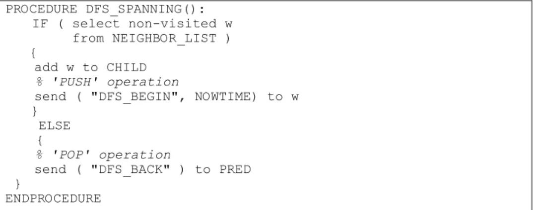
% PROCEDURE DFS_SPANNING()When node-v performs DFS_SPANNING(), it % checks whether it can choose a non-visited node-w from NEIGHBOR_LIST. % If exists such node-w then node-v notifies node-w with 'DFS_BEGIN' % message. It is equivalent to the 'PUSH' operation on the stack. % Otherwise, it equals to the 'POP' operation and node-v notifies its % parent with 'DFS_BACK' message.
PROCEDURE DFS_SPANNING(): IF ( select non-visited w from NEIGHBOR_LIST ) { add w to CHILD % 'PUSH' operation
send ( "DFS_BEGIN", NOWTIME) to w }
ELSE {
% 'POP' operation
send ( "DFS_BACK" ) to PRED }
ENDPROCEDURE
% If a node receives 'DFS_VISITED' message from node-p, it removes % node-p from its own NEIGHBOR_LIST.
PROCEDURE DFS_VISITED(): removes p from NEIGHBOR_LIST ENDPROCEDURE
% If a node receives 'DFS_BEGIN' from node-v, it's its turn to perform % DFS_SPANNING() procedure. PROCEDURE DFS_BEGIN(): PRED := v VISITED := 1 DISCOVER := NOWTIME + 1 broadcast ( "DFS_VISITED" )
performs DFS_SPANNING() PROCEDURE ENDPROCEDURE
% If node-p receives 'DFS_BACK' which send to itself from node-v, it % means that node-v finishes the exploration of spanning tree which % rooted from itself. Hence, node-p proceeds to DFS_SPANNING to explore % the remainder network topology.
PROCEDURE DFS_BACK():
performs DFS_SPANNING() PROCEDURE ENDPROCEDURE
Fig. 1. DDFS procedure.
The conventional DFS algorithm often utilizes recursion, and it generally manipu-lates the stack to simulate recursion. DDFS simumanipu-lates stack operation by sending control messages between nodes. For example, a PUSH stack operation corresponds to selecting a node from the NEIGHBOR_LIST and marking it as visited. At this moment, the visited nodes send DFS_BEGIN messages to non-visited nodes, as shown in ‘IF’ segment of Fig. 1. Conversely, a POP stack operation indicates that non-visited nodes can no longer be found in the NEIGHBOR_LIST, that is, the NEIGHBOR_LIST is null. The node with a null NEIGHBOR_LIST sends DFS_BACK message to DFS_PRED, as shown in the ‘ELSE’ segment of Fig. 1. DDFS can simulate stack operations, thus the DFS algorithm can be applied on each node in a distributed fashion.
2.2.2 FlowBP checking
The DDFS procedure is run for N times, where N represents the number of network nodes so that the information needed by FlowBP can be obtained. All nodes are then checked to determine the critical nodes. The DFS_PRED of each node is checked after repeating DDFS N times. DFS_PRED records the parent IDs of each node. If the number of different parents of one node as recorded in DFS_PRED is below or equal to a thresh-old (FLOW_TH), then the node and corresponding parent node are selected as critical nodes. Since the FlowBP can identify these critical nodes, particularly in relatively sparse topology, sufficient nodes are in the awaken state can be found to act as coordina-tors to relay packets. However, a node with large different parents under DDFS indicates that it can be reached through many possible paths. Therefore, if some of the paths are failed or obstructed, then the packets can still reach the destination node through other paths. In general, network designers deploy sensor networks with different average net-work density according to their deployment consideration. If a sensor netnet-work was de-ployed with relatively sparse topology, FLOW_TH should be higher, thus large number of critical nodes can be found. On the contrary, in dense topology, FLOW_TH is de-creased. Table 1 is the multiple levels of FLOW_TH used during our simulation. The average network density in Table 1 means the average number of neighbor nodes.
Table 1. The FLOW_TH used during simulation.
Average Network Density 20 15 10 8
FLOW_TH 0 2 5 9
In the first phase of SmartBone as we previously presented, neighborhood informa-tion is collected and recorded into the neighbor list. In the second phase of SmartBone, critical nodes are selected as backbone seeds. The backbone seeds in the network topol-ogy include the sensor gateways and the critical nodes selected via FlowBP. Subse-quently, backbone selection algorithm starts from these seeds in the third phase of SmartBone. According to the priority of nodes, some high priority nodes are picked out as backbone nodes, and some nodes are eliminated as redundant nodes via DDC. The following is the selecting and cutback procedure described in detail.
2.3 BackBone Selecting Procedure
In the backbone selecting procedure, backbone seed checks its 1-hop neighbor list, and the neighbor node with the maximum priority is picked out. However, disregarding the priority, the nodes with degree = 1 would not be the candidates for the coordinators. The reason is obvious that these kinds of nodes are on the edge of the network and can not provide relaying service to other nodes. The selected nodes are placed in the back-bone set and deleted from the neighbor list. The DDC procedure is then performed to determine whether two nodes have a redundancy relationship. At this moment, the nodes too close to the backbone node are deleted from the neighbor list. The selecting process is repeated until the neighbor list is empty and neighbor nodes are either chosen to the backbone set or deleted due to redundancy.
Subsequently, the final result of the backbone set is then broadcast to the neighbors. All 1-hop neighbors receive the message, and check whether they are in the backbone set. If a node finds itself in the backbone set, then it knows that it has been chosen as a back-bone node, and changes its state to backback-bone and starts to relay passing packets. Simul-taneously, the selected backbone nodes continue with the selecting procedure to extend the backbone as backbone seed performs the procedure described above. Conversely, if a node cannot find its ID in the backbone set, then it knows that it has not been chosen to be a backbone node. Such situation happens due to the node’s priority is not high enough, or the node itself is too close to other backbone nodes. Noticeably, regular operations of redundant nodes such as sensing and processing data can be switched on. However, their radio can be turned off to save the energy consumption. Furthermore, it is always helpful to lower the interference with proper number of nodes relaying packets. Usually a node waits for a random time period before forwarding the packet to the next hop. Too many nodes relaying packets increase the possibility of two nodes waiting for the same time slot, thus causing data collision.
2.4 Dynamic Density Cutback (DDC)
Redundant nodes must be deleted. Liu and Gupta in [6] determine whether nodes are too close to each other by checking whether the proportion of common neighbors exceeds a threshold. However, this method is not satisfactory. Decisions must be made based on the network condition. SmartBone adopts a procedure called Dynamic Density Cutback (DDC). The rules are tightened for dense topologies, meaning that more nodes are deleted (i.e., more nodes are considered too close). On the contrary, the rules are loosened for relatively sparse topologies, meaning that fewer nodes are deleted for being too close to each other, in order to maintain an acceptable network performance even under poor network conditions such as a relatively sparse topology. Multiple levels of threshold called CUT_TH are used in DDC to determine how many nodes are deleted. A CUT_TH value of n means if the number of different neighbors of two nodes is less than or equal to n, then they are too close. CUT_TH can determine the acceptable level of closeness. For instance, consider two nodes, named node-k and node-m, and k is a back-bone node. The goal is to determine whether m is too close to k. If CUT_TH is set to 0, which means if all neighbors of m are a subset of neighbors of k (i.e. the number of dif-ferent neighbors = 0), then m and k are said to be too close, and m is therefore deleted. Otherwise, m and k are not too close, and m may be chosen as the coordinator or deleted by other coordinators later. If CUT_TH is set to 2, then if m’s neighbors include more than two nodes that are not among the neighbors of node k, then m and k are not too close and hence m is chosen as the backbone node; otherwise, m and k are too close and m is deleted.
Although a sensor network is deployed with an even distribution fashion, network density could still be different from one local area to another due to the different geo-graphic areas and different ways of node deployment. Therefore, we must further define a local node density. Node degree is used as the indicator of local node density. There-fore, local node density can be easily obtained from collected neighbor information. The levels of CUT_TH values are determined according to granularity of local node density. For example, n levels indicate n − 1 local node density boundaries and n different
CUT_TH values. A larger n implies that a more detailed local node density granularity can be distinguished. In practical, we have demonstrated that choosing three levels works best, so this study uses three different local node density intervals corresponding to dif-ferent CUT_TH.
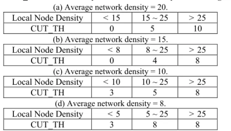
A practical example is given to explain how DDC works if network designers de-ploy sensor networks with higher average network density (e.g. the average network density = 20). Three levels were applied, and the density boundaries of these three levels can be set as 15 and 25 respectively, as shown in Table 2 (a). CUT_TH1 was therefore applied to the nodes with local node density less than 15; CUT_TH2 was applied to the nodes with local node density between 15 and 25, and CUT_TH3 was applied to the nodes with local node density more than 25. Table 2 shows the CUT_TH and local node density boundary strategy used for different average network density during simulation. Each node therefore maintains table 2 and operates DDC accordingly.
Table 2. The CUT_TH and boundary of local node density used during simulation.
(a) Average network density = 20.
Local Node Density < 15 15 ~ 25 > 25
CUT_TH 0 5 10
(b) Average network density = 15.
Local Node Density < 8 8 ~ 25 > 25
CUT_TH 0 4 8
(c) Average network density = 10.
Local Node Density < 10 10 ~ 25 > 25
CUT_TH 3 5 8
(d) Average network density = 8.
Local Node Density < 5 5 ~ 25 > 25
CUT_TH 3 8 8
A simple example is given below to illustrate the operation of SmartBone. The backbone seeds in the network topology include the sensor gateways and the critical nodes selected via FlowBP. Fig. 2 (a) shows the initial topology state. SmartBone would then perform the FlowBP procedure, which finds the critical nodes from the entire to-pology. Critical nodes are fragile components of the network structure, so they must be selected as backbone nodes. Fig. 2 (b) shows that node-d and node-e are critical nodes. The DFS_PRED of node-e is less than the threshold, so node-e and its correspondent, node-d, are chosen as critical nodes. The coordinators (including the critical nodes just selected) continue with the backbone selecting procedure, and the neighbors of the coor-dinators are considered as potential candidates for the new coorcoor-dinators. As shown in Fig. 2 (b), node-a, node-b and node-c are on the edge of the network topology, and do not help extend the backbone. Therefore, SmartBone algorithm would not choose them as coordinators. In Fig. 2 (c), assume the priorities of node-g and node-i are higher than those of other neighbors of the coordinator, so they are chosen as backbone nodes. The DDC procedure is then performed. Node-f and node-h are removed during the DDC pro-cedure because they are too close to the selected nodes, node-g and node-i. The selection procedure is continued with node-g choosing node-j until the algorithm is completed. Fig. 2 (d) displays the final result.
(a) (b)
(c) (d) Fig. 2. Example of SmartBone construction.
3. PERFORMANCE RESULTS & ANALYSIS
This study adopts the ns2 [11] network simulator to evaluate SmartBone’s per-formance. SmartBone was compared with SBC and WuLi (which adopts Rule k) based on three performance factors: backbone size, end-to-end packet delivery ratio, and en-ergy saving ratio.
3.1 Performance Metrics
Backbone size: Backbone nodes serve nodes in the network. The backbone size affects
power consumption and interference resulting from nodes sending data. These factors are closely linked to the backbone size.
End-to-end packet delivery ratio: The Packet Delivery Ratio (PDR) indicates the
backbone. The evaluating criteria of packet delivery ratio requirement differing from that of network applications are discussed later.
Energy saving ratio: The Energy Saving Ratio (ESR) was derived from dividing energy
saved by backbone methods to energy consumed by the network without backbone. The ESR indicates the energy efficiency of the algorithm. Larger ESR indicates higher energy efficiency.
3.2 Simulation Environment
The performance of SmartBone was measured with different network scenarios un-der different sets of source-destination pairs and node densities. A total of 100 nodes were random and uniformly distributed in varying topology sizes. In each topology, five transmission pairs were chosen with a simulation time of 300 seconds. To estimate ade-quately the performance of backbone construction, source and destination nodes were selected from around the topology. Information would reach the destination from the source through the backbone. In this simulation, the packet transmission interval was uniformly and randomly distributed between 0 and 0.3 seconds. Each packet size was 64 kb.
In this simulation, flooding was adopted to transmit packets between nodes. There are several reasons to choose flooding for our simulation. First, several applications need to propagate information to all nodes in sensor networks, like trigger alert notifications and query dissemination. Second, several routing algorithms still need flooding as part of the routing strategy (ex: directed diffusion). Finally, we can evaluate how the backbone reduces the collision. The following flooding parameters were applied in the simulation. To avoid collision with packets being relayed at the same time by surrounding nodes, each receiver backed off for a random time period before relaying packets again. When receiving packets, the flooding module would wait for a time interval between 0 and the maximum randomization interval, which was set to 1 second in this simulation. The probability of collision depends on the Maximum randomization interval. A larger inter-val leads to less collision, but increases the packet delay. Thus the randomization interinter-val is a trade-off. Furthermore, the Tx/Rx/Idle power was set to 660/395/35 mW according to ns2 default. The processing model did not consider the energy cost in CPU.
3.3 Simulation Results
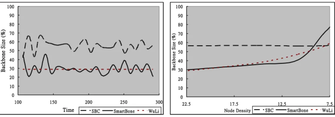
Fig. 3 illustrates how the backbone size varies with time when using the SmartBone, SBC, and CDS-based WuLi method. The topology contains 100 nodes uniform random distributed in an 800 × 800 area, and the average network density is 22.5. Significantly, the size grows and shrinks over time, except with the WuLi method. WuLi chooses the nodes according to node ID and neighbor topology. Whenever the algorithm selects backbone afresh, WuLi method chooses the same backbone nodes unless the neighbor topology has been changed. However, SmartBone and SBC choose nodes according to node priority containing residual energy and topology information. SmartBone has a backbone size of average 50% less than that of SBC, since it adopts the DDC mechanism, enabling it to delete redundant nodes more efficiently.
0 10 20 30 40 50 60 70 80 90 100 100 150 200 250 300 Time Back bone Si ze (%) SBC SmartBone WuLi 0 10 20 30 40 50 60 70 80 90 100 7.5 12.5 17.5 22.5 Node Density B ack b o n e S ize (% ) SBC SmartBone WuLi Fig. 3. Average number of coordinators elected by
the protocols during the simulation duration.
Fig. 4. Backbone size tests under different network density.
Fig. 4 illustrates the variation in backbone size for different network density, and shows that the backbone size of SmartBone is less than SBC for network density less than 9.35. Since the DDC is very effective, the backbone size of SmartBone maintains about only half that of SBC in a topology with high network density. SmartBone and WuLi methods maintain nearly the same backbone size in density topology, and it means that DDC performs as well as CDS-based method in backbone size. In a relatively sparse topology (i.e. topology with low network density > 9.35), SmartBone has a much larger backbone size than SBC and WuLi, because SmartBone addresses the importance of critical nodes. For a relatively sparse topology, more critical nodes are chosen as back-bone nodes to maintain necessary connectivity, so that in relatively sparse network con-ditions SmartBone does not degrade communication throughput. This difference is dem-onstrated in the packet delivery ratio graph below.
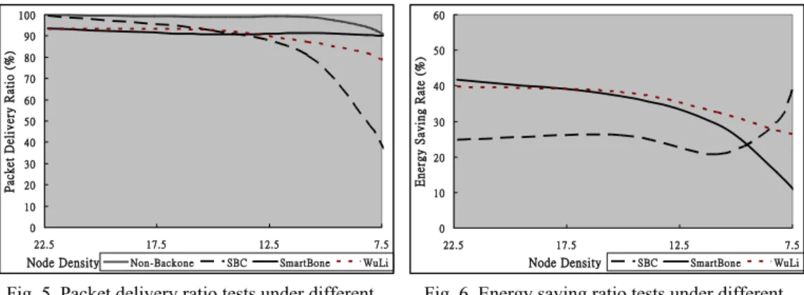
Fig. 5 illustrates the performance on end-to-end packet delivery ratio (PDR) in dif-ferent node densities. SmartBone is compared with SBC, WuLi, and WSN without a backbone (i.e. every node can relay). Non-backbone method has the highest PDR at over 90%. However, this method has the highest energy consumption as expected, since every node participates in data transmission. The PDR of SmartBone method is also over 90% for varying network density. Although the PDR of SBC is over 90% in dense topology, SBC has a much lower PDR when the network density is relatively sparse. Although, WuLi has thesimilar high PDR, it performs not as good as the SmartBone under the rela-tively sparse topology. We observe that when network density drops to 8; the SBC’s PDR is under 50% and WuLi’s PDR is under 80%. However, our SmartBone still guar-antees 90% packet delivery ratio. Since SBC does not have a critical-awareness mecha-nism, SBC has the lowest PDR in the relatively sparse networks. WuLi does not have a critical- awareness mechanism either, even though it guarantees choosing the articulation points. On the contrary, SmartBone adopts the FlowBP mechanism, which takes critical nodes in the network as coordinators. Critical nodes are very important in terms of net-work performance, especially under relatively sparse topology. The simulation shows that choosing articulation points (cut points) as backbone nodes is just a rudimentary requirement. Furthermore, SmartBone guarantees that the nodes which are on the critical communication paths would also be selected as backbone nodes.
0 10 20 30 40 50 60 70 80 90 100 7.5 12.5 17.5 22.5 Node Density Packet D eliv ery Ra tio (% )
Non-Backone SBC SmartBone WuLi 0 10 20 30 40 50 60 7.5 12.5 17.5 22.5 Node Density Energy Savi ng Rat e ( % ) SBC SmartBone WuLi Fig. 5. Packet delivery ratio tests under different
network density.
Fig. 6. Energy saving ratio tests under different network density.
The reduction in energy consumption from SmartBone, and the effectiveness of SmartBone in extending the network lifetime, was investigated. Fig. 6 illustrates the rela-tionship between network density and Energy Saving Ratio (ESR). Fig. 6 shows that SmartBone saves more energy than SBC, because it has a smaller backbone size, so more nodes are in sleeping mode. Fig. 6 also shows SmartBone saves the same amount of en-ergy as WuLi, which belongs to CDS-based method. Fig. 5 indicates that large number of sleeping nodes does not affect the network performance of PDR using SmartBone. How-ever, in relatively sparse networks SmartBone chooses more nodes as critical nodes to maintain PDR performance. Thus, SmartBone’s energy saving will be less than SBC and WuLi. In relatively sparse cases, SBC consumes the least energy. The reason is that SBC does not select critical nodes; therefore it has a smallest backbone size. A backbone is too small could decrease the available transmission paths. Therefore, the PDR of SBC drops dramatically. Because of the SBC’s PDR drops, not many packet relays happen.
3.4 Sensitivity of Thresholds
This subsection discusses the effect of network performance on different thresholds, including the Flow threshold (FLOW_TH) and Cutback threshold (CUT_TH). The net-work designer must adjust these thresholds based on the densities of netnet-work topologies, the network loading, and packet loss rate. This study provides designers with some de-sign criteria. For example, a PDR above 90% is considered to be the tolerant range. However, a PDR of 80% is acceptable for some applications, such as transferring tem-perature data. Such applications are tolerant of heavy packet loss. In such cases lower PDR is permitted.
CUT_TH is increased and FLOW_TH is decreased in dense networks, since raising CUT_TH eliminates more redundant nodes, and lowering FLOW_TH means that fewer critical nodes are selected. These two parameters help save energy by reducing the back-bone size. The opposite adjustment is performed in relatively sparse networks. CUT_TH is reduced and FLOW_TH is increased in a heavy traffic network where many backbone nodes are required to relay packets, because lowering CUT_TH means that fewer redun-dant nodes are eliminated, and raising FLOW_TH means that more critical nodes are
selected. This resembles the trade-off between energy consumption and packet delivery ratio, which gives the network designers the chance to optimize the network throughput according to their design criteria.
4. CONCLUSIONS
This study selects proper backbone nodes in wireless sensor networks using a heu-ristic-based backbone method called SmartBone. With introducing the critical-aware nodes, the SmartBone maintains a backbone with reasonable packet delivery ratios even under relatively sparse network topologies. Dynamic Density Cutback is adopted to fur-ther reduce the number of redundant nodes efficiently in SmartBone. A significant result of this study is that the proposed algorithm can achieve a 50% smaller backbone than the previous heuristic-based SBC algorithm, and improves the energy saving ratio from 25% using SBC to 40% using SmartBone. Moreover, SmartBone improves the packet delivery ratio from 40% using SBC to 90% when the density of sensor networks is relatively sparse. Furthermore, we compare SmartBone with connected dominating set (CDS) based WuLi method. The performance shows that SmartBone has a little bit smaller backbone size comparing with WuLi method. Even though WuLi and SmartBone have almost the same packet delivery ratio, however, under the sparse networks the packet delivery ratio of WuLi method is still suffering. Moreover, WuLi method suffers from shorter network life time due to the same set of backbone nodes being chosen all the time.
REFERENCES
1. R. Rajaraman, “Topology control and routing in ad hoc networks: a survey,” ACM Special Interest Group on Algorithms and Computation Theory News, 2002, pp. 60-73.
2. D. Estrin, et al., http://nesl.ee.ucla.edu/tutorials/mobicom02.
3. C. Schurgers, V. Tsiatsis, S. Ganeriwal, and M. Srivastava, “Topology management for sensor networks: exploiting latency and density,” in Proceedings of the 3rd ACM International Symposium on Mobile Ad Hoc Networking and Computing, 2002, pp. 135-145.
4. M. Min, F. Wang, D. Du, and P. M. Pardalos, “A reliable virtual backbone scheme in mobile ad-hoc networks,” in Proceedings of IEEE Mobile Ad Hoc and Sensor Sys-tems, 2004, pp. 60-69.
5. F. Heide, C. Schindelhauer, K. Volbert, and M. Grünewald, “Energy, congestion and dilation in radio networks,” in Proceedings of the 14th Annual ACM Symposium on Parallel Algorithms and Architectures, 2002, pp. 230-237.
6. H. Liu and R. Gupta, “Selective backbone construction for topology control,” in Proceedings of the 1st IEEE International Conference on Mobile Ad-hoc and Sensor Systems, 2004, pp. 41-50.
7. Y. Wang, W. Wang, and X. Y. Li, “Distributed low-cost backbone formation for wireless ad hoc networks,” in Proceedings of the 6th ACM International Symposium on Mobile Ad Hoc Networking and Computing, 2005, pp. 2-13.
8. L. Bao and J. J. Garcia-Luna-Aceves, “Topology management in ad hoc networks,” in Proceedings of the 4th ACM International Symposium on Mobile Ad Hoc Net-working and Computing, 2003, pp. 129-140.
9. K. Alzoubi, X. Y. Li, Y. Wang, P. J. Wan, and O. Frieder, “Geometric spanners for wireless ad hoc networks,” IEEE Transactions on Parallel and Distributed Systems, Vol. 14, 2003, pp. 408-421.
10. C. Sengul and R. Kravets, “TITAN: on-demand topology management in ad hoc networks,” in Proceedings of ACM SIGMOBILE Mobile Computing and Communi-cations, 2004, pp. 77-82.
11. The network simulator – NS-2, http://www.isi.edu/nsnam/ns.
12. C. C. Shen, C. Srisathapornphat, R. Liu, Z. Huang, C. Jaikaeo, and E. L. Lloyd, “CLTC: a cluster-based topology control framework for ad hoc networks,” IEEE Transactions on Mobile Computing, Vol. 3, 2004, pp. 18-32.
13. S. Srivastava and R. K. Ghosh, “Cluster based routing using a k-tree core backbone for mobile ad hoc networks,” in Proceedings of the 6th International Workshop on Discrete Algorithms and Methods for Mobile Computing and Communications, 2002, pp. 14-23.
14. B. Das and V. Bharghavan, “Routing in ad-hoc networks using minimum connected dominating sets,” in Proceedings of International Conference on Communication, 1997, pp. 376-380.
15. J. Wu and H. L. Li, “On calculating connected dominating set for efficient routing in ad hoc wireless networks,” in Proceedings of the 3rd ACM International Workshop on Discrete Algorithms and Methods for Mobile Computing and Communications, 1999, pp. 7-14.
16. I. Stojmenovic, M. Seddigh, and J. Zunic, “Dominating sets and neighbor elimina-tion based broadcasting algorithms in wireless networks,” IEEE Transacelimina-tions on Parallel and Distributed Systems, Vol. 13, 2002, pp. 14-25.
17. X. Cheng, X. Huang, D. Li, and D. Z. Du, “Polynomial-time approximation scheme for minimum connected dominating set in ad hoc wireless networks,” Technical Re-port No. TR02-003, Computer Science and Engineering Department, University of Minnesota, 2002.
18. P. J. Wan, K. M. Alzoubi, and O. Frieder, “Distributed construction of connected dominating set in wireless ad hoc networks,” in Proceedings of the IEEE Conference on Computer Communications (INFOCOM), 2002, pp. 1597-1604.
19. M. Cardei, X. Cheng, X. Cheng, and D. Z. Du, “Connected domination in multihop ad hoc wireless networks,” in Proceedings of 6th International Conference on Com-puter Science and Informatics, 2002, pp. 251-255.
20. G. J. Pottie and W. Kaiser, “Wireless integrated network sensors,” Communications of the ACM, Vol. 43, 2000, pp. 51-58.
21. R. Ramanathan and R. Rosales-Hain, “Topology control of multihop wireless net-works using transmit power adjustment,” in Proceedings of the IEEE Conference on Computer Communications (INFOCOM), 2000, pp. 404-413.
22. M. Kubisch, H. Karl, A. Wolisz, L. C. Zhong, and J. Rabaey, “Distributed algo-rithms for transmission power control in wireless sensor networks,” in Proceedings of Wireless Communications and Networking, 2003, pp. 558-563.
networks by adding nodes,” in Proceedings of the 4th Annual Mediterranean Work-shop on Ad Hoc Networks, 2005, pp. 169-178.
24. S. M. Das, H. Pucha, and Y. C. Hu, “MicroRouting: a scalable and robust communi-cation paradigm for sparse ad hoc networks,” in Proceedings of the 19th IEEE In-ternational Parallel and Distributed Processing Symposium, 2005, pp. 245.2. 25. R. Meraihi, G. Le Grand, and N. Puech, “Improving ad hoc network performance
with backbone topology control,” in Proceedings of IEEE Vehicular Technology Conference, 2004, pp. 26-29.
26. F. Dai and J. Wu, “An extended localized algorithms for connected dominating set formation in ad hoc wireless networks,” IEEE Transactions on Parallel and Distrib-uted Systems, Vol. 15, 2004, pp. 908-920.
27. J. Wu and H. Li, “On calculating connected dominating sets for efficient routing in ad hoc wireless networks,” in Proceedings of the 3rd ACM International Workshop Discrete Algorithms and Methods for Mobile Computing and Communications, 1999, pp. 7-17.
28. S. Basagni, M. Mastrogiovanni, A. Panconesi, and C. Petrioli, “Localized protocols for ad hoc clustering and backbone formation: a performance comparison,” IEEE Transactions on Parallel and Distributed Systems, Vol. 17, 2006, pp. 292-306.
Shun-Yu Chuang (莊順宇) received his B.S. and M.S. degrees
in Computer Science from National Chiao Tung University, Hsinchu, Taiwan, in 2004 and 2006, respectively. His research interests in-clude wireless sensor networks, real-time, and embedded systems.
Chien Chen (陳健) received his B.S. degree in Computer
En-gineering from National Chiao Tung University in 1982 and the M.S. and Ph.D. degrees in Computer Engineering from University of Southern California and Stevens Institute of Technologies in 1990 and 1996. Dr. Chen hold a Chief Architect and Director of Switch Architecture position in Terapower Inc., which is a terabit switching fabric SoC startup in San Jose, before joining National Chiao Tung University as an Assistant Professor in August 2002. Prior to joining Terapower Inc., he is a key member in Coree Network, responsible for a next-generation IP/MPLS switch architecture design. He joined Lucent Technolo-gies, Bell Labs, NJ, in 1996 as a Member of Technical Staff, where he led the research in the area of ATM/IP switch fabric design, traffic management, and traffic engineering requirements. His current research interests include wireless ad-hoc and sensor networks, switch performance modeling, and DWDM optical networks.