探究市場波動度資訊在技術分析中的價值 - 政大學術集成

全文

(1)國立政治大學國際經營與貿易學系博士論文. 指導教授：郭炳伸博士、林信助博士. 政治大. 立探究市場波動度資訊在技術分析中的價值. ‧ 國. 學. The Informational Role of Market Volatility Nat. n. al. er. io. sit. y. ‧. in Technical Analysis. Ch. engchi. i n U. v. 研究生：莊珮玲撰中華民國一百零二年一月.

(2) 謝辭. 本論文承蒙恩師. 郭炳伸老師與. 林信助老師不辭辛勞指導，從. 教導我如何從事研究，訓練我如何進行有系統的邏輯思考，培育我待人處事的能力，鼓勵並期許我這隻笨鳥即便慢飛，也能飛出一片屬於自我的燦爛天空。對於兩位恩師，學生謹此至上最高敬意與謝忱。感謝口試委員. 周雨田老師、蔡文禎老師及陳旭昇老師，提供. 許多寶貴的意見與對疏漏之處的匡正，使本篇論文更臻完善，謝謝老師們！. 立. 政治大. 感謝致綱學長、淯靖學姐與士真如同親人般地照顧我，給予我許. ‧ 國. 學. 多協助與建議，並鼓勵我正向思考、再接再厲、繼續努力。系上助教們有如姐姐般的關懷與協助，也令我滿心感激。謝謝你們，在此致. ‧. 上最深的謝意！. Nat. a. er. io. 先生，沒有你的支持與鼓勵，我難以成長至今。. sit. y. 最後感謝陪伴我的母親、公公、婆婆及家人們，特別要謝謝我的. n. v l 在此謹以此論文來獻給我的家人、好友及教育我的師長。 ni Ch. engchi U. 莊珮玲. 謹誌. 政治大學國際經營與貿易學系中華民國一百零二年一月.

(3) The Informational Role of Market Volatility in Technical Analysis. Abstract The theme of this thesis seeks to explore the value of information of market volatility in technical analysis. In the literature, the technical analysis primarily involves the use of the information of past prices and/or volumes to predict future price movements in financial assets, yet little is known about whether there exists other information that is valuable to improve the predictability of technical analysis. The possible relation between volatility and profitability of. 政治大. technical analysis mentioned in some studies drives us to investigate whether the information of. 立. market volatility within the framework of the technical analysis can improve our understanding. ‧ 國. 學. toward the market price movements.. ‧. 1. Does Market Volatility Improve Profitability of Technical Analysis? This chapter first studies whether the information of market volatility is capable of yielding. Nat. sit. y. higher profitability. Specifically, we compare the performance of a Variable Moving Average. er. io. (VMA) rule, in which market volatility plays an important role, with five other popular trading. al. v i n test by Hansen (2005) shows that theC VMA other rules with higher profitability. h erule n goutperforms chi U n. rules. When applied to the Dow Jones Industrial Average index, the Superior Predictive Ability. Second, to further investigate the origin of superior profitability, we conduct the test of Cumby and Modest (1987), and find that the VMA rule does enjoy better market timing ability. Third,. we explore whether the VMA rule has differential performance in different market conditions. The results show that the market timing ability of the best VMA rule is asymmetric in bull and bear markets, and the best VMA rule outperforms the Moving Average (MA) rule and the Momentum Strategies in Volume (MSV) rule both in bull and bear markets, particular in bear markets. 2. Exploring the Information Content of Market Volatility in Technical Analysis. i.

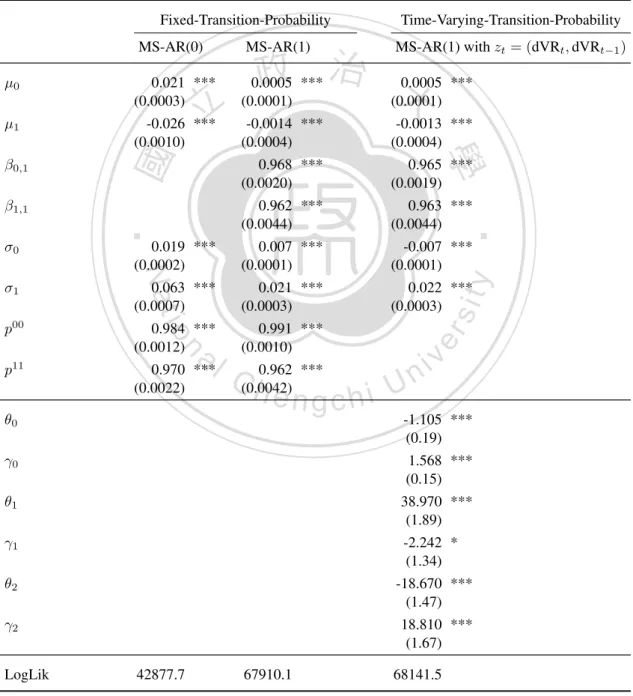
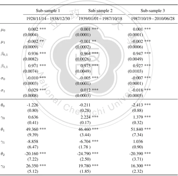
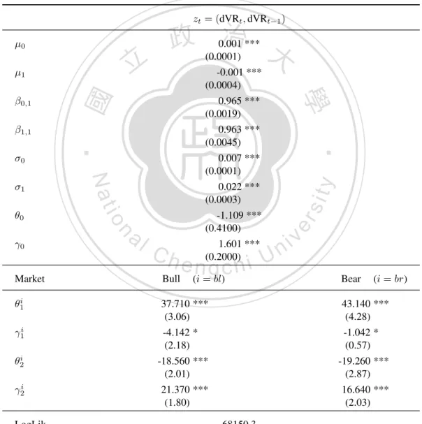
(4) In this chapter, we study how market volatility information affects trading signals generated from the technical analysis. Through the use of the time-varying-transition-probability (TVTP) Markov-switching model, we find that the increase of market volatility leads to a higher probability of signals generated from the VMA rule. Moreover, such an effect is asymmetric in bull and bear markets. This chapter also reexamines the value of market volatility in the simple MA rule by comparing the trading signals produced from the Fixed-transition-probability (FTP) and the TVTP Markov-switching model. Our results show that the time to enter or exit the market affected by market volatility information will benefit investors with higher profit.. 立. 政治大. ‧. ‧ 國. 學. n. er. io. sit. y. Nat. al. Ch. engchi. ii. i n U. v.

(5) Table of Contents 1. Introduction. 1. 2. Does Market Volatility Improve Profitability of Technical Analysis?. 3. 2.1. Introduction . . . . . . . . . . . . . . . . . . . . . . . . . . . . . . . . . . . .. 3. 2.2. Technical Trading Rules . . . . . . . . . . . . . . . . . . . . . . . . . . . . .. 6. 2.2.1. Static Trading Rules . . . . . . . . . . . . . . . . . . . . . . . . . . .. 6. 2.2.2. Dynamic Trading Rule . . . . . . . . . . . . . . . . . . . . . . . . . .. 7. 2.3. Methodology . . . . . . . . . . . . . . . . . . . . . . . . . . . . . . . . . . .. 10 10. 2.4. 治政大. . . . . . . . . . . . . . . Empirical Results on the Trading Rule Profitability 立 2.4.1 Data . . . . . . . . . . . . . . . . . . . . . . . . . . . . . . . . . . . . 學. 2.4.2. Data Snooping Bias and the SPA test . . . . . . . . . . . . . . . . . .. ‧ 國. 2.3.1. SPA Test Results: Full Sample and Sub-samples . . . . . . . . . . . .. Market Timing Ability Test. . . . . . . . . . . . . . . . . . . . . . . . . . . .. 2.6. Is the Profitability of the Trading Rule Asymmetric in Different Market Condi-. y. 24. er. al. Conclusion . . . . . . . . . . . . . . . . . . . . . . . . . . . . . . . . . . . .. n. 3. 18. 23. Market Timing Ability in Bull and Bear Market . . . . . . . . . . . . .. io. 2.7. 12. sit. Nat. tions? . . . . . . . . . . . . . . . . . . . . . . . . . . . . . . . . . . . . . . . 2.6.1. 12. ‧. 2.5. 12. Ch. engchi U. v ni. 31. Exploring the Information Content of Market Volatility in Technical Analysis. 32. 3.1. Introduction . . . . . . . . . . . . . . . . . . . . . . . . . . . . . . . . . . . .. 32. 3.2. Moving Average Trading Systems . . . . . . . . . . . . . . . . . . . . . . . .. 34. 3.2.1. Market Volatility in Moving Averages . . . . . . . . . . . . . . . . . .. 35. Trading Signals and Market Volatility Ratio . . . . . . . . . . . . . . . . . . .. 37. 3.3.1. The TVTP Markov-Switching Model . . . . . . . . . . . . . . . . . .. 38. 3.3.2. Data . . . . . . . . . . . . . . . . . . . . . . . . . . . . . . . . . . . .. 40. 3.3.3. Empirical Results . . . . . . . . . . . . . . . . . . . . . . . . . . . . .. 41. 3.3.4. Robustness . . . . . . . . . . . . . . . . . . . . . . . . . . . . . . . .. 45. 3.3. iii.

(6) 3.4.1. Data and Estimation Results . . . . . . . . . . . . . . . . . . . . . . .. 52. 3.4.2. The Profitability . . . . . . . . . . . . . . . . . . . . . . . . . . . . .. 56. 3.4.3. Simple Analysis for Trades . . . . . . . . . . . . . . . . . . . . . . . .. 58. The Future Way of Exploring Explanations for Higher Profits Gained from Market Volatility . . . . . . . . . . . . . . . . . . . . . . . . . . . . . . . . . . . .. 65. Conclusion . . . . . . . . . . . . . . . . . . . . . . . . . . . . . . . . . . . .. 68. 立. 政治大. 學 ‧ y. Nat. io. sit. 3.6. 51. n. al. er. 3.5. The Value of Market Volatility Ratio in Simple Moving Average Rule . . . . .. ‧ 國. 3.4. Ch. engchi. iv. i n U. v.

(7) List of Tables 1. Descriptive Statistics for Daily Changes in the Logarithm of DJIA index . . . .. 13. 2. The Performance of the Best Trading Rule in the Full Sample . . . . . . . . . .. 16. 3. The Performance of the Best Trading Rule in the Sub-Samples . . . . . . . . .. 17. 4. The Performance of the Best Trading Rule in Other Five Sub-Samples . . . . .. 18. 5. Cumby-Modest market timing tests for the best VMA, best MA and best MSV rule . . . . . . . . . . . . . . . . . . . . . . . . . . . . . . . . . . . . . . . .. 6. 22. Comparisons in the trading performances of the best VMA, best MA and best MSV rule . . . . . . . . . . . . . . . . . . . . . . . . . . . . . . . . . . . . .. 23. 7. Bull and bear markets in the DJIA daily price index . . . . . . . . . . . . . . .. 25. 8. Cumby-Modest market timing tests for the best VMA, best MA and best MSV. 立. 政治大. ‧ 國. 9. 學. rule in bull and bear markets . . . . . . . . . . . . . . . . . . . . . . . . . . . Comparisons in the trading performances of the trading rules in each market. ‧. condition . . . . . . . . . . . . . . . . . . . . . . . . . . . . . . . . . . . . . 10. 27. 29. Comparisons in the trading performances of one trading rule in different market. y. Nat. io. sit. conditions . . . . . . . . . . . . . . . . . . . . . . . . . . . . . . . . . . . . .. 30. Descriptive Statistics And Unit Root Tests . . . . . . . . . . . . . . . . . . . .. 12. Markov-Switching Models: Full Sample . . . . . . . . . . . . . . . . . . . . .. 13. Robustness Check: Sub-samples . . . . . . . . . . . . . . . . . . . . . . . . .. 48. 14. Robustness Check: Bull and Bear Markets . . . . . . . . . . . . . . . . . . . .. 49. 15. Descriptive Statistics And Unit Root Tests: dt From Six SMA Rules . . . . . .. 53. 16. The FTP Markov-Switching Models: The SMA Rules . . . . . . . . . . . . . .. 55. 17. The TVTP Markov-Switching Models: The SMA Rules . . . . . . . . . . . . .. 57. 18. Comparisons In Profitability Of Trades From The FTP and TVTP Markov-. n. al. er. 11. Ch. engchi. i n U. v. Switching Models . . . . . . . . . . . . . . . . . . . . . . . . . . . . . . . . . 19. 42 46. 59. The Number Of Four Types Of Trades From The FTP And TVTP MarkovSwitching Models . . . . . . . . . . . . . . . . . . . . . . . . . . . . . . . . .. v. 60.

(8) 20. Comparisons In The Performance Of Trades Between The FTP and TVTP Model: Similar Trades . . . . . . . . . . . . . . . . . . . . . . . . . . . . . .. 21. Comparisons In The Performance Of Trades Between The FTP and TVTP Model: Overlapping Trades . . . . . . . . . . . . . . . . . . . . . . . . . . . .. 63. Comparisons In The Performance Of Trades Between The FTP and TVTP Model: Different Trades . . . . . . . . . . . . . . . . . . . . . . . . . . . . .. 立. 政治大. 學 ‧. ‧ 國 io. sit. y. Nat. n. al. er. 22. 61. Ch. engchi. vi. i n U. v. 64.

(9) 1. Introduction. Technical analysis of financial markets involves forecasting asset prices and providing trading advices on the basis of visual examinations or certain quantitative summary measures of past price movements (Edwards and Magee, 1967; Murphy, 1986). In the literature, the technical analysis is primary based on the information of past prices and/or volumes. However, in addition to past prices and volumes, it is legitimate to question whether there exists other information that can improve the profitability of technical analysis. The study of Yamamoto (2012) shows the same thought by investigating technical rules that utilize information regarding the orderflow imbalance and order-book imbalances, although these information do not contribute to profiting in intraday trading.. 立. 政治大. LeBaron (1999) mentions that one possible factor that might drive predictability is volatility,. ‧ 國. 學. and high volatility periods might add extra risk to dynamic strategies implying a higher risk premium, and therefore greater predictability. In the study of Owen and Palmer (2012), they. ‧. found that the profits for a momentum trading strategy in the foreign exchange market exhibited a downward trend in nine countries, and this downward trend may be somewhat explained. y. Nat. io. sit. partly by the declining exchange rate volatility. The possible relationship between the volatility. n. al. er. and the profitability motivates us to think whether the volatility is an important information in. i n U. v. technical analysis, and whether the technical trading strategies that are formulated according to. Ch. engchi. such information can yield better profit? This thesis thus aims to investigate the profitability of the trading strategies based upon the information of market volatility. Compared to previous studies, this thesis makes a unique contribution to the body of knowledge on the value of the information of market volatility in the profitability of technical analysis. This thesis consists of two chapters. In the first chapter, we examine whether the information of market volatility can enhance the predictability of technical analysis on the Dow Jones Industrial Average (DJIA) index over 1928/10/1-2010/6/28, by the Superior Predictive Ability Test (SPA) proposed by Hansen (2005). We find strong evidence for the existence of statistically significant larger excess return to the technical trading rule formulated based upon the. 1.

(10) information of market volatility. Then we seeks to find evidence that can account for its better performance. Our results from the market timing test of Cumby and Modest (1987) clearly reveal that the technical trading rule with the information of market volatility enjoys better timings in generating profitable trading signals. Lastly, we further investigate whether the better predictive ability of the technical trading rule with market volatility is sensitive to different market conditions, We find that it outperforms other rules both in bull and bear markets, particular in bear markets. The second chapter seeks to explore how the market volatility ratio is informationally relevant for the determination of trading signals in technical analysis by the time-varying-transition-. 治政大of market volatility we adopt in technical trading rule formulated based on the information 立 this thesis is the Variable Moving Average (VMA), a variant of the Moving Average (MA) probability (TVTP) Markov-switching model. This is the second contribution in the thesis. The. ‧ 國. 學. system. Due to the specific trading mechanism in the MA system, the crossover, the nonlinear relationship between the market volatility and trading signals can be measured through the. ‧. TVTP Markov-switching model. Our estimation results demonstrate that the increase of market. sit. y. Nat. volatility leads to a higher probability of generating signals in technical analysis. Furthermore,. io. er. the effect is stronger in bear markets than in bull markets. While for a buying signal, its effect. al. in bull markets is larger than in bear markets. In the second chapter, we also seek to reex-. n. v i n amine the value of market volatilityCby the Fixed-transition-probability (FTP) and the TVTP hengchi U Markov-switching models for a particular Simple MA rule. This idea emerges from the trading rules (with and without market volatility) chosen to be compared in our previous study are based on different parameter settings and the time they generate signals are totally different. As a result, the worth of the information of market volatility in technical analysis can not be revealed directly. Through comparing the trading signals generated from the FTP and the TVTP Markov-switching models for a particular Simple MA rule, we can clearly see how the time the signal generated varies and how much more profit investors can get after the information of market volatility is considered in forecasting. Our results reveal that the time to enter or exit the market affected by market volatility information will benefit investors with higher profitability. 2.

(11) 2. Does Market Volatility Improve Profitability of Technical Analysis?. 2.1. Introduction. Technical analysis, based on the premise that price movement will repeat itself and then display regular or recurring pattern, is a method of forecasting future price movement relying only on the information of past prices and/or volumes. This method has a long history among investment professionals (Smidt, 1965; Allen and Taylor, 1992; Billingsley and Chance, 1996; Lui and Mole, 1998; Oberlechner, 2001; Gehrig and Menkhoff, 2004; Covel, 2005; Lo and Hasan-. 政治大 conflict with the central idea of the efficient market hypothesis. Thus, whether investors can get 立. hodzic, 2009). The essence of technical analysis and its widespread adoption by practitioners. ‧ 國. 學. statistically significant economic profits by technical analysis has drawn a lot of attention and discussion since Alexander (1961). Recent studies find more and more evidences of profitabil-. ‧. ity of technical analysis even by examining more trading systems or adopting stricter statistical tests solving data snooping bias problems (Brock et al., 1992; Chan et al., 1996; Neely et al.,. y. Nat. sit. 1997; Sullivan et al., 1999; LeBaron, 1999; Okunev and White, 2003; Hsu and Kuan, 2005;. n. al. er. io. Schulmeister, 2008). The consensus of these studies appears that using technical analysis helps investors to forecast the market.. Ch. engchi. i n U. v. In addition to technical analysis, market volatility investigation is also an important issue in the financial literature and there exists a lot of papers on modeling and estimating it. Furthermore, the market volatility is viewed as the valuable information and acts as a key input in numerous financial researches such as the portfolio diversifications, the hedging strategy investigations, and the asset pricing models. Many value-at-risk models also require the estimation of volatility parameter to measure the market risk. Despite the accumulating evidence on the value of technical analysis by examining different trading systems and the increasing importance of the market volatility as a key input in financial studies, little is known about the value of market volatility in technical analysis. What is the role of market volatility playing in technical analysis? Is it valuable for enhancing the profitability of technical analysis if it is used as an input in 3.

(12) the technical trading systems? In this paper we are interested in examining a number of related questions. First, we ask whether market volatility is useful in enhancing the profitability of the technical analysis in which market volatility acts as an important input in the technical trading systems. We adopt the variable moving average (VMA), a variant of the popular moving average system proposed first by Chande (1992). The VMA rule automatically adjusts its effective length of the moving average according to the changing market conditions measured by the level of market volatility. It is viewed as the representative of the technical analysis comprising the information of market volatility in this study. Market volatility in the VMA rule is built to detect whether the market. 治政大 strategy to detect the market words, market volatility here helps the moving average trading 立 trend more timely. We apply five most tested technical trading systems (filter, moving average, price makes big moves in up or down direction or whether it moves in a narrow range. In other. ‧ 國. 學. support and resistance, channel breakout, and momentum strategies in volume), and compare them with the VMA rule on the Dow Jones Industrial Average (DJIA) index over 1928/10/1-. ‧. 2010/6/28. In order to minimize data snooping bias, the Superior Predictive Ability Test (SPA). sit. y. Nat. proposed by Hansen (2005) is performed. Our SPA results both in full sample and several. io. al. significant greater profitability in the DJIA market.. er. subsample periods clearly demonstrate that the VMA rule outperforms others with statistically. n. v i n Since we find strong evidence forCthe existence of statistically significant larger excess return hengchi U. to the VMA rule, we then consider what the source of the larger excess returns of the VMA rule might be. That is we want to discuss the possible reason why market volatility betters the performance of the technical analysis. For any technical trading rule to be profitable, the stock return must be predictable. The higher predictability of stock returns permits the possibility of larger excess return of technical analysis. Therefore, we carry out the market timing tests described in Cumby and Modest (1987) to examine the comparative predictability of the best VMA rule. This test can be used for investigating the ability of a trading rule to predict the sign of the one-period-ahead excess return. In this study, we modify this test by regressing the excess return to three dummy variables, which represent three forecast positions of the rule, long, short 4.

(13) and no positions. By the modification, we can study the market timing ability of a trading rule in forecasting future price to rise or descend without losing the essence of the market timing tests. Since the VMA rule is the variant of the moving average system, we compare the market timing ability of the best VMA rule with that of the best MA rule. We also make comparisons between the market timing ability of the best VMA rule and that of the second best rule in our SPA results, which is the momentum strategies in volume (MSV) rule. There is strong evidence indicating that all of these three best rules can forecast the upward direction of future price movement well, but only the best VMA rule possesses predictive ability for future downward trends.. 治政大 In this study, different market trading rules is different due to different market conditions. 立 conditions are measured by bull and bear markets, which are identified with the dating algorithm Moreover, we are also interested in examining whether the market timing ability of the. ‧ 國. 學. of Pagan and Sossounov (2003). Our results show that the market timing ability of the best VMA, best MA and best MSV rule are all asymmetric in different market conditions. They are. ‧. good at detecting price rising trends in bull markets rather than in bear markets, while they do. sit. y. Nat. possess predictive ability of price decreases only for bear markets not for bull markets. Besides,. io. er. the best VMA rule gains higher daily profit and suffer less daily loss as it signals long (short). al. and short (long) positions in bull (bear) markets, respectively. As a whole, the best VMA rule. n. v i n C hrule both in bull and outperforms the best MA and best MSV bear markets. engchi U. The remainder of the paper is organized as follows: Section 2 outlines the technical trading. rules used in this study. The SPA test of Hansen (2005) is presented in Section 3. Section 4 contains the data description and the SPA results of full and several subsample periods. Section 5 provides evidence for the market timing ability of the best VMA, best MA and best MSV rule. Section 6 discusses whether these three best rules have differential performance in different market conditions, and Section 7 concludes the paper.. 5.

(14) 2.2. Technical Trading Rules. In this paper, technical analysis we adopt can be categorized into two groups, the first group is the technical analysis without the information of the market volatility, and the second one, in contrast, consolidates the market volatility to form the new moving average system. Each group of rules is explained below. 2.2.1. Static Trading Rules. For the first group, we consider five types of trading rules: filter, moving average, support and resistance (trading range break), channel breakout, and momentum strategies. These five types. 政治大 a lot of discussion in the literature. For the parameter values of each type of rules, we select a 立 of rules are very popular among the practitioners on financial markets and have already drawn. ‧ 國. and Wu (2006).. 學. fairly large variety that has been applied in Sullivan et al. (1999), Hsu and Kuan (2005), and Qi. ‧. Technical trading rules, even having different mechanisms or forms, are to identify a trend reversal at a relatively early stage and then ride on that trend until there exists evidence showing. y. Nat. sit. that the trend has reversed. A filter rule generates a buy (sell) signal when today’s closing price. er. io. rises (falls) by x % above (below) its most recent low (high). The moving average rule uses. al. n. v i n C h moving averageUmoves above (below) the m-period buy (sell) signal when the n-period shorter engchi n-period previous prices, including today’s price, to calculate an average value. It generates a. longer moving average. The support and resistance (trading range break) rule involves buying (selling) when the closing price rises above (falls below) the maximum (minimum) price over the previous n periods. The channel breakout rule is quite similar to the support and resistance rule. It uses the maximum and minimum price over the previous n periods to construct the channel with one limitation that is the difference between the maximum and minimum price should be within x. The channel breakout rule involves buying (selling) when the closing price moves above (below) the channel. The momentum strategy we adopt is the momentum strategy in volume. The momentum 6.

(15) strategy in volume has been widely analyzed in the literature. Momentum strategy’s signals are determined by the oscillator and the overbought/oversold level k. It generates a buy (sell) signal as the oscillator crosses the overbought (oversold) level from below (above). 2.2.2. Dynamic Trading Rule. VMA rule. In 1992, Chande proposed a variant of the moving average system, the VMA. rule. The main reason that Chande proposed this rule is that the existing technical trading rules are static and not responsive enough to the changing nature of markets. Static trading rules, by the definition, are the rules that do not change the length of the historical data used. 治政 means that market practitioners at each time use fixed n-length 大of the historical data to calculate 立 one moving average value, and then make trading decisions based on these calculations.. for forecast future price movement. For example, an n-length simple moving average strategy. ‧ 國. 學. The market is dynamically evolving with continuous changes; therefore, static trading rules with fixed length of data used in detecting the emergence of new trends may not work all the. ‧. time. For instance, consider two simple moving averages, a shorter moving average and a. sit. y. Nat. longer moving average. If the market is trending, making big moves in up or down direction,. io. er. the shorter moving average will response more quickly than the longer one since it gives more. al. weight to latest data and then may generate signal earlier. If the market, on the other hand, is. n. v i n ranging on which price trades in a narrow trend, the shorter moving average C h range without any engchi U will tend to produce numerous false trading signals due to its’ great proportion of more recent data, but the longer moving average desensitizes small erratic price movement and will generate fewer or no false signals. Due to the continuous changes in the market, Chande introduces a trading rule that can adapt itself to the market condition becoming a shorter moving average as the market is trending and automatically changing into a longer one when the market is ranging. He constructs the VMA rule by revising the exponential moving average as follows: EMAt = αPt + (1 − α)EMAt−1 ,. (1). 7.

(16) α=. 2 , N +1. (2). Here, EMAt is the exponential moving average value at time t, α is the numerical constant, N is the effective length of historical data used to calculate the exponential moving average value, Pt is the closing price at time t. Equation (1) is the traditional exponential moving average in which α is referred as the smoothing parameter describing the weight that the exponential moving average gives to the more recent data. As the smoothing parameter α increases (N decreases), the exponential moving average adopts less length of historical data and has a greater proportion of the latest data; therefore, it will trace the market price more closely. In contrast, as α decreases (N increases), more length of historical data is considered, greater weight is given. 政治大. to the more distant data and the gap between the exponential moving average and the current. 立. price will increase.. ‧ 國. 學. Since α is a constant and fixed term, it does not adjust to the changing nature of market in advance. Therefore, Chande improves the smoothing parameter of the exponential moving. ‧. average from constant to continuously variable by tying it to a market-related variable as below:. Nat. Ch. ,. (3). sit er. al. n. VRt =. σtn σtref. io. αt∗ = αVRt ,. y. VMAt = αt∗ Pt + (1 − αt∗ )VMAt−1 ,. engchi U. v ni. (4). (5). In Equation (3), VMAt is the variable moving average at time t, and the smoothing parameter here is αt∗ , which is variable, consists of the constant term α and the market variable VRt . VRt is the market volatility ratio viewed as a market variable and is formed by σtn and σtref . σtn is the standard deviation of closing prices over past n periods at time t, σtref is the reference standard deviation of closing prices over some period of time longer than n at time t.. The value of the market volatility. The most important part in the VMA rule is the market. volatility ratio, VRt . It is constructed in order to detect the market condition: the price action 8.

(17) is heating up or cooling down. It acts as the automatically adjusting device for choosing more suitable effective length of the historical data. The key idea of Chande’s VRt is that if the market is active with the trend, making big moves in up or down direction, the market price will change largely. Whether the market price changes largely or not might be measured by the standard deviation of closing prices, and a reference standard deviation is needed to tell us whether the observed standard deviation is too high or too low. Thus Chande attempts to use the ratio of σtn to σtref as the proxy of the market condition. The information of the market volatility makes the VMA a more responsive and smarter indicator than the exponential and the simple moving average. Consider the following three. 治政大 traders over the past n periods over the past n periods changes more largely than before because 立 adjust rapidly to new information. Since VR > 1, the VMA will take a larger bite of the new. situations. First, if σtn is greater than σtref , that is VRt > 1, it implies that the market price. t. ‧ 國. 學. data Pt and the effective length of the average decreases. Then the VMA will generate an earlier signal under the moving average crossover decision model. In the second situation in which σtn. ‧. is smaller than σtref (VRt < 1), market price over the past n periods moves in a narrow range. sit. y. Nat. due to no influential or new information on the market. When VRt < 1, the VMA takes a. io. er. smaller bite out of the new data, and the effective length of the average increases. Thus the. al. VMA will generate fewer false signals. In other words, the VMA will automatically become. n. v i n Cinto a shorter moving average or change one based on whether the market is active h ea nlonger i U h c g or not. Third, the VMA will become the exponential moving average when VR = 1 and the t. effective length of moving average will be determined only by the constant term, α.. The trading strategies in the VMA. For the trading strategies in the VMA, Chande mentions. that all the conventional strategies with the moving average system can be extended in the VMA. The most popular trading strategies is the moving average crossover decision model as follows: 1 1. For the parameter values of the VMA, the settings in Chande (1992) and Chande (1994) are adopted. We also consider the suggestions of some professional traders from the websites of professional trading companies.. 9.

(18) Buy when current price (shorter VMA) moves above the VMA (longer VMA). Sell when current price (shorter VMA) moves below the VMA (longer VMA).. 2.3 2.3.1. Methodology Data Snooping Bias and the SPA test. In the technical analysis literature, researchers typically can create a large number of trading rules by fine-tuning the parameters of the rules, and subsequently attempt to find a trading rule that yield the maximum excess return during the sample period. The major drawback of such an approach is that it often leads to the so-called data snooping bias. In other words, the. 政治大 sample period, and does not really 立 enjoy any predicting power of profitable opportunities (see most profitable trading rule so identified from historical data may only stand out in the selected. ‧ 國. 學. Lo and MacKinlay 1990.). In dealing with such data snooping bias, two major approaches are proposed in related. ‧. literature. First, to avoid data-mining the same data set repeatedly, Lakonishok et al. (1994), and Chan et al. (1998) suggest using different but comparable samples to examine profitability. y. Nat. sit. of trading rules. Such an approach may not work if no comparable samples are available. In. n. al. er. io. that case, Brock et al. (1992), Gencay (1998), and Rouwenhorst (1999) propose to test for. i n U. v. the profitability of trading rules not only for the entire long sample period, but also for many. Ch. engchi. sub-periods. Again, for adopting such an approach, one often needs to worry about how to split the long sample in an objective and convincing way. Second, to control for the test size, Lakonishok and Smidt (1988) apply the Bonferroni inequality in testing all possible models. Such an approach may present a practical difficulty in the case of technical analysis, as there exist too many trading rules to be considered. Along the same spirit of Lakonishok and Smidt (1988), White (2000) proposes the Reality Check (RC), which is capable of dealing with the data snooping bias, and handling a large number of trading rules at the same time. There are, however, two shortcomings of the RC: the average return in the RC are not standardized; and the RC fail to exclude trading rules that do not produce positive returns, which reduces the test. 10.

(19) power of the RC statistic. Consequently, Hansen (2005) proposed a more powerful Superior Predictive Ability (SPA) test with the following null hypothesis, H0SP A : µ ≤ 0, where. (6). µ = max {E(Rk )}, k=1,...,L. ¯ k = N −1 E(Rk ) = R. T X. ¯ k,t , k = 1, ..., L, R. t=p. k is the k th trading rule; L is the total number of trading rules; Rk denotes the return of the k th trading rule; T is the sample size; N ≡ T − p + 1 denotes total usable number of observations used in calculating the average returns; E(Rk ) is an L × 1 vector, and represents average returns. 政治大. of L different trading rules, with 0 denoting average return of the benchmark trading rule.. 立. Rejection of the null hypothesis represents that there exists at least one trading rule whose. ‧ 國. 學. average return is significantly greater than zero.. ‧. To implement the hypothesis testing, Hansen (2005) constructs the following test statistic √ ¯k ) N (R SP A , 0}, (7) TL = max { k=1,...,L ω bk. y. Nat. io. sit. where ω bk represents the standard error of trading rule k . Furthermore, Hansen (2005) propose. n. al. er. using the stationary bootstrap to come up with the empirical distribution of TLSP A √ N (ˆ µ∗c k,b,t ) SP A∗ TL,b = max { , 0}, b = 1, ..., B, k=1,...,L ω bk s ! 2 ω b ¯∗ ¯ ¯ √ k 2 log log N , where µ ˆ∗c k,b,t = Rk,b − Rk 1 Rk ≥ − N. Ch. engchi. i n U. v. (8). B is the total numbers of re-sampling; 1(·)is an indicator function, which is equal to 1 when the √ condition inside the indicator function is satisfied, and is equal to 0 otherwise; 2 log log N is the threshold rate. As long as the p-value of the test statistic is smaller than the significance level, we reject the null hypothesis, and hence there exists at least one trading rule with significantly positive average return.. 11.

(20) 2.4 2.4.1. Empirical Results on the Trading Rule Profitability Data. Data examined in this paper consists of the Dow Jones Industrial Average (DJIA) daily closing price from Oct 1, 1928 to June 28, 2010 - a collection of more than 80 years of daily data. In addition to the full sample, we also conduct sub-sample analysis as a robustness check. To create sub-samples, two criteria are adopted. First, we divide the full sample into two subsamples with equal lengths according to Qi and Wu (2006). Second, based on Brock et al. (1992), the full sample is split into the following five sub-samples: 1928/10/1−1938/12/31, 1939/1/1−1962/6/30, 1962/7/1−1986/12/31, 1987/1/1−1996/12/31, and 1997/1/1−2010/6/28.. 政治大. Table 1 reports some summary statistics for daily changes in the logarithm of DJIA index both. 立. for the full and sub-samples. We observe that the DJIA daily return distributions exhibit excess. ‧ 國. 學. kurtosis for the full and all sub-samples, and some of them are even strongly leptokurtic. The return of the k th technical trading rule at time t, Rk,t , is evaluated as follows:. (9). sit. y. Nat. k = 1, ..., L, t = 256, ..., T,. ‧. Rk,t = (lnPt − lnPt−1 ) · Ik,t−1 − |Ik,t−1 − Ik,t−2 | · g,. er. io. where Pt is the DJIA closing price at time t; It is a dummy variable, which is equal to 1 repre-. al. v i n g is the one-way transaction cost. C Here 0.05%, a round-trip transaction cost h ewensetg gcequal hi U n. senting a long position, 0 representing a neutral position, and -1 standing for a short position;. is therefore 0.1%; L describes the total number of the technical trading rule we apply in this. study, which is 5,162 in this study; t starts from 256 because some trading rules need 255 days of historical data to generate a trading signal, and T is the sample size, which is 20,526 for the full sample. 2.4.2. SPA Test Results: Full Sample and Sub-samples. In this subsection, we present the SPA test results on the profitability of 5,162 technical trading rules. Table 2 reports the performance of the best trading rule on each trading family in the full sample with the one-way transaction cost 0.05%. The first and second columns in Table 2 are 12.

(21) 13. 0.016 **. -0.026 ***. 0.014 ***. 0.012 ***. 0.005 ***. -0.024 ***. ρ(2). ρ(3). ρ(4). ρ(5). ρ(6). 27.707. Kurtosis. 14.273 -14.470 2.118 0.030 8.698 -0.027. 10.508 -25.632 1.085 -1.312. 39.862. er. -0.038 ***. 0.014 ***. 0.034 ***. -0.006 ***. -0.007 ***. -0.017 ***. 0.010 ***. -0.050s*** it. 0.017. -0.044. 0.013. 0.029. 0.016. 0.003. -0.017. 0.024. y. 2,558. Sub-sample 1. 10,263. v. 0.018. -0.008. 0.014. 19.817. -0.103. 1.239. -14.470. 14.273. 0.012. 10,263. engchi. ρ(1). -0.595. -25.632. Min. Skewness. 14.273. Max. 1.165. 0.018. Mean. Standard Deviation. 20,526. Sample Size. Sub-sample 2. Ch i n U. ‧. Sub-sample 1. Qi and Wu. n. Full. io. al. 學. Nat 5,888. Sub-sample 2. daily return. * denotes significance at the 10% level, ** denotes significance at the 5% level, and *** denotes significance at the 1% level.. ‧ 國. -0.028 ***. 0.018 ***. 0.049 ***. 0.015 ***. -0.056 ***. 0.118 ***. 13.873. -0.680. 0.783. -7.043. 9.090. 0.022. -0.020 ***. -0.012 ***. -0.003 ***. -0.003 ***. -0.001 ***. 0.145 ***. 5.273. 0.260. 0.842. -4.718. 4.952. 0.019. 6,157. Sub-sample 3. Brock et al.. -0.002 ***. 0.065 ***. -0.052 ***. -0.02 ***. -0.077 ***. 0.016. 142.523. -5.710. 1.066. -25.632. 9.666. 0.048. 2,529. Sub-sample 4. 0.005 ***. -0.038 ***. -0.003 ***. 0.042 ***. -0.063 ***. -0.067 ***. 10.039. -0.088. 1.276. -8.201. 10.508. 0.013. 3,394. Sub-sample 5. We have two types of sub-sample period. One is built according to Qi and Wu (2006), while another one is based on the criterion of Brock et al. (1992). Here ρ(k) is the kth order serial correlation of. This table reports summary statistics for daily return of DJIA index (in %) in the full and sub-sample periods. The full sample period is between Oct 1, 1928 and June 28, 2010, with 20,526 observations.. Table 1: Descriptive Statistics for Daily Changes in the Logarithm of DJIA index. 立. 政治大.

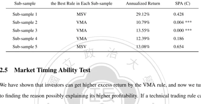
(22) the best rules on each trading family, and their rank in the universe of trading rules. The third, fourth, and fifth columns are their total number of trades, daily mean return and annualized return they obtain in this period. The last column reports the p−value of SPA test. We can observe that the overall best rule in the universe is the VMA family, and the best rule of the MSV wins the third place. The annual profits are 8.18%, 7.64%, 7.04%, 6.67%, 4.98%, and 2.64%, respectively, for the best rule of the VMA, MSV, MA, FR, CB, and the SR families. The best rule of the VMA, MSV, MA and FR families enjoy statistically significant profit at the 10% significant level, while profits from other two type of rules are all insignificant different from 0. To sum up the SPA test results for the full sample, as presented in Table 2 , we find. 政治大. that the VMA rule can earn statistically and economically significant profit, and it outperforms others with highest mean return.. 立. Table 3 describes the performance of the best rule on each trading family in the sub-samples.. ‧ 國. 學. Panel A and B demonstrate the results in the first and second sub-sample, respectively. Similarly, the best rule in the universe in these two sub-samples are all the VMA rules. It has eco-. ‧. nomically significant profitability due to its SPA p−value less than 5% in the first sub-sample.. sit. y. Nat. Except for the best rule of the VMA and MSV, other rules are insignificantly profitable in the. io. al. er. first sub-sample. And in the second sub-sample, the profitability of all types of rule is weaker.. n. We reject the null hypothesis for the performance of the best rule on the VMA family only at the 10% significant level.. Ch. engchi. i n U. v. Table 4 summarizes the performance of the technical trading rules in other five sub-samples. We just report the best one in the universe of 5,162 trading rules in each sub-sample with its annualized return and the SPA p−value. We can discover that three out of five best rules in these periods are the VMA rules (Sub-sample 2, 3, and 4), and the null hypothesis of the SPA test for Sub-sample 2 and 3 can be rejected even at 1% significant level. Although the best one in the Sub-sample 1 and 5 are the MSV rule, their profitability are all insignificant. To conclude the SPA results both for the full sample and all sub-samples, we can find that the performance of the VMA is more outstanding than other five rules. Besides, these results provide us the evidence that the information of market volatility does enhance the profitability 14.

(23) of the Moving Average system, as presented in Table 2 and Table 3. In the full and the two sub-samples, the best rules of the VMA are the entire best one in the universe of 5,162 trading rules, while the best rules of the MA in these periods merely win 7th, 13th, and 10th places in the universe, respectively.. 立. 政治大. ‧. ‧ 國. 學. n. er. io. sit. y. Nat. al. Ch. engchi. 15. i n U. v.

(24) 16 1878 410. 141. er. 988. best rule on the FR family: 0.05 filter rate、the highest and lowest price over the 2 most recent days.. best rule on the CB family: the high price over previous 5 days is within 0.01 of the low price over previous 5 days、0.0005 band、10 fixed holding days.. best rule on the SR family: the maximum(minimum) price over the previous 50 days by band 0.01、10 fixed holding days.. e The. f The. best rule on the MA family: 10-day short-run moving average、250-day long-run moving average、0.001 band.. c The. d The. best rule on the MSV (Momentum Strategy in Volume) family: 2-day moving average、250-day ROC、0.15 overbought/oversold rate、50 fixed holding days.. 2.64%. 4.98%. b The. 0.0105%. 0.0198%. 6.67%. 7.04%. 0.742. 0.492. 0.092 *. 0.050 *. 0.020 **. 0.006 ***. 8.18% 7.64%. SPA (C). Annualized Return. best rule on the VMA family: α = 0.049 (N = 40)、σt15,n 、σt30,ref 、0.0005 band.. y. 0.0265%. 23. 11. sit. 0.0279%. 49. 7. 3. v. a The. Note:. SR. 0.0303%. 400. engchi. f. CBe. FR. d. MAc. MSV. 0.0325%. 1. 563. Ch. b. VMAa. Daily Return. Number of Trades. i n U. ‧. Rank. al. Best Trading Rule in Each TA Family. 學. n. 252 trading days per annum. SPA (C) is the SPA p− value. * denotes significance at the 10% level, **denotes significance at the 5% level, and *** denotes significance at the 1% level.. io. return is computed from dividing the cumulative return in this period by the sample size (20,526 days). Annual return is calculated by multiplying the daily return by 252 because we have. Nat. their p-value on the SPA test. There are two signals, long and short, in one trade; therefore, the total trading number of the best VMA rule is 563 indicating that it has 1,126 signals. Daily. ‧ 國. trading rule in each trading family with their ranking in the universe of 5,162 rules, the number of trades, daily and annualized return they obtain with one-way transaction cost 0.05% , and. This table presents the SPA test results on the profitability of 5,162 technical trading rules for the period between Oct 1, 1928 and June 28, 2010. We report the performance of the best. Table 2: The Performance of the Best Trading Rule in the Full Sample. 立. 政治大.

(25) n. Rank. 17 583. 259. er. 1 2 4 10 25 1169. MSV. CB. MA. FR. SR. v. VMA. 156. 1105. 108. 391. 141. 306. 1775. 138. 0.0075%. 0.0237%. 0.0249%. 0.0268%. 0.0287%. 0.0310%. 0.0262%. 0.0294%. 0.0341%. 933. 13 39. y. 0.0515%. 0.0399%. sit. Daily Return. 583. 870. Number of Trades. 0.0430%. 4. i n U. Panel B: Sub-sample 2, 1969/10/29-2010/06/28. SR. FR. CB. MA. engchi. ‧. 198. Ch. MSV. 1. Panel A: Sub-sample 1, 1928/10/01-1969/10/28. al. VMA. io. Best Trading Rule in Each TA Family. ‧ 國. 學. Nat 1.89%. 5.97%. 6.28%. 6.75%. 7.23%. 7.82%. 6.61%. 7.40%. 8.60%. 10.06%. 1. 0.910. 0.848. 0.400. 0.170. 0.090 *. 0.848. 0.670. 0.400. 0.120. 0.077 *. 0.008 ***. 12.97% 10.83%. SPA (C). Annualized Return. respectively. * denotes significance at the 10% level, **denotes significance at the 5% level, and *** denotes significance at the 1% level.. Qi and Wu (2006). Panel A and B demonstrate the performance of the best trading rule in each trading family with one-way transaction cost 0.05% in the first and second sub-sample,. This table reports the SPA test results on the profitability of 5,162 technical trading rules in two sub-samples as a robustness check. The criterion used to create sub-samples is based on. Table 3: The Performance of the Best Trading Rule in the Sub-Samples. 立政治大.

(26) Table 4: The Performance of the Best Trading Rule in Other Five Sub-Samples This table reports the performance of the best one in the universe of 5,162 technical trading rules in each sub-sample. Five sub-samples are created by the measure taken in Brock et al. (1992). The annualized return of the best rule is calculated with one-way transaction cost 0.05%. SPA (C) is the SPA p− value. * denotes significance at the 10% level, **denotes significance at the 5% level, and *** denotes significance at the 1% level.. the Best Rule in Each Sub-sample. Annualized Return. Sub-sample 1. MSV. 29.12%. 0.428. Sub-sample 2. VMA. 10.79%. 0.004 ***. Sub-sample 3. VMA. 13.55%. 0.000 ***. Sub-sample 4. VMA. 12.39%. 0.186. Sub-sample 5. MSV. 13.08%. 0.654. 立. 政治大. SPA (C). Market Timing Ability Test. 學. ‧ 國. 2.5. Sub-sample. We have shown that investors can get higher excess return by the VMA rule, and now we turn. ‧. to finding the reason possibly explaining its higher profitability. If a technical trading rule can be profitable, the stock return must be predictable. Higher profitability of a trading rule might. y. Nat. sit. stem from that it possesses higher predictive ability for stock returns.. er. io. Tests of market timing ability are common ways to evaluate whether a forecast is to have. al. n. v i n C h newsletter recommendations managers, portfolio managers, investment or trading rules’ signals engchi U value or not in financial literature. These tests are regularly used to study whether mutual fund. offer any market timing ability (Henriksson, 1984; Cumby and Modest, 1987; Lee and Rahman, 1990; Graham and Harvey, 1996; Kho, 1996; Kleiman et al., 1996; Daniel et al., 1997; Neely and Weller, 1999; Bollen and Busse, 2001). For any trading rule, timing implies that excess returns are positive after its recommended long positions and negative after its recommended short positions. In other words, the forecasting ability of a trading rule can be evaluated by these tests. In this study, we apply the market timing ability tests by Cumby and Modest (1987) since it is often used for investigating whether a trading rule can predict the sign of a one-period-ahead. 18.

(27) excess return.2 This test is carried out by regressing excess returns on one forecast position measured by an indicator variable z, which is either + 1 or - 1, depending upon whether the trading rule signals a long or a short position. If a trading rule does possess forecasting ability, a significantly positive relation between the one-period-ahead excess return and the forecast position can be found. We extend the test of Cumby and Modest (1987) by studying forecasting ability of long positions and short positions separately and including the no-positions variable. By this extension, in addition to the market timing ability of long positions and short positions, we can also study the average direction of price changes when a trading rule recommends not to have any position.. 治政大MA rule. Besides, we also make forecasting ability of the best VMA rule with that of the best 立 comparisons between the market timing ability of the best VMA rule and that of the best MSV. Since the VMA rule is the variant of the Moving Average system, we focus on comparing the. ‧ 國. 學. rule, because the MSV rule is the second best in our previous SPA tests. In order to carry out a reliable hypothesis testing, in which the market timing ability of. ‧. the best VMA rule is compared with that of the best MA and best MSV rule, we apply the. sit. y. Nat. Seemingly Unrelated Regressions (SUR). We consider the specification of a system of three. io. al. n. as follows:. er. equations, each with three explanatory variables and 20,496 observations.3 The SUR model is. Ch. engchi. 4 log P = Xi βi + ei , i = VMA, MA, MSV,.   yVMA  y=  yMA  yMSV. . .   XVMA   , X =  X   MA   XMSV. . .   βVMA   , β =  β   MA   βMSV. 2. . i n U. v. .   eVMA   , e =  e   MA   eMSV. (10).    ,  . (11). The assumption that relative risk premiums are constant over the sample period is made in this study. Here we delete the first 30 observations since all of these three best rules need at least 30 days to generate trading signals. 3. 19.

(28) where. Xi = (z1i , z2i , z3i ),. z1i,t =. z2i,t =. z3i,t =.    1 if no position is held by the ith rule at time t,   0 otherwise.    1 if the short position is held by the ith rule at time t,   0 otherwise.    1 if the long position is held by the ith rule at time t,   0 otherwise. 0. βi = (β1i , β2i , β3i ) ,. 立. 政治大. ‧ 國. 學. For each i, 4 log P is 20,496 × 1, Xi is 20,496 × 3 and βi is 3 × 1. The dependent variable,. ‧. 4 log P , is the log return of the DJIA (multiplied by 100), and it can also be interpreted as the daily one-period-ahead excess return. The independent variables for each i are three forecast. y. Nat. sit. variables as follows, z1i,t , z2i,t and z3i,t . They are set to one when the ith rule recommends no. n. al. er. io. position, a short position, and a long position respectively; otherwise, they are zero. The sum. i n U. v. of these three dummy variables at time t is one. β1i , β2i and β3i are slope coefficients for the ith rule.. Ch. engchi. If the ith rule does possess ability to detect future downward and upward trends, β2i and β3i will be significantly negative and positive, respectively. A positive β2i (negative β3i ) denotes that the ith rule predicts there will be a downward (upward) trend in the future, but the actual price rises (falls). Further, we can interpret the value of β2i (β3i ) as the mean profit/loss per day over the period in which the ith rule signals short (long) positions. Then β1i can be explained as the mean price change as the ith rule recommends not to have any position. In Panel A of Table 5, we present the estimation results for the SUR model along with the Newey-West (1987) robust standard errors. First of all, there is strong evidence indicating that the best VMA rule does have predictive ability for both upward and downward price movements, while the 20.

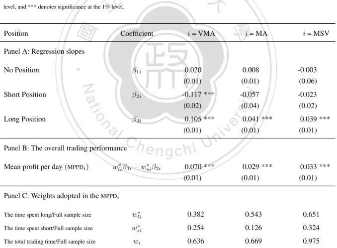
(29) best MA and best MSV rule are only capable of detecting upward price movements. We also compare the mean profit per day based on signals of long position and short-position issued by the best VMA rule, the best VMA rule, and the best MSV rule. The Wald test results in Table 6 show that the mean profit the best VMA rule gains from its long positions is significantly greater than those of the others. Its mean profit over the short-position periods is significantly greater than that of the best MSV rule, while there is no significant difference in the average short-position profit between the best VMA rule and the best MA rule. In addition to mean profits over the short-position periods and the long-position periods for the three competing rules (based on the size and value of β2 and β3 ), we also compute the mean profit per day (MPPD) as follows:. 立. ∗ ∗ MPPDi = wli β3i − wsi β2i ,. 政治大. (12). ‧ 國. 學. ∗ for each rule are the proportion of time spent on long positions and on where wli∗ and wsi. short positions relative to the entire sample period, respectively. Essentially, the MPPD can. ‧. be interpreted as an overall performance measure of a trading rule, which is weighted by the. sit. y. Nat. proportions of time spent on long positions and short positions. The results are reported in. io. er. Panel B and C of Table 5. All of those three rules have significantly positive mean profit per. al. day. Furthermore, the best VMA rule earns more than the others, as presented in Table 6.. n. v i n To summarize, the fact that theC best VMA can predict both upward and downward price hengchi U. movements, while other competing rules are only capable of detecting upward price movement give a strong evidence that higher profitability of the VMA rule might just stems from its better forecasting ability of stock returns. In addition, the results that the time the best VMA spent in the market is the least (roughly 63.6%), while the mean profit it gains in the market is the most (see Table 6), offer another piece of evidence that the best VMA rule does enjoy a better timing in generating profitable trading signals.. 21.

(30) Table 5: Cumby-Modest market timing tests for the best VMA, best MA and best MSV rule We carry out Cumby-Modest market timing tests by applying Seemingly Unrelated Regressions (SUR) as follows: 4 log P = Xi βi + ei , i = VMA, MA, MSV, where Xi = (z1i , z2i , z3i ) and βi = (β1i , β2i , β3i )0 . For each equation i, the dependent variable 4 log P , is the log return of the DJIA (multiplied by 100). The independent variables, z1i,t , z2i,t and z3i,t , are three dummy variables. They are set to one when the ith rule recommends no position, a short position, and a long position respectively; otherwise, they are set to zero. β1i , β2i and β3i are slope coefficients for the ith rule. We use wl∗ and ws∗ , the proportion of the time spent long and short to the full sample period, to measure a trading rule’s overall performance, the mean profit per day (MPPD). Panel A reports the regression results for the best VMA, best MA. 政治大. and best MSV rule, respectively. Panel B presents their overall performances. The wl∗ and ws∗ of each rule is reported in Panel C. In the parentheses are the Newey-West (1987) robust standard errors. * denotes significance at the 10% level, ** denotes significance at the 5%. 立. 學. Position. ‧ 國. level, and *** denotes significance at the 1% level.. i = VMA. Coefficient. i = MA. i = MSV. Panel A: Regression slopes. 0.020 (0.01). β2i. -0.117 *** (0.02). β3i. 0.105 *** (0.01). n. al. β1i. Ch. Panel B: The overall trading performance Mean profit per day (MPPDi ). engchi. ∗ ∗ wli β3i − wsi β2i. y. 0.008 (0.01). sit. -0.057 (0.04). er. io. Long Position. Nat. Short Position. ‧. No Position. i n U. 0.070 *** (0.01). v. -0.003 (0.06) -0.023 (0.02). 0.041 *** (0.01). 0.039 *** (0.01). 0.029 *** (0.01). 0.033 *** (0.01). Panel C: Weights adopted in the MPPDi The time spent long/Full sample size. ∗ wli. 0.382. 0.543. 0.651. The time spent short/Full sample size. ∗ wsi. 0.254. 0.126. 0.324. The total trading time/Full sample size. wi. 0.636. 0.669. 0.975. 22.

(31) Table 6: Comparisons in the trading performances of the best VMA, best MA and best MSV rule This table reports comparisons between the trading performances of the best VMA rule and that of the best MA and best MSV rule. For the ith rule, the value of β2i and β3i can be interpreted as the mean profit/loss per day over its short-position periods and long-position periods, while β1i is the average excess return when there is no signal released by this rule. The MPPDi measures its mean profit per day. These comparisons are implemented by the Wald test based on the Newey-West (1987) covariance matrix. In the parentheses are the Newey-West (1987) robust standard errors. * denotes significance at the 10% level, ** denotes significance at the 5% level, and *** denotes significance at the 1% level.. Position. Comparison. No Position. β1i − β1j = 0. Short Position. β2i − β2j = 0. Long Position. β3i − β3j = 0. 政治大. Overall Performance. 0.023 (0.06). -0.060 (0.04). -0.093 *** (0.03). 0.064 *** (0.01). 0.066 *** (0.01). 0.040 *** (0.01). 0.037 *** (0.01). ‧. Is the Profitability of the Trading Rule Asymmetric in Different Mar-. sit. y. Nat. 2.6. ∗ ∗ ∗ ∗ β3i − wsi β2i ) − (wlj β3j − wsj β2j ) (wli MPPDi − MPPDj. i = VMA, j = MSV. 0.012 (0.02). 學. ‧ 國. 立. i = VMA, j = MA. io. n. al. er. ket Conditions?. i n U. v. In the previous section, we have demonstrated a close connection between the VMA rule’s. Ch. engchi. higher profitability and its better forecasting ability for stock returns. This entails two interesting questions. First, is the predictive ability of the VMA rule for future price movements sensitive to different market conditions? Second, if so, does the VMA rule still enjoy higher profitability in all market conditions? To describe the evolution of the market condition, cyclical variations in stock returns have been widely reported (Turner et al., 1989; Hamilton and Lin, 1996; Perez-Quiros and Timmermann, 2000; Perez-Quiros and Timmermann, 2001.) Typically, bull markets and bear markets are commonly adopted to characterize equity cycles (Fabozzi and Francis, 1979; Hardouvelis and Theodossiou, 2002; Guidolin and Timmermann, 2005; Chen, 2007; Jansen and Tsai, 2010.) As a stylized fact, bull markets are usually associated with higher average stock returns, and a 23.

(32) lower variance; while bear markets are associated with lower average, but a more volatile stock returns. Specifically, we are interested in investigating whether the profitability of the VMA rule in bull markets is significantly different from that in bear markets? If the profitability of the VMA rule in bear markets is significantly higher, it may imply that the information of market volatility in bear markets is more crucial for technical trading rules to forecast future price movements. In this study, the dating algorithm proposed by Pagan and Sossounov (2003) is used to identify bull markets and bear markets in the DJIA daily index.4,5 According to Pagan and Sossounov (2003), a bull market occurs during the period when the stock price rises from a. 治政 price moves from a peak point to a trough point. With this 大 dating algorithm, all possible peaks 立 and troughs in the DJIA index can be found and subsequently be used to identify bull markets trough point and ends in a peak point; while a bear market exists during the period as the stock. ‧ 國. 學. and bear markets. Table 7 presents a summary of all bull markets and bear markets so identified. There are 23 and 22 mutually exclusive and exhaustive bull markets and bear markets. We can. ‧. find that, on average, durations of bull markets tend to be longer than those of bear markets in. sit. y. Nat. the DJIA. Specifically, Bull markets have lasted for an average of 28 months (583 days), while. io. er. bear markets have lasted for 15 months (324 days). Table 7 also shows that bull markets are. al. associated with higher but more stable stock returns while bear markets are associated with low. n. v i n C hare coincident withUthe findings in the literature. but volatile stock returns. These results engchi 2.6.1. Market Timing Ability in Bull and Bear Market. To ascertain whether the VMA rule has asymmetric, yet still dominating, performance over the equity cycles, the test of Cumby and Modest (1987) introduced in Section 2.5 is applied here again with the number of independent variables for each rule Xi extended from three to six as 4. The dating algorithm of Pagan and Sossounov (2003) is presented in the Appendix. The original parameter settings in Pagan and Sossounov’s dating algorithm are suitable for monthly data. In order to apply this algorithm to daily data, we revise the parameters based on the premise that there is 21 trading days in one month. 5. 24.

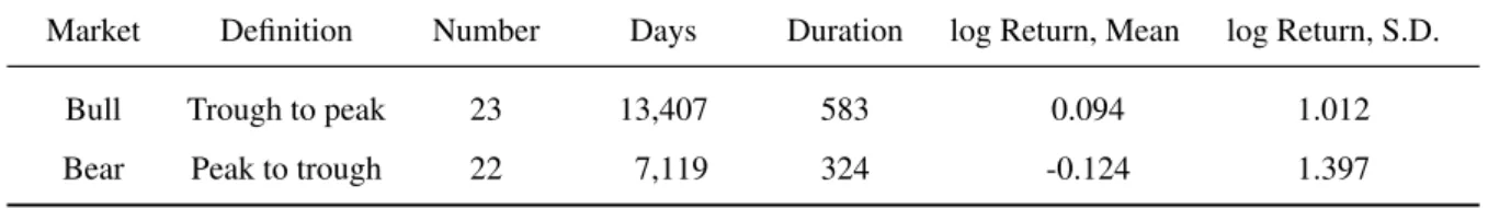
(33) Table 7: Bull and bear markets in the DJIA daily price index This table reports a summary of the bull and bear markets identified with Pagan and Sossounov (2003) algorithm over the full sample period. In the ”Days” and ”Duration” columns, we record the number of days for the whole bull and bear markets and the average days a bull or a bear market lasts.. Market. Definition. Number. Days. Duration. log Return, Mean. log Return, S.D.. Bull. Trough to peak. 23. 13,407. 583. 0.094. 1.012. Bear. Peak to trough. 22. 7,119. 324. -0.124. 1.397. follows:. 政治大. (13). bl bl bl br br br Xi = (z1i , z2i , z3i , z1i , z2i , z3i ), i = VMA, MA, MSV,. 立. bl bl bl are and z3i , z2i where the superscript bl and br represent bull and bear markets in the DJIA; z1i. ‧ 國. 學. dummy variables of the ith rule in bull markets, which are set to one when the ith rule in bull markets recommends no position, a short position, and a long position respectively; otherwise,. ‧. br br br are the corresponding dummy variables for the and z3i , z2i they are set to zero; similarly, z1i. sit. y. Nat. bl bl bl br br br ith rule in bear markets. Correspondingly, β1i , β2i , β3i , β1i , β2i and β3i are the associated slope. io. er. coefficients for the ith rule. If the ith rule can forecast future price increases (decreases) in all. al. br bl br bl ) should be significantly positive (negative). We also and β2i (β2i and β3i market conditions, β3i. n. v i n C hperformance of theUrule. use MPPD to measure the overall trading engchi. Table 8 reports the results of Cumby-Modest market timing tests for the best VMA, best MA. and best MSV rule in bull markets and bear markets. According to the estimated results, the predictive ability of the best VMA rule for price movements is indeed asymmetric in bull and bear markets. It can forecast price increases in bull markets, but not in bear markets. Conversely, it is capable of detecting downward price actions in bear markets but not in bull markets. For the best MA and the best MSV rule, the asymmetry in their respective forecasting ability under different market conditions still exists, and is similar to that in the best VMA rule. Moreover, they incur losses significantly on average as they forecast price increases in bear markets and price decreases in bull markets. 25.

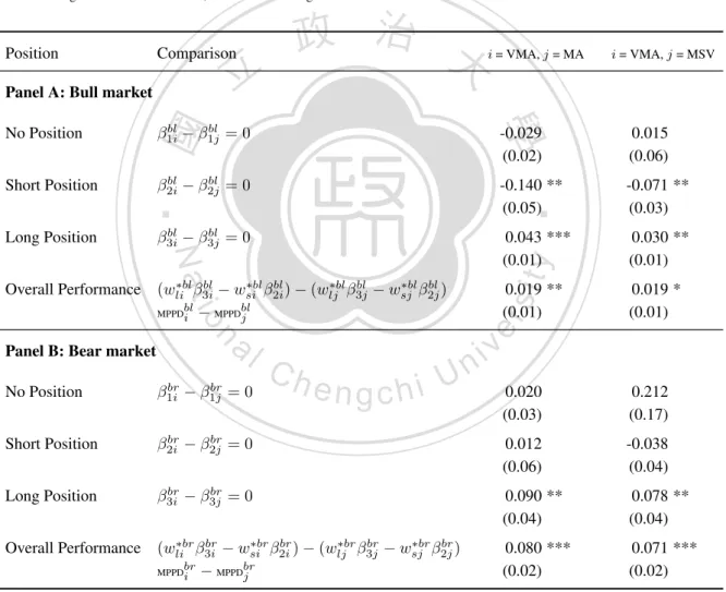
(34) As reported in Table 9, the profitability, measured by the MPPD, of the best VMA rule in bull and bear markets are all significantly higher than those of the best MA and the best MSV rule. This answers our second question. In other words, the higher profitability of the best VMA rule is not sensitive to different market conditions. In bull markets, the mean profit from the long positions signaled by the best VMA rule is significantly higher, and the mean loss entailed from its short-position signals is significantly less than the other two trading rules. In bear markets, although there is no significant difference between the mean profit in the downward forecasting of the best VMA rule and those of the others, the best VMA rule has significant less mean loss in the upward prediction.. 治政大 profit of the best VMA rule is MSV rule are not significantly different from 0, while the mean 立 significantly positive. as shown in Panel B of Table 8. This offers another piece of evidence that, It is noteworthy that, in bear markets, the mean profit of the best MA rule and the best. ‧ 國. 學. when asset prices change rapidly or drastically on the market, technical trading rules which do not incorporate any market volatility information cannot respond enough to the changing market. ‧. conditions. Therefore, our results suggest the information of market volatility in this kind of. sit. y. Nat. market should be seriously considered in technical trading rules. Another interesting result in. io. er. Table 10 is that the trading performance of the best VMA rule in bear markets is better than that. al. in bull markets. As mentioned before, better profitability of the VMA rule in bear markets may. n. v i n C h movements, the market imply that the device for detecting price volatility ratio, is particularly engchi U suitable for bear markets.. 26.

(35) Table 8: Cumby-Modest market timing tests for the best VMA, best MA and best MSV rule in bull and bear markets The market timing test for the trading rules in bull and bear markets is carried out by Seemingly Unrelated Regressions (SUR) as follows: 4 log P = Xi βi + ei , i = VMA, MA, MSV, bl , z bl , z bl , z br , z br , z br ) and β = (β bl , β bl , β bl , β br , β br , β br )0 . For each equation i, the dependent variable, where Xi = (z1i i 2i 3i 1i 2i 3i 1i 2i 3i 1i 2i 3i. 4 log P , is the log return of the DJIA (multiplied by 100). The market conditions, bull and bear markets, are represented by the index bl bl , z bl and z bl , (z br , z br and z br ), are dummy variables for bull (bear) markets. They are and br. The independent variables, z1i,t 2i,t 3i,t 1i,t 2i,t 3i,t. set to one when the ith rule in bull (bear) markets recommends no position, a short position, and a long position respectively; otherwise, bl , β bl and β bl (β br , β br and β br ) are the associated slope coefficients for the ith rule in bull markets. Panel A they are set to zero. β1i 2i 3i 1i 2i 3i. reports the regression results and trading performances for these three best rules in bull markets while the corresponding results in bear markets are presented in Panel B. We use wl∗ and ws∗ to measure the trading performance of the rule, the mean profit per day (MPPD).. 政治大. wl∗bl (ws∗bl ) is defined as the proportion of the time spent long (short) to all bull periods, while wl∗br (ws∗br ) is the ratio the trading rule spent for long (short) positions to all bear periods. The results are reported in Panel C on next page. In the parentheses are Newey-West. 立. (1987) robust standard errors. * denotes significance at the 10% level, ** denotes significance at the 5% level, and *** denotes significance. i = VMA. Coefficient. 學. Position. ‧ 國. at the 1% level.. i = MA. i = MSV. Panel A: Bull markets. 0.026 (0.03). al β. n. bl 3i. Long Position Overall Performance. ∗bl bl ∗bl bl β3i − wsi β2i wli bl (MPPDi ). Ch. y. bl β2i. 0.105 *** (0.02). sit. io. 0.077 *** (0.01). 0.062 (0.06). 0.166 *** (0.05). 0.098 *** (0.02). 0.080 *** (0.01). 0.093 *** (0.01). (0.01). 0.040 *** (0.01). 0.041 *** (0.01). 0.123 *** (0.01). U i *** e n g c h0.059. er. Nat. Short Position. bl β1i. ‧. No Position. v ni. Panel B: Bear markets No Position. br β1i. -0.078 *** (0.02). -0.098 *** (0.02). -0.289 * (0.17). Short Position. br β2i. -0.195 *** (0.03). -0.207 *** (0.05). -0.157 *** (0.03). Long Position. br β3i. -0.016 (0.03). -0.107 *** (0.02). -0.094 *** (0.02). 0.090 *** (0.01). 0.010 (0.01). 0.019 (0.02). Overall Performance. ∗br br ∗br br wli β3i − wsi β2i br (MPPDi ). 27.

(36) Table 8 Continued Measurement. i = VMA. Weight. i = MA. i = MSV. Panel C: Weights adopted in measuring a technical trading rule’s performance Bull market The time spent long/All bull periods. ∗bl wli. 0.511. 0.658. 0.709. The time spent short/All bull periods. ∗bl wsi. 0.138. 0.077. 0.261. The total trading time/All bull periods. wibl. 0.649. 0.735. 0.970. The time spent long/All bear periods. ∗br wli. 0.141. 0.327. 0.544. The time spent short/All bear periods. ∗br wsi. 0.473. 0.217. 0.443. wibr. 0.614. 0.544. 0.987. Bear market. The total trading time/All bear periods. 立. 政治大. ‧. ‧ 國. 學. n. er. io. sit. y. Nat. al. Ch. engchi. 28. i n U. v.

(37) Table 9: Comparisons in the trading performances of the trading rules in each market condition This table reports comparisons between the trading performances of the best VMA rule and that of the best MA and best MSV rule in bull bl and β bl and bear markets, respectively. Bull and bear markets are represented by the index bl and br. For the ith rule, the value of β2i 3i br and β br ) can be interpreted as the mean profit/loss over its short-position periods and long-position periods in bull (bear) markets, (β2i 3i bl (β br ) is the average excess return over the no-position periods in bull (bear) markets. while β1i 1i. profit per day the. ith. br MPPDbl i (MPPDi ). measures the mean. rule gains in bull (bear) markets. These comparisons are implemented by the Wald test based on the Newey-West. (1987) covariance matrix. The Newey-West (1987) robust standard errors are in the parentheses. * denotes significance at the 10% level, ** denotes significance at the 5% level, and *** denotes significance at the 1% level.. Position. Comparison. 立. Long Position. bl bl β1i − β1j =0. 0.015 (0.06). bl bl β2i − β2j =0. -0.140 ** (0.05). -0.071 ** (0.03). bl bl β3i − β3j =0. 0.043 *** (0.01). 0.030 ** (0.01). n. No Position. br br β1i − β1j =0. Short Position Long Position. Ch. engchi. 0.019 ** (0.01). er. io. al. sit. y. Nat. ∗bl bl ∗bl bl ∗bl bl ∗bl bl Overall Performance (wli β3i − wsi β2i ) − (wlj β3j − wsj β2j ) bl bl MPPDi − MPPDj. Panel B: Bear market. i = VMA, j = MSV. -0.029 (0.02). ‧. Short Position. 學. No Position. i = VMA, j = MA. ‧ 國. Panel A: Bull market. 政治大. i n U. 0.019 * (0.01). v. 0.020 (0.03). 0.212 (0.17). br br β2i − β2j =0. 0.012 (0.06). -0.038 (0.04). br br β3i − β3j =0. 0.090 ** (0.04). 0.078 ** (0.04). 0.080 *** (0.02). 0.071 *** (0.02). ∗br br ∗br br ∗br br ∗br br Overall Performance (wli β3i − wsi β2i ) − (wlj β3j − wsj β2j ) br br MPPDi − MPPDj. 29.

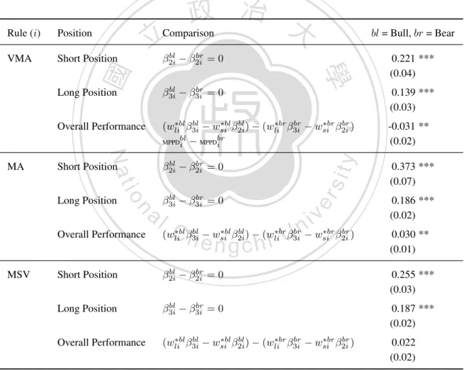
(38) Table 10: Comparisons in the trading performances of one trading rule in different market conditions This table reports comparisons between the trading performances of one trading rule, including the best VMA, best MA, and best MSV rule, in bull markets and that in bear markets. Bull and bear markets are represented by the index bl and br respectively. For the ith rule, bl and β br (β bl and β br ) can be explained as the mean profit/loss over its short-position (long-positions) periods in bull and the value of β2i 2i 3i 3i br bear markets, while MPPDbl i and MPPDi measure its mean profit per day in these two market conditions. We use the Wald test to implement. these comparisons, based on the Newey-West (1987) covariance matrix. In the parentheses are the Newey-West (1987) robust standard errors. * denotes significance at the 10% level, ** denotes significance at the 5% level, and *** denotes significance at the 1% level.. Position. VMA. Short Position. 立. bl br β2i − β2i =0. Overall Performance. ∗bl bl ∗bl bl ∗br br ∗br br (wli β3i − wsi β2i ) − (wli β3i − wsi β2i ) bl br MPPDi − MPPDi. y. ‧. bl br β3i − β3i =0. n. er. io. al. sit. bl br β2i − β2i =0. Short Position Long Position. bl br β3i − β3i =0. Ch. n U engchi. iv. 0.221 *** (0.04) 0.139 *** (0.03) -0.031 ** (0.02) 0.373 *** (0.07) 0.186 *** (0.02). ∗bl bl ∗bl bl ∗br br ∗br br (wli β3i − wsi β2i ) − (wli β3i − wsi β2i ). 0.030 ** (0.01). Short Position. bl br β2i − β2i =0. 0.255 *** (0.03). Long Position. bl br β3i − β3i =0. 0.187 *** (0.02). Overall Performance. ∗bl bl ∗bl bl ∗br br ∗br br (wli β3i − wsi β2i ) − (wli β3i − wsi β2i ). 0.022 (0.02). Overall Performance. MSV. 學. Long Position. Nat. MA. bl = Bull, br = Bear. Comparison. ‧ 國. Rule (i). 政治大. 30.

(39) 2.7. Conclusion. In this paper, we examine whether the information of market volatility is able to improve the profitability of technical analysis. In the previous literature, market volatility acts as a key input in many financial issues. It is, however, not clear whether market volatility has any value in technical analysis. That is, could the information of market volatility enhance the profitability of technical trading rules? If it does, why and how does it work? We adopt the VMA rule proposed by Chande (1992) as the representative of technical analysis comprising the information of market volatility. Market volatility in the VMA rule is built to detect whether the market price makes big moves in up or down direction or whether it moves. 政治大 trend timelier, the VMA rule should be more profitable than other rules. 立. in a narrow range. If the market volatility does help the technical trading rules to detect market. ‧ 國. 學. Using the Superior Predictive Ability test proposed by Hansen (2005), we find that the VMA rule outperforms others with higher profitability. Then we carry out the market timing ability. ‧. test of Cumby and Modest (1987), and compare the predictive ability for upward and downward trends of the best VMA rule with that of the best MA and best MSV rule. The results that the. y. Nat. al. er. io. of market volatility in better trend detecting ability.. sit. best VMA rule enjoys better market timing ability may provide evidence to support the value. n. v i n C h results suggest Uthat in bull markets, the best VMA, Empirical engchi. Finally, we also investigate whether the best VMA rule has differential market timing ability in different market conditions.. best MA and best MSV rule do possess predictive ability for future upward trends, but the best VMA rule earns more daily profit than the others. On the other hand, the average loss per day the best VMA rule suffers is less than that of the best MA and best MSV rule in downward trend forecasts. In bear markets, the best VMA rule as well as the best MA and best MSV rule is able to forecast a price decrease well; however, the best VMA rule has less daily loss than the others in the upward trend forecast. As a whole, the best VMA rule outperforms the best MA and best MSV rule both in bull and bear markets.. 31.