位元平面之壓縮取樣搭配貝氏估計解碼法於失真壓縮之應用

國

立

交

通

大

學

電子工程學系 電子研究所碩士班

碩

士

論

文

位元平面之壓縮取樣搭配貝氏估計解碼法

於失真壓縮之應用

Bit-plane Compressive Sensing with Bayesian Decoding

for Lossy Compression

研 究 生： 吳思賢

指導教授： 蔣迪豪 教授

彭文孝 教授

位元平面之壓縮取樣

搭配貝氏估計解碼法於失真壓縮之應用

Bit-plane Compressive Sensing

with Bayesian Decoding for Lossy Compression

研 究 生： 吳思賢

Student：

Sz-Hsien Wu

指導教授： 蔣迪豪

Advisor：

Tihao Chiang

彭文孝

Wen-Hsiao Peng

國 立 交 通 大 學

電子工程學系 電子研究所碩士班

碩 士 論 文

A Thesis

Submitted to Department of Electronics Engineering & Institute of Electronics College of Electrical and Computer Engineering

National Chiao Tung University in partial Fulfillment of the Requirements

for the Degree of Master of Science

in

Electronics Engineering July 2010

Hsinchu, Taiwan, Republic of China

i

位元平面之壓縮取樣搭配

貝氏估計解碼法於失真壓縮之應用

學生：吳思賢

指導教授：蔣迪豪

彭文孝

國立交通大學 電子工程學系 電子研究所碩士班

摘

要

本論文探討的問題是：當壓縮取樣點已遭受失真破壞，甚至取樣點亦嚴重不足的情 況下，如何能夠有效地重建回原本的稀疏訊號。而這樣的過程涉及如何估計稀疏訊 號子空間和稀疏訊號非零係數，在本研究中，我們依據最大後驗機率估計理論 (MAP)，推導了一組向量化的估計函數。藉著充分利用訊號的前驗機率，使得我們 提出的作法，可以利用極少、接近稀疏訊號非零係數個數的取樣點，即可進行完美 重建！同時，在取樣點嚴重不足的情況下預測稀疏訊號子空間時，本方法亦比前人 方法有更低的錯誤預測機率。此外，為了能更佳地重建稀疏訊號的重要資訊，我們 提出了位元平面切割方法。當這樣的技術與 MAP 估計函數相結合後，我們實證其可 得到與泛用 JPEG 標準相匹敵的壓縮性能：在同樣的壓縮品質下，其壓縮率差距小 於一倍。除此之外，我們亦將這個嶄新的技術應用於多重描述編碼，結果亦顯示我 們設計的 MAP 估計方法，即使是在流失率極嚴重的摧毀式通道環境，還是能夠提供 明顯良好的解碼品質。總而言之，相較前人研究成果，我們的壓縮取樣系統搭配 MAP 貝氏估計解碼法，不僅能提供極佳的壓縮性能，同時亦保有極為強悍的錯誤扺 抗能力。

ii

Bit-plane Compressive Sensing with

Bayesian Decoding for Lossy Compression

Student： Sz-Hsien Wu

Advisors： Dr. Tihao Chiang

Dr. Wen-Hsiao Peng

Department of Electronics Engineering & Institute of Electronics

National Chiao Tung University

ABSTRACT

This thesis addresses the problem of reconstructing a compressively sampled

sparse signal from its lossy and possibly insufficient measurements. The

process involves estimations of sparsity pattern and sparse representation, for

which we derived a vector estimator based on the Maximum a Posteriori

Probability (MAP) rule. By making full use of signal prior knowledge, our

scheme can use a measurement number close to sparsity to achieve perfect

reconstruction. It also shows a much lower error probability of sparsity

pattern than prior work, given insufficient measurements. To better recover

the most significant part of the sparse representation, we further introduce the

notion of bit-plane separation. When applied to image compression, the

technique in combination with our MAP estimator shows promising results as

compared to JPEG: the difference in compression ratio is seen to be within a

factor of two, given the same decoded quality. More than this, we also

applied such framework into the application of multiple description coding.

According to the simulation results, our MAP estimator is very resilient to the

loss of measurements, showing an acceptable quality while coping with a

highly loss channel. In conclusion, our CS framework using the MAP

estimation can provide a much better compression efficiency and stronger

functionality of error-resilience, compared with other prior work.

誌

謝

做研究，真的是一份不簡單的工作！雖然在大四升碩一的暑假，彭文孝老師就 決定讓我研究這個充滿數學挑戰的訊號處理新技術：Compressive Sensing。但我 絕對沒有想到，這個研究還是要耗時我近兩年的時間，才得以完成一個階段。在過 去兩年中，從數學理論到實驗證明，彭老師常強迫我自行獨立思考和解決問題，而 不直接給予明確的解答，不斷要我再重新思考，毫不放水，我曾因而感到沮喪，也 有點失去做研究的熱忱。直到了學位考試，諸位口試委員一致給我極佳的評價時， 我才恍然大悟，彭老師舉「校」聞名的「龜毛」，其實就是對我最嚴格的精雕細琢。 當彭老師在口試結束後，告訴我李鎮宜老師和蔣迪豪老師也是這樣訓練當年還是學 生的他，我才明白彭老師一直堅信我可以像他一樣，培養出獨立做學問的能力。因 此，我很感激彭文孝老師給我的訓練，以及他對我的信心。從彭老師身上，我更學 習到嚴謹和追求完美的態度，才是做學問的不二法則。 蔣迪豪老師年輕充滿活力的外型和氣息，常常讓人很難相信他是資深教授和影 像學門的領導先鋒。雖然蔣老師在我研究所時接受安霸電子邀請，擔任副總要職， 必須離開電工系。但百般繁忙的他，還是很堅持的定期關心我的研究進度和給予建 議，討論未來人生規劃。因此，我很感激蔣老師對我的照顧，從蔣老師的身上，我 學習到一個真正有能力的領導者，才能在日理萬機下，仍可以照顧身邊的人。

馮智豪老師(Prof. Carrson Fung) 是我在訊號處理學門的啟蒙老師，大學時我 的第一門訊號課程就是馮老師的數位訊號處理，後來研究所時又當他的助教。每當 課後我去問他問題，他從來沒有不耐煩過，總是耐心的解答我的問題，更常常與我 分享他做研究時想到的許多想法，讓我獲益良多。因此，當許多人驚訝我在碩二就

可以擔任研究所高等數位訊號處理和適應性訓號處理英文班的助教時，我想，我必 須感謝馮智豪老師總是將他的絕學不吝傳授給我。 除了這三位在學問上給我重要方向的老師外，我也很感激資工系的邵家健老師， 從大學時代至今，他還是一直很關心我，對教學充滿熱情的他，對我有很重要的啟 發；感謝指導我英文口說的秦毓婷老師，她雖然很年輕，但卻溫柔而具無比的耐心， 讓我有勇氣去開口說出正確的英文。也謝謝陳明哲老師和鄭裕庭老師在我推甄研究 所時，幫我寫了很棒的推薦函。對於我的同伴，我十分感謝大學到現在都相當要好 的朋友們：澤瑋、庭宇、俊瑋、博熙、俞邦、子晉、頌恩、世榮、嘉瑋、節、瑋國、 正偉等同學，在任何時刻，都與我分享他們的想法和心情，讓我不感到寂寞。我的 直屬學長星閔總是把我當成自己親弟弟一樣照顧，讓身為獨子的我，也有兄弟般的 溫暖之情，我以他這位哥哥感到幸運而榮耀。而在電工 Commlab 實驗室的兩年，絕 世大師鴻志學長總是不厭其煩的傳授他的課業學習和研究經驗給我，讓我減少跌撞 的機會；志鴻學長也常關心我的狀況，為我加油打氣；彰哲學長和朝雄學長也常分 享許多我不知道的趣事，增加了我的見聞，因此，我對他們有著由衷的感激。也十 分感謝 Commlab 和 MAPL 所有學弟妹和同學們，因為您們的陪伴和幽默，讓我在追 尋知識的過程中，過著開心而愉悅的生活。同時，也要謝謝電工系辦公室的李清音 和邱寶玲小姐，常在我搞不清楚行政規定的時候，花很多精力和時間，給予我最好 的協助。最後，我要謝謝我的爸媽，您們很堅持地要我專心完成學業，不讓我有後 顧之憂，我想，現在我終於有機會，換我來照顧您們；就像您們照顧我長大一樣。

Contents

1 Introduction 1

1.1 Overview . . . 1

1.2 Contributions . . . 2

1.2.1 MAP Decoding Algorithm . . . 2

1.2.2 Bit-Plane Compressive Sensing and Image Compression . . . 2

1.2.3 Multiple Description Coding using Compressive Sensing . . . 2

1.3 Organization of Thesis . . . 3

2 Compressive Sensing 4 2.1 Basics of Compressive Sensing . . . 4

2.2 Reconstruction by Estimation . . . 5

2.2.1 MLE + MMSE . . . 5

2.2.2 Asymptotic R-D Performance . . . 7

2.3 Related applications of compressive sensed images . . . 8

2.3.1 Compressively Sampled Images . . . 8

2.3.2 Compressive Sensing based Multiple Description Coding . . . 9

3 MAP Decoding Algorithm 11 3.1 MAP Estimators for Sparsity Pattern and Non-zero Coefficients . . . 11

3.2 Performance Analysis . . . 13

4 Compressive Sensing with Bit-Plane Separation 18 4.1 Concept of Bit-Plane Separation . . . 18

5 Application to Image Compression 22

6 Application to Multiple Description Coding 27 6.1 Measurement Allocation . . . 27 6.2 Pseudo-Random Packetization . . . 28 6.3 Performance Analysis . . . 28

List of Figures

2.1 Recover the signal through estimation . . . 5 2.2 Asymptotic performance of compressive sensing(CS) and adaptive

quanti-zation(Adapt) of a sparse source . . . 8 2.3 Recover the image by min TV with different measurement number . . . 9 2.4 Present CS-MDC system . . . 10

3.1 The measurement-distortion curves of various decoding algorithms (a) and their error probabilities of sparsity pattern (b) . . . 16 3.2 Measurement number distribution subject to distortion constraints: (a)

MSE=0 and (b) MSE=0.06. . . 17

4.1 Concept of operations for bit-plane CS. . . 19 4.2 The effect of bit-plane separation on the R-D performance: (a) R-D curves

and (b) measurement allocation. . . 21

5.1 R-D performance subject to distortion constraints: (a) Baboon and (b) Lena. 24 5.2 Baboon, average bpp=0.52, PNSR : (a) inf (b) fail (c) 21.726 (d) 22.032

(e) 23.427 (f) 26.263 . . . 25 5.3 Lena, average bpp=0.47, PNSR : (a) inf (b) fail (c) 26.428 (d) 27.360 (e)

28.97 (f) 57.924 . . . 26

6.1 Concept of operations for bit-plane CS-based MDC. . . 28 6.2 Loss - Distortion performance subject to compression ratio = 1.5 (a)

Ba-boon and (b) Lena. . . 30 6.3 Baboon, compression ratio=1.5 ,loss rate = 40% , PNSR : (a) inf (b)33.60

6.4 Baboon, compression ratio=1.5, loss rate = 60% , PNSR : (a) inf (b)24.09 (c)17.3719 (d)36.52 (e)26.76 (f)28.63 . . . 32 6.5 Baboon, compression ratio=1.5, loss rate = 80%, PNSR : (a) inf (b)14.17

(c)fail (d)19.37 (e)18.59 (f)20.59 . . . 33 6.6 Baboon, compression ratio=1.5, loss rate = 40%, PNSR : (a) inf (b)31.63

(c)74.45 (d)74.40 (e)30.99 (f)81.39 . . . 34 6.7 Baboon, compression ratio=1.5, loss rate = 60%, PNSR : (a) inf (b)23.52

(c)fail (d)37.66 (e)24.06 (f)37.61 . . . 35 6.8 Baboon, compression ratio=1.5, loss rate = 80%, PNSR : (a) inf (b)12.39

Chapter 1

Introduction

1.1

Overview

Compressive Sensing (CS) is an emerging technique for acquiring and reconstructing sparse signals. Its notion dates back to a few decades ago, but only until recently, it became widely known to the community due to several theoretical breakthroughs. One of them states that sparse signals can be perfectly reconstructed when sampled with a mea-surement number that would be considered insufficient by the Nyquist criterion. Another celebrated result is that the reconstruction, equivalent to solving an underdetermined ma-trix equation, can be achieved by simply minimizing the l1 norm of the decoded signal.

This approach is deemed universal in the sense that it makes only use of sparse property. However, one major drawback is that it has no guarantee of success if the measurement number is far below the bound [1]. A question that naturally arises is whether the bound can be further lowered by introducing more prior knowledge of the signal for decoding.

The answer is affirmative. To take advantage of image characteristics, Jafarpour et al.[2] and Wang et al. [3] proposed using total variance in place of the l1 norm as the new

objective. The images so reconstructed are shown to be more subjectively pleasing. Also, a higher SNR is attained with fewer measurements. For generality, Fletcher et al. [4] [5] casts the problem of reconstructing a sparse signal as a sequential estimation of its spar-sity pattern and sparse representation. They first identified signal subspace based on the Maximum Likelihood (ML) principle and then estimated the corresponding non-zero coefficients, i.e., the sparse representation of the signal, by minimizing Minimum Mean Squared Error (MMSE). In their scheme, it is somehow ad hoc not to consider the

dis-tribution of sparse representation in estimating signal subspace. Our investigation shows that it suffers from serious mis-estimation of subspace, given insufficient measurements.

1.2

Contributions

Specifically, our main contributions in this work include the following:

1.2.1

MAP Decoding Algorithm

Rather than separately estimating signal subspace and non-zero coefficients, in this thesis we combined them as a parameter vector and derived a Bayesian estimator based on the Maximum a Posteriori (MAP) rule. With the same signal models in [4] [5], our es-timator for non-zero coefficients is found to coincide with the MMSE eses-timator in [4], but the one for signal subspace differs from their MLE estimator in that the prior knowledge of sparse representation is also involved. Simulation results indicate that our MAP esti-mators can recover the signal with high probability, even lack of sufficient measurements.

1.2.2

Bit-Plane Compressive Sensing and Image Compression

To further improve R-D performance, we brought into use bit-plane (BP) separation, which partitions the sparse representation into a MSB BP and a LSB BP through a scalar quantizer. Because the MSB BP, which captures most significant information, usually has a higher sparsity than the original representation, it requires much fewer measurements for perfect reconstruction and hence helps to improve R-D performance, especially in the low-rate region. The technique together with the MAP estimators achieves superiority over other schemes, including the single use of l1 decoding, of MAP decoding, or of the 2-step

approach (MLE+MMSE) [4]. When applied to image compression, it shows promising results as compared with the well-optimized JPEG codec.

1.2.3

Multiple Description Coding using Compressive Sensing

Beside compression efficiency, error-resilience functionality is also highly desirable in image coding. In tradition, many state-of-art systems progressively retransmit the lost

packets to form a reliable connection through Transmission Control Protocol (TCP), de-teriorating the compression ratio due to the redundancy. A question arises whether there exists a representation that can make all the received packets be useful, if losses are in-evitable. Multiple description image coding (MDC) creates such representations, which is a coding technique that fragments an image source into multiple descriptions. At the receiver side, the reconstruction has a distortion depending only on the number of de-scriptions received without regard to their receiving order. Inevitably, MDC introduces redundancy between descriptions, which leads to an inferior rate-distortion (R-D) per-formance as compared to single description coding [6]. Since CS makes possible perfect reconstruction by l1 minimization when a sufficient number of random measurements are

taken, CS has the desirable feature of MDC. By the very nature of this property, Zhang et al. and Wang et al. replaced DCT/IDCT in conventional image coders with CS sensing matrix, showing that l1 reconstruction is more resilient to the loss of measurements (or

coefficients) [3] [7]. Therefore, CS-MDC is also included in our study. From our simu-lation results, the MAP-based CS-MDC framework can perform a better reconstruction with highly insufficient descriptions, as compared with l1-based CS-MDC.

1.3

Organization of Thesis

The rest of this thesis is organized as follows: Chapter 2 briefly reviews the basics of CS. Chapter 3 presents the derivation of our MAP estimators for sparsity pattern and sparse representation. Chapter 4 introduces the BP-CS framework. Chapter 5 and 6 apply our BP-CS to image compression and MDC, comparing its performance with that of the other prior work. Lastly, Chapter 7 concludes this thesis with a summary of our work.

Chapter 2

Compressive Sensing

2.1

Basics of Compressive Sensing

A signal x ∈ ℜN _{is called ”sparse” if most of its transform coefficients associated with}

some basis Ψ are zero.

x= Ψu, (2.1)

where its sparsity S determines the number of non-zero elements in vector u. It was shown in [1] that such a sparse signal can be more compactly represented by a reduced-dimension vector y through a random sensing matrix Φ:

y= Φx = ΦΨu, (2.2)

where Φ ∈ ℜM ×N_{, and y ∈ ℜ}M_{, M < N with its elements called measurements.}

Obvi-ously, x cannot be derived from y by the inverse of Φ, which is not invertible. Nevertheless, the CS theory [1] states that u can be reconstructed through l1 minimization,

ˆ

u= minkuk1 subject to y= Φx = ΦΨu. (2.3)

Once u is recovered, ˆxfollows immediately by ˆx= Ψˆu. Notice that for perfect reconstruc-tion, the number M of measurements must satisfy the Robust Uncertainty Principle [8],

M ≥ C · S · log N, (2.4)

where C is a constant that relates to a very small value δ, deciding the probability of successful recovery 1 − O(N−_δ

). Therefore, equation (2.4) reveals the key fact : CS cannot recover the signal with insufficient measurement number that belows O(S log N ).

In many realistic application, the measurement y cannot be preserved or transmitted without any error, hence the robustness of compressive sensing with regard to measure-ment error is classified as an important issue and studied by considering the new model,

˜

y= Φx + n, (2.5)

where n is an error with bounded energy knk2

2 ≤ ǫ, and such model is named as Robust

Compressive Sensing. To recover x from the noised measurement ˜y, (2.3) can have a quadratic constraint, as equation (2.6),

ˆ

u= minkuk1 subject to k˜y− Φxk22 ≤ ǫ (2.6)

The formulation (2.6) is again convex that should have an unique solution, and it also belongs to a special instance of Second Order Cone Programming (SOCP) [1].

2.2

Reconstruction by Estimation

2.2.1

MLE + MMSE

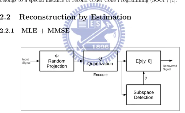
Figure 2.1: Recover the signal through estimation

In (2.2), the reconstruction of x can be cast as an estimation problem, in which the parameters of interest are the subspace of non-zero coefficients, i.e., the sparsity pattern, and their values. This approach usually involves assuming a probabilistic model for both signal subspace θ and non-zero coefficients w ∈ ℜS_{. For example, Fletcher et}

uniformly in [1, CN

S]; in addition, w is independent of θ. With their models, the sparse

signal x is given by

x= Ψθw, (2.7)

where Ψθ is composed of column vectors in Ψ that correspond to non-zero elements in u.

Substituting (2.7) into (2.2) gives y = ΦΨθw. Taking into account quantization effects,

we then have a simple linear additive noise model,

˜

y= ρΦΨθw+ n, (2.8)

where the quantization noise vector n ∼ N (0, Cn) and ρ is the linear gain of forward

quantization model. To estimate θ, Fletcher et al. [4] employed the ML technique to identify sparsity pattern, leading to a

ˆ

θ = max

j=1,..,CN

S

kPjyk,˜ (2.9)

Define the asymptotic probability of subspace mis-estimation as Perr = limN →infP r(ˆθ 6=

θ), the ratio sparsity to the measurement number α = _MS, and the quantization accuracy β= 2−_2αR

. While there are sufficient bit-rate R to allow α and β satisfying

−1 2log2(β) ≥ αRV + 1 2αlog2(1 + 1 − β αβ ) (2.10) then Perr will act like a step function,

Perr =

(

1, α > αcrit

0, α < αcrit (2.11)

meanwhile, with ˆθ, x is further inferred using the MMSE estimate.

ˆ

x= E[x|˜y, θ= ˆθ] (2.12)

It is expected that the estimation approach can use fewer measurements to reconstruct x than the l1 algorithm. Essentially, this is because the latter does not use any prior

knowledge of the source. Our simulation results, as given in Chapter 3, show that the former requires approximately half of the measurements necessary for the l1 decoding.

2.2.2

Asymptotic R-D Performance

The motivation of compressive sensing is that the sensing matrices and sparsity pat-terns are not known by the encoder; instead, they are only known by the decoder. To further study the limitation of CS rate-distortion performance, Fletcher et al. evaluated the performance of a simple but non-universal compression scheme, allowing both the encoder and decoder to know the sensing matrices and sparsity patterns. Since now the encoder can adapt to the signal structure, they call this scheme adaptive quantization. In the case, the encoder is simply quantizing a S-dimensional Gaussian random vector with given RS bits. By the well-known rate-distortion function for a Gaussian source,

DGaussian(R) = 2−2R. (2.13)

Of course, for sparse signal, the sparsity pattern θ is unknown, hence the encoder has to spend log₂J bits for encoding J possible sparsity patterns. Let

RV =

1

Slog2J, (2.14) Therefore, the distortion of adaptive quantization can be shown as,

Dadapt(R) =

(

2−_2(R−RV)

, R > RV;

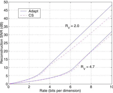
1, otherwise. (2.15) To illustrate the relationship between compressive sensing and adaptive quantization on the basis of rate-distortion performance, Fletcher et al. plot the asymptotic distor-tion for both. Fig. 2.2 displays the distordistor-tion as a funcdistor-tion of quantizadistor-tion rate R, for different subspace rate RV = 2 and 4.6, showing the main important findings: the

recon-struction SNR can be increased with lower subspace rate RV, since adaptive quantization

needs fewer bits to encode the subspace index. Therefore, compressive sensing is possible to achieve the similar performance with adaptive quantization, if the priori was used in decoding. However, there are some questions raised: Firstly, is it possible to use fewer measurements in decoding CS measurements through estimation-based approach? Sec-ondly, if the answer is affirmative, can we consider the 2-step approach (MLE + MMSE) as a promising decoding method? These questions will be answered in Chapter 3.

Figure 2.2: Asymptotic performance of compressive sensing(CS) and adaptive quantiza-tion(Adapt) of a sparse source

2.3

Related applications of compressive sensed

im-ages

In this chapter, we will introduce the applications of compressive sensing, including image compression and multiple description coding.

2.3.1

Compressively Sampled Images

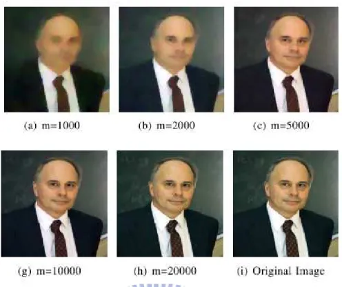
Jafarpour et al. [2] select a variety of different real images to test the quality of the recovered images. Instead of using l1 minimization in recovering the sparse represented

images in the wavelet domain, they used a quadratic programming method called min T V. Following is its definition,

|x|T V =

X

i,j

q

(xi+1,j − xi,j)2+ (xi,j+1− xi,j)2 (2.16)

By using (2.16), the original linear programming (2.3) can be cast as a min TV recovering algorithm,

ˆ

Figure 2.3: Recover the image by min TV with different measurement number

As we can see from Fig. 2.3, the T V method is an efficient way to recover a two dimensional piecewise smooth signal, for example, natural images. Therefore, many ap-plications prefer to use T V method rather than l1 minimization in image reconstruction

for enhancing the subjective quality. Although such recovering algorithm is restricted to a specific type of signals, and it doesn’t promise the exact reconstruction as l1, Total

Variance still provides a key concept that CS decoding can benefit from using some prior knowledge of the signal.

2.3.2

Compressive Sensing based Multiple Description Coding

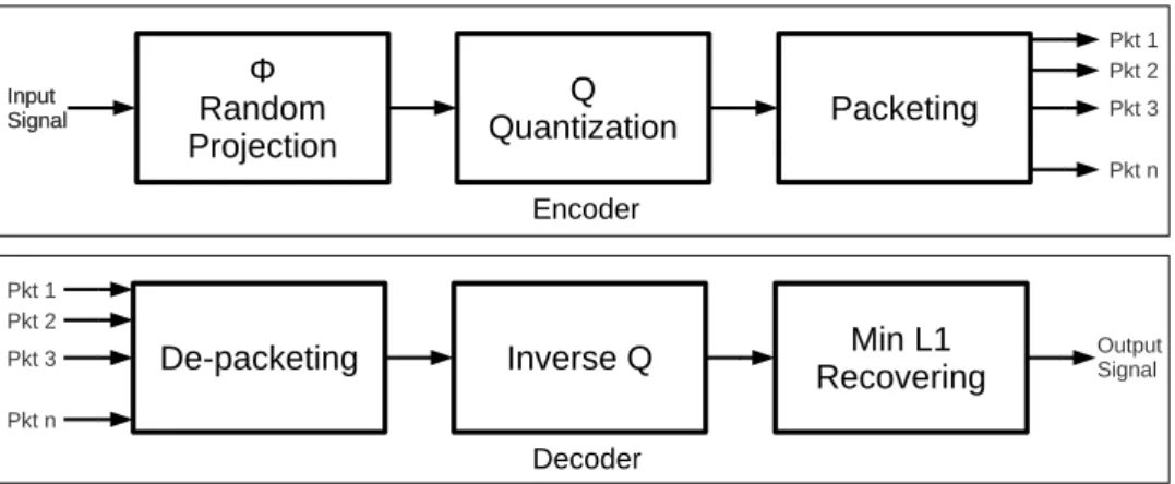
Among present CS-MDC architecture [3] [7], the common framework is based on the scheme of random projection and l1 minimization, as shown in Fig. 2.4. In this

frame-work, the image is fragmented into multiple blocks, and then projected into CS random measurements. After receiving these measurements, encoder will de-fragment all the re-ceived measurements and recover the signal through l1 minimization by equation (2.6).

Because different measurements are equally important, the decoding quality only depends on the received measurement number.

Figure 2.4: Present CS-MDC system

Another issue is controlling the number of transmitted measurements, which affects the compression efficiency. Based on an empirical distortion function [3] [9] e(M ) = βM−_δ

for l1 algorithm, the transmitted measurement number can be decided by setting

a target distortion. However, not matter in our study or the prior works in [4], the distortion behavior of estimation-based frameworks are not identical with the l1algorithm.

Therefore, the measurement allocation should be discussed again, instead of using the empirical distortion function for l1. This work can be found in the Chapter 6.

Chapter 3

MAP Decoding Algorithm

The mis-estimation of θ has a profound effect on the reconstruction quality. It may provide a wrong prior information for estimating x, as suggested by (2.12); moreover, the misplace of non-zero coefficients often induces significant distortion. It was shown in [4] that the ML estimator in (2.9) has an error probability that is a step function of the ratio of sparsity S to measurement number M : the probability of error flips suddenly from 0 to 1 if the ratio exceeds a critical threshold. This is due in part to the ignorance of the prior information of w. To overcome this problem, we propose a MAP decoding scheme that make use of the prior knowledge of both θ and w for a joint estimation. Their estimators are then substituted into (3.7) to predict x. It turns out that (3.7) has the same form as (2.12), except that the θ estimator is different, as we now proceed to show.

3.1

MAP Estimators for Sparsity Pattern and

Non-zero Coefficients

To jointly estimate θ and w on the basis of ˜yby the MAP rule, we need the posterior distribution. Since θ is discrete but w is continuous, we define the posteriori to be maximized as

P(θ, w′

≤ w < w′

where {w′

≤ w < w′

+ ∆w} is an event and ∆w ∼ 0 is a fixed, small displacement. The

MAP estimators are thus the values of θ and w′

that maximize P(θ, w′ ≤ w < w′ + ∆w|˜y) = P (θ|˜y)P (w′ ≤ w < w′ + ∆w|θ, ˜y) = P (θ|˜y)f (w′ |θ, ˜y)∆w = P(θ)f (˜y|θ) f(˜y) f(w ′ |θ, ˜y)∆w = P(θ)f (w ′ |θ)f (˜y|w′ , θ)∆w f(˜y) , (3.2)

where the last equality is because f (˜y, w′

|θ) = f (˜y|θ)f (w′

|θ, ˜y) = f (w′

|θ)f (˜y|w′

, θ). The conditional probability density function (pdf) f (˜y|θ, w′

) can be further computed, using (2.8) and the signal models in [4], as

f(˜y|θ, w′ ) = 1 (2π)M/2_det(C n) e−1 2(˜y−Hθw′) T_C−1 n (˜y−Hθw′)_{. (3.3)}

Since θ and w have uniform and Gaussian distributions, respectively, we then arrive at

(ˆθ,w) = minˆ θ,w′{(˜y− Hθw ′ )TC−₁ n (˜y− Hθw′) + (w′− uw)TC−w1(w ′ − uw)}, (3.4)

The search for θ and w in (3.4) need not be exhaustive. Observe that if θ is fixed, the objective is an unimodal, convex function in w. Thus the relation between ˆw and θ must satisfy ˆ w= uw+ (C −₁ w + HθTC −₁ n Hθ) −₁ H_θTC−₁ n (˜y− Hθuw), (3.5)

which is exactly the conditional mean E[w|˜y, θ]. A back substitution of (3.5) into (3.4) gives ˆ θ= min θ {(˜y− Hθw)ˆ T_C−1 n (˜y− Hθw) + ( ˆˆ w− uw)TC−w1( ˆw− uw)}, (3.6)

Note that a numerical search for ˆθ is inevitable since θ is discrete. With both ˆθ and ˆw, we give an estimate of x by

ˆ

x= Ψ_θˆwˆ (3.7)

It is instructive to remark on the differences between our estimators and those in [4]. Firstly, if (3.7) is used to give an estimate of x, it has the same form as that in (2.12).

Proof. ˆ x = E[x|y, θ = ˆθ] = E[Ψθw|y, θ = ˆθ] = Ψ_θˆE[w|y, θ = ˆθ] = Ψ_θˆwˆ

This is because ˆw = E[w|˜y, θ = ˆθ] and Ψθ is a matrix with orthonormal columns.

It then follows that the MMSE estimator commutes over linear transformation of w. Secondly, our θ estimator involves the prior information of w, which is a consequence of the joint estimation. Given the additional information, it is expected to outperform the ML estimator in (2.9), as will be verified subsequently.

3.2

Performance Analysis

In this section, we carry out a number of experiments to verify the performance of our MAP estimators, which is compared to that of the l1 algorithm and of the 2-step approach

[4]. The first experiment examines their decoded distortion versus measurement number, mainly to understand the effect of insufficient measurements on reconstruction quality. The second experiment analyzes the average measurement number needed for achieving a specified distortion level, in order to assess the R-D performance when measurement number can be communicated to the decoder for each signal realization, as is common in many practical applications. In both experiments, we generate the source using the signal assumptions in [4], that is, w ∼ N (0, σ2_{I) and θ ∼ U[1, C}N

S], with sparsity S = 16 and

signal dimension N = 64. The results shown are on the basis of 10,000 (independent) simulation runs.

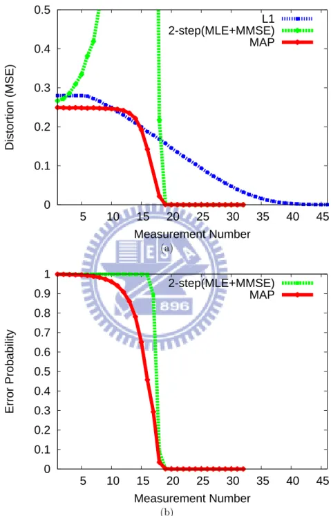
Fig. 3.1(a) plots the mean squared reconstruction errors of all three schemes as func-tions of measurement number. As expected, to achieve perfect reconstruction, the l1

algo-rithm requires a significantly larger number of measurements than the other two schemes. Amazingly, the number required for the latter two schemes is very close to the sparsity value, indicating the minor overhead necessary for signaling the positions of non-zero

coef-ficients. This also demonstrates the benefits of introducing prior information in decoding. Another interesting observation is that the 2-step approach has a much higher distortion than the other schemes, when the measurement number drops below the sparsity. To give reasons, Fig. 3.1(b) shows the error probabilities of the sparsity pattern θ. It can be seen that the MAP estimator has a uniformly smaller error probability than the ML estimator, although the difference is negligible given extremely insufficient measurements (e.g. 5-15). It is worth pointing out that the mis-estimation of θ will affect the estimation of x through (2.12). Such chain effect may cause the ML estimator to produce a distor-tion that is even higher than using prior mean ˆx = 0, especially when the measurement number is insufficient. This is corroborated by the comparison with the l1 algorithm, for

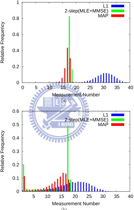
which we use prior mean as the estimate of x whenever it fails to recover the signal. The analysis in Fig. 3.1(a) applies a fixed number of measurements to all signal re-alizations. Even though the sparsity is fixed, it is seen in many cases and for all three schemes that some signals can be reconstructed with much fewer measurements than others. Motivated by this observation, we provide in Fig. 3.2 the distributions of mea-surement number needed for the three algorithms to achieve perfect reconstruction. It is not surprising that when ordered by the average number, these algorithms have a relation of l1 >2-step > MAP. But, what is new is that the l1 algorithm also has a larger variance

due to its universal property. Recall that it makes no use of any prior information, other than the premise that signal is sparse. In Fig. 3.2(b) the analysis is further extended to the case with distortion (MSE=0.06). We see that the distribution of the l1 now become

woven together with the other two, in which the one of our MAP scheme spreads out more towards zero. These results have two implications. The first is that when used for perfect reconstruction, the l1 is far from efficient: relaxing a bit the quality constraint

yields a significant saving of measurements. The second is compatible with our previous finding; that is, our scheme can better recover the signal with fewer measurements due mainly to its improved accuracy in estimating sparsity pattern.

In summary, our analysis reveals that the l1 algorithm is universal, but, as it is, far

should be used to their best advantage. The 2-step and the MAP approaches are two examples showing how the priors could possibly be utilized at the decoder. In both approaches, the fidelity of sparsity pattern has a great influence on decoded quality and our MAP scheme is shown to outperform the ML estimator.

0 0.1 0.2 0.3 0.4 0.5 5 10 15 20 25 30 35 40 45 Distortion (MSE) Measurement Number L1 2-step(MLE+MMSE) MAP (a) 0 0.1 0.2 0.3 0.4 0.5 0.6 0.7 0.8 0.9 1 5 10 15 20 25 30 35 40 45 Error Probability Measurement Number 2-step(MLE+MMSE) MAP (b)

Figure 3.1: The measurement-distortion curves of various decoding algorithms (a) and their error probabilities of sparsity pattern (b)

0 0.2 0.4 0.6 0.8 1 0 5 10 15 20 25 30 35 40 Relative Frequency Measurement Number L1 2-step(MLE+MMSE) MAP (a) 0 0.1 0.2 0.3 0.4 0.5 0.6 5 10 15 20 25 30 35 40 Relative Frequency Measurement Number L1 2-step(MLE+MMSE) MAP (b)

Figure 3.2: Measurement number distribution subject to distortion constraints: (a) MSE=0 and (b) MSE=0.06.

Chapter 4

Compressive Sensing with Bit-Plane

Separation

4.1

Concept of Bit-Plane Separation

As we saw earlier, it is important to minimize the error probability of sparsity pattern Pe(θ). Unfortunately, given an insufficient measurement number, this probability tends

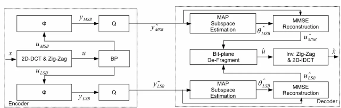
to one in most decoding algorithms. This explains why their distortions usually remain unchanged in the low-rate region. To maximize the probability of correct decision while minimizing the required measurement number, we introduce the notion of bit-plane (BP) separation in the CS framework. Fig. 4.1 illustrates the concept of operations. As shown, the sparse signal representation u is first partitioned into a MSB BP and a LSB BP by a scalar quantizer and then the resulting signals are sampled independently by CS. Observe that the MSB signal uM SB, which captures most significant information about

u, usually has a higher sparsity than the original signal u. In anticipating that uM SB can

be recovered first with few measurements, we expect the BP separation to help improve R-D performance, especially in the low-rate region. However, this approach, like two-layer scalable coding, may also introduce redundancy in the high-rate region. In this chapter, we shall analyze this new framework in detail.

4.2

Performance Analysis

We start with the R-D comparison in Fig. 4.2(a), where the horizontal axis indicates rate constraint (expressed in number of bits) rather than measurement number. Note that

Figure 4.1: Concept of operations for bit-plane CS.

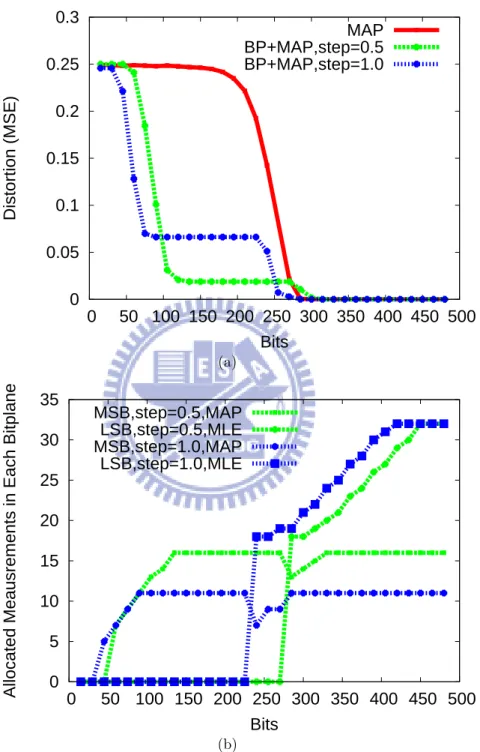
measurement fidelity for different configurations is not uniform: without BP separation, each measurement is quantized uniformly into 15 bits, while with BP separation, the measurements at the MSB and the LSB BPs have a precision of 8 bits and 10 bits, respectively. These numbers are so chosen that the SNR ratio is high enough for almost lossless signal reconstruction. Fig. 4.2(a) confirms our prediction. As expected, the distortions associated with using BP separation drop drastically in the low-rate region. Inspection of Fig. 4.2(b) reveals that this is because the MSB BP is allocated with all measurements available, which is intuitively agreeable since the LSB BP can hardly contribute to distortion reduction with only few measurements due to its low sparsity.

Another interesting observation is seen by noting that the distortions remain at a fixed level in the mid-rate range. According to Fig. 4.2(b), neither the MSB BP or the LSB BP is allocated with more measurements. These are the points at which the MSB signal has been perfectly reconstructed, but the number of measurements is still far from sufficient to recover the LSB. Remarkably, our θ estimator for the LSB BP become the ML estimator, i.e., (2.9), since its non-zero coefficients wLSB tend to have a uniform distribution. It is

thus conceivable that the best policy is not to allocate any measurements to the LSB: recall that the ML estimate may result in a higher distortion than prior mean, given insufficient measurements.

As the rate is increased further, we observe a sudden increase in the LSB measure-ment number along with a slight decrease in the MSB measuremeasure-ment number. This is a manifestation of the step-like R-D behavior of the ML estimator. The transition indi-cates the borderline between the perfect reconstruction and the complete corruption of

the LSB signal, at which sacrificing a bit the MSB quality is more R-D efficient in the present example. The degradation extent depends on the quantization step size used for BP separation.

The results so far have an important implication: the conventional CS framework is far from ideal for signal compression. Although using BP separation helps to improve its R-D performance, the technique is quite arbitrary and by no means optimal. There is still plenty of room for further improvement.

0 0.05 0.1 0.15 0.2 0.25 0.3 0 50 100 150 200 250 300 350 400 450 500 Distortion (MSE) Bits MAP BP+MAP,step=0.5 BP+MAP,step=1.0 (a) 0 5 10 15 20 25 30 35 0 50 100 150 200 250 300 350 400 450 500

Allocated Meausrements in Each Bitplane

Bits MSB,step=0.5,MAP LSB,step=0.5,MLE MSB,step=1.0,MAP LSB,step=1.0,MLE (b)

Figure 4.2: The effect of bit-plane separation on the R-D performance: (a) R-D curves and (b) measurement allocation.

Chapter 5

Application to Image Compression

In this chapter, we apply the previously developed estimators to image compression. Following the common practices, we divide an image into 8x8 blocks, each of which, when spanned by DCT basis, approximates a sparse signal. In this case, the DCT coefficients form the sparse representation. For its BP separation, the quantization step size is set to 128, and the MSB and LSB BPs are properly quantized into 8 bits and 11 bits, respectively, compared to 12 bits without BP separation. In addition, uwand Cw in 3.5 are substituted

with their minimum variance unbiased estimators, since both are unknown for real image data.

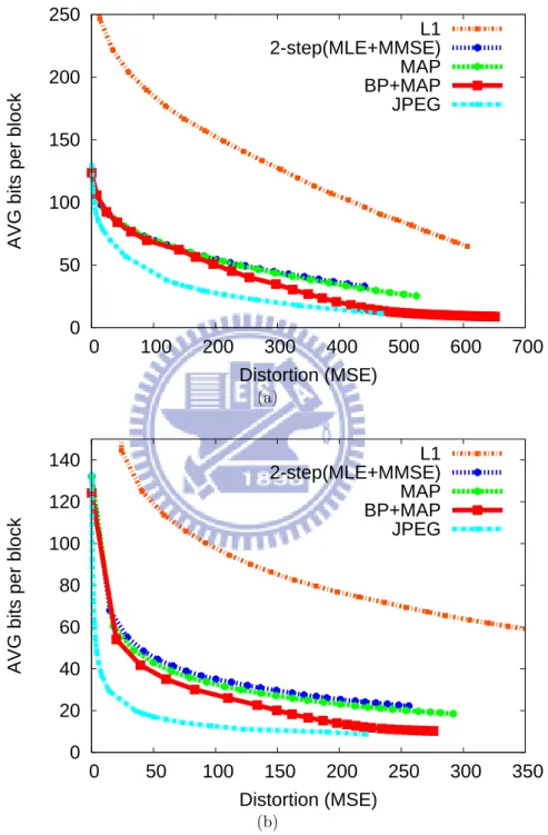
Fig. 5.1 compares the R-D curves of various decoding schemes. Particularly, the average number of bits per block are displayed as functions of distortion. This is to account for the use of CS in many practical situations, where the decoder is usually informed of the minimum measurement number required for each signal realization. From Fig. 5.1, the results are mostly in agreement with theoretical simulations, although our signal models may not best represent real data. As expected, the use of prior information always improves estimation accuracy and the benefit of BP separation is most obvious when only few measurements are available. However, to our surprise, the 2-step approach is not that pessimistic, as compared with our scheme. This is attributed to that measurement number can now be chosen properly to suit the need of each block. With reference to Fig. 3.2, their means indeed tend to be identical, even though the distributions differ significantly. The comparison with JPEG further shows the promising aspect of our scheme. The difference in compression ratio (given the same image quality) is seen to

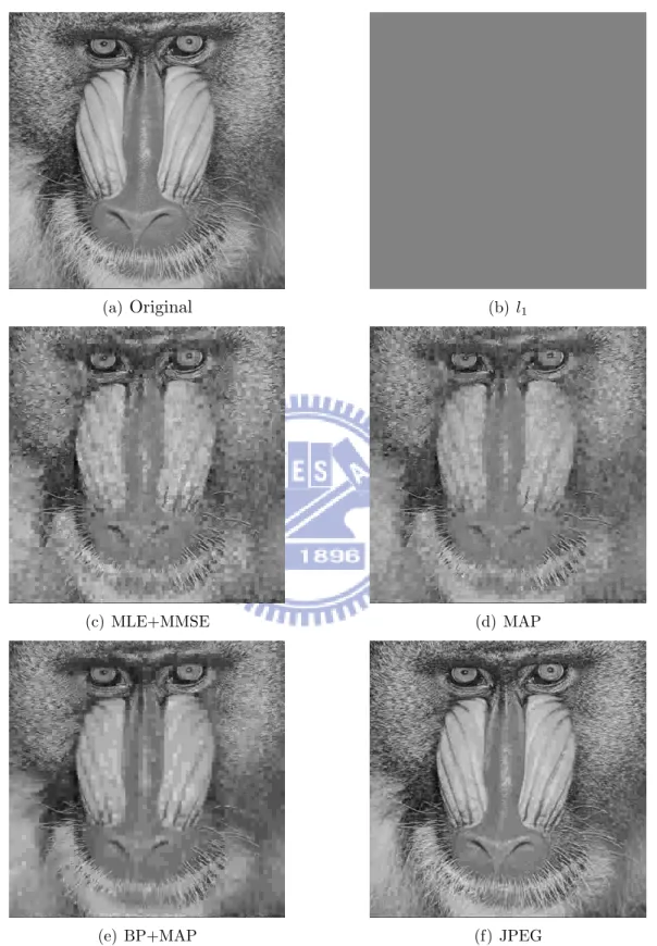
be within a factor of two. Fig. 5.2 and 5.3 provide sample results of subjective quality comparison.

0 50 100 150 200 250 0 100 200 300 400 500 600 700

AVG bits per block

Distortion (MSE) L1 2-step(MLE+MMSE) MAP BP+MAP JPEG (a) 0 20 40 60 80 100 120 140 0 50 100 150 200 250 300 350

AVG bits per block

Distortion (MSE) L1 2-step(MLE+MMSE) MAP BP+MAP JPEG (b)

(a) Original (b) l1

(c) MLE+MMSE (d) MAP

(e) BP+MAP (f) JPEG

Figure 5.2: Baboon, average bpp=0.52, PNSR : (a) inf (b) fail (c) 21.726 (d) 22.032 (e) 23.427 (f) 26.263

(a) Original (b) l1

(c) MLE+MMSE (d) MAP

(e) BP+MAP (f) JPEG

Figure 5.3: Lena, average bpp=0.47, PNSR : (a) inf (b) fail (c) 26.428 (d) 27.360 (e) 28.97 (f) 57.924

Chapter 6

Application to Multiple Description

Coding

Compressive sensing is a natural tool to realize the multiple description coding, when CS measurements are treated as MDC descriptions. However, most existing CS-MDC don’t use any prior knowledge about the image in reconstruction; instead, they use the l1 and T otalV ariance to recover the signal. As a consequence, these decoding methods

are not promised in the case of insufficient measurements, as compared with our MAP decoding algorithm. To adapt the MAP framework in Fig. 4.1 into a MDC system, we have to concern about the problem of measurement allocation.

6.1

Measurement Allocation

Fig. 3.2 suggests that uniform allocation of the measurements is not optimal; in other words, the allocation of measurements should be variant with different blocks. Given a block that can be perfectly represented with k measurements. If each measurement was transmitted through an erasure channel with loss probability p, i.i.d, then we can acquire the failure rate for transmitting m measurements, define

Pf ailure:= P (number of received measurements < k) (6.1)

Then the failure rate can be derived as a binomial cumulative distribution function,

Pf ailure(m) =

k−1

X

i=0

C_im(1 − p)i(p)m−i (6.2)

Due to the fact that Pf ailure(m) is a decreasing function of m, where m can be found

Figure 6.1: Concept of operations for bit-plane CS-based MDC.

can be formally elaborated as a minimization process,

minimize mi Pf ailure(mi) subject to X i mi× R ≤ Rtarget mi ≥ ki (6.3)

where i is an index to indicate different blocks.

6.2

Pseudo-Random Packetization

To promise the measurements of every blocks can be received by a certain proportion, a pseudo uniformly-random packeting approach is used in our system. Given P packets that should be transmitted by encoder, each measurement will be assigned to the packet through a mapping function P kt(y_jq) = rand(j) mod P , where j is the index of each measurement. Therefore, both encoder and decoder can coherently generate the same pseudo random sequence, avoiding the overhead of synchronization. The whole system is given in Fig. 6.1, depicting the operations in the case of losing packets.

6.3

Performance Analysis

In this experiment, most of settings are inherited from previous chapter, e.g. quanti-zation bits, signal models, etc. The allocated measurements are also divided into P = 100 packets to meet the realistic application, and an erasure channel is also simulated with different loss rate (10%-90%). To do the adaptive measurement allocation through (6.3), the CS-MDC system is restricted to achieve a compression ratio = 1.5 for satisfying the

rate constraint Rtarget, and the loss rate is set to p = 0.6(60%) for deciding the failure

rate through (6.2). Meanwhile, we also compare our adaptive approach with an intuitive linear allocation framework, allowing us to justify the necessary of adaptive allocation. the operation of linear allocation is easy to be shown as,

E[received measurements] = mi(1 − p) ≥ ki

⇒ mi ≥

ki

1 − p = c · ki (6.4) The relation between mi and ki in (6.4) tends to be linear dependent with a coefficient c,

seems easier and more intuitive than the adaptive strategy in (6.3). Therefore, a question is raised whether it can achieve the same or even better performance than our adaptive strategy? The answer is negative, because linear allocation is based on the ”mean” sense, decoder may fail in recovering some blocks that lost too many measurements. This result can be shown in our simulations.

Fig 6.2 displays the distortion as a function of loss rate. As we saw in other prior works, distortion of l1 exhibits an exponentially increased function of loss rate.

Amaz-ingly, the performance of 2-step (MLE+MMSE) is even worse than the l1 recovering

algorithm, whose distortion is significantly higher than the other approaches. To give reasons, recall that the 2-step approach will suffers subspace mis-estimations from insuf-ficient measurements, resulting in very high distortion, as shown in Fig. 4.2. Therefore, the 2-step approach is not an ideal solution for coping with erasure channel, due to the sensitivity of measurement number. As we can predict, MAP-based CS-MDC provides an outstanding recovering performance, owing to its better estimation of subspace. Be-sides, the integration of bit-plane separation doesn’t bring any obvious pros or cons to the error-resilience, hence the bit-plane separation is simply a way to enhance the compres-sion ratio without sacrificing the functionality of error-resilience. However, if the adaptive allocation is replaced by the linear approach, the performance degradation can be easily observed. In conclusion, MAP-based algorithm with adaptive measurement allocation allows CS-MDC to achieve a much better compression efficiency and provide stronger error-resilience, rather than conventional l1-based algorithm. Fig. 6.3 - 6.8 shows the

0 500 1000 1500 2000 10 20 30 40 50 60 70 80 90 100 Distortion (MSE)

Packets Loss Percentage L1

2-step(MLE+MMSE) MAP BP+MAP (Linear Allocation) BP+MAP (a) 0 500 1000 1500 2000 10 20 30 40 50 60 70 80 90 100 Distortion (MSE)

Packets Loss Percentage L1

2-step(MLE+MMSE) MAP BP+MAP (Linear Allocation) BP+MAP

(b)

Figure 6.2: Loss - Distortion performance subject to compression ratio = 1.5 (a) Baboon and (b) Lena.

(a) Original (b) l1

(c) MLE+MMSE (d) MAP

(e) BP+MAP (Linear Allocation) (f) BP+MAP

Figure 6.3: Baboon, compression ratio=1.5 ,loss rate = 40% , PNSR : (a) inf (b)33.60 (c)74.74 (d)74.66 (e)33.05 (f)65.27

(a) Original (b) l1

(c) MLE+MMSE (d) MAP

(e) BP+MAP (Linear Allocation) (f) BP+MAP

Figure 6.4: Baboon, compression ratio=1.5, loss rate = 60% , PNSR : (a) inf (b)24.09 (c)17.3719 (d)36.52 (e)26.76 (f)28.63

(a) Original (b) l1

(c) MLE+MMSE (d) MAP

(e) BP+MAP (Linear Allocation) (f) BP+MAP

Figure 6.5: Baboon, compression ratio=1.5, loss rate = 80%, PNSR : (a) inf (b)14.17 (c)fail (d)19.37 (e)18.59 (f)20.59

(a) Original (b) l1

(c) MLE+MMSE (d) MAP

(e) BP+MAP (Linear Allocation) (f) BP+MAP

Figure 6.6: Baboon, compression ratio=1.5, loss rate = 40%, PNSR : (a) inf (b)31.63 (c)74.45 (d)74.40 (e)30.99 (f)81.39

(a) Original (b) l1

(c) MLE+MMSE (d) MAP

(e) BP+MAP (Linear Allocation) (f) BP+MAP

Figure 6.7: Baboon, compression ratio=1.5, loss rate = 60%, PNSR : (a) inf (b)23.52 (c)fail (d)37.66 (e)24.06 (f)37.61

(a) Original (b) l1

(c) MLE+MMSE (d) MAP

(e) BP+MAP (Linear Allocation) (f) BP+MAP

Figure 6.8: Baboon, compression ratio=1.5, loss rate = 80%, PNSR : (a) inf (b)12.39 (c)fail (d)20.72 (e)18.36 (f)23.57

Chapter 7

Conclusion

In this thesis, we derived the MAP estimator from a theoretical model, and empirically analyzed its R-D performance. Meanwhile, we also proposed a technique of bit-plane separation that can further improve the R-D performance of CS. Our study obtains the following discoveries:

1. The CS R-D behavior highly depends on the decoding algorithm, instead of encoding method. As we can see from the empirical R-D performance, the one using the priori can significantly reduce the distortion rather than the blind approach, given the identical encoding scheme and same number of measurements.

2. Our MAP method shows a promising result, even with insufficient measurements. This is because MAP has a better estimate of the signal subspace, providing a much better reconstruction than ML+MMSE does. By incorporating signal prior knowledge for decoding, MAP can reconstruct a sparse signal perfectly with a mea-surement number very close to its sparsity.

3. To further improve R-D performance, a technique of bit-plane separation is proposed and combined with our MAP estimator. Due to the high sparseness of MSB bit-plane, MAP can recover the MSB bit-plane with very few measurements. Therefore, it can be anticipated that the distortion can be further minimized in the low rate region, since the limited bit-rate is enough to allocate sufficient number of MSB measurements.

achieve a promising results as compared with the well-optimized JPEG codec. Meanwhile, due to a better reconstruction quality with highly insufficient measure-ments, MAP is also an efficient decoding algorithm on the application of MDC.

Our work is still in its early stage, we plan to extend our investigation in several directions:

1. The MAP decoding algorithm should be analyzed theoretically. As we observed from the simulation results, MAP is possible to recover the signal with a measurement number that is even below the sparsity. Such interesting fact should be further studied.

2. Bit-plane separation is very intuitive and by no means optimal; however, it still enhance the the R-D performance of CS. This result implies that the existing CS encoding framework is not very efficient. A question arises whether there exists an optimal coding technique that can be used in CS encoding.

3. During our investigation of Bayesian MAP decoding framework, another CS frame-work is also proposed by Shihao Ji et al., named as ”Bayesian Compressive Sens-ing” [10]. It should be noticed that their approach is based on ”Bayesian Machine Learning”, and hence such framework is implemented by the Relevance Vector Ma-chine algorithm. Although Bayesian learning also involves the using of priori, their work did not show such amazing improvement as we did. Therefore, it is very in-teresting to study the difference between theirs and ours, for further investigating a better way of applying Bayesian inference to CS.

Bibliography

[1] E. J. Candes, “Compressive sampling,” in Int. Congress of Mathematicians, Madrid, Spain,, Aug. 2006.

[2] S. Jafarpour, A. Pezeshki, and R. Calderbank, “Experiments with compressively sampled images and a new debluring-denoising algorithm,” in IEEE International Symposium on Multimedia, 15-17 2008, pp. 66 –73.

[3] L. J. Wang, X. L. Wu, and G. M. Shi, “A compressive sensing approach of mul-tiple descriptions for network multimedia communication,” in IEEE Workshop on Multimedia Signal Processing, 2008.

[4] A. K. Fletcher, S. Rangan, and V. K. Goyal, “On the rate-distortion performance of compressed sensing,” in IEEE Int. Conf. on Acoustics, Speech and Signal Processing, 2007, vol. 3.

[5] V. K. Goyal, A. K. Fletcher, and S. Rangan, “Compressive sampling and lossy compression,” IEEE Signal Processing Magazine, vol. 25, no. 2, pp. 48–56, March 2008.

[6] V. K. Goyal, “Multiple description coding: Compression meets the network,” IEEE Signal Processing Magazine, vol. 18, no. 5, pp. 74–93, Sep 2001.

[7] Y. f. Zhang, S. L. Mei, Q. Q. Chen, and Z. B. Chen, “A multiple description image/video coding method by compressed sensing theory,” in IEEE Int. Symposium on Circuits and Systems, 2008.

[8] E.J. Candes, J. Romberg, and T. Tao, “Robust uncertainty principles: exact signal reconstruction from highly incomplete frequency information,” IEEE Transactions on Information Theory, vol. 52, no. 2, pp. 489 – 509, feb. 2006.

[9] J. Haupt and R. Nowak, “Compressive sampling vs. conventional imaging,” in IEEE International Conference on Image Processing, 8-11 2006, pp. 1269 –1272.

[10] S. H. Ji, Y. Xue, and L. Carin, “Bayesian compressive sensing,” IEEE Trans. on Signal Processing, vol. 56, no. 6, pp. 2346–2356, June 2008.