國 立 交 通 大 學
電 信 工 程 學 系
碩 士 論 文
在無線區域網路中
使用擴展性混和協調功能控制型通道存取方式
保證服務品質
Scalable HCCA Scheduler for QoS Guarantee
in IEEE 802.11e WLANs
研 究 生 : 葉家豪
指導教授 : 李程輝 博士
在無線區域網路中
使用擴展性混和協調功能控制型通道存取方式
保證服務品質
Scalable HCCA Scheduler for QoS Guarantee
in IEEE 802.11e WLANs
研 究 生 : 葉家豪 Student: Chia-Hao Yeh 指導教授 : 李程輝 博士 Advisor: Dr. Tsern-Huei Lee
國 立 交 通 大 學 電 信 工 程 學 系 碩 士 班
碩 士 論 文
A Thesis
Submitted to Department of Communication Engineering College of Electrical and Computer Engineering
National Chiao Tung University in Partial Fulfillment of the Requirements
for the Degree of Master of Science in Communication Engineering June 2009 Hsinchu, Taiwan
中 華 民 國 九 十 八 年 六 月
Chinese Abstract
在無線區域網路中
使用擴展性混和協調功能控制型通道存取方式
保證服務品質
學生: 葉家豪 教授: 李程輝國立交通大學電信工程學系碩士班
中文摘要
在 IEEE 802.11e 的媒體存取控制中定義了一個新的通道存取機制, Hybrid Coordination Function(HCF),分配傳送機會(TXOP)給符合服務 品質(QoS)需求的工作站。IEEE 802.11e 規格定義的 HCF 控制型通道存 取控制(HCCA)參考排程器(Sample Scheduler),傳送機會的計算是採用 平均資料速率對於變動位元速率(Variable Bit Rate)的封包並不適用。一 種預測和最佳化控制型通道存取方式(PRO-HCCA)被提出用來處理變 動位元速率的封包,把訊務流(Traffic Stream)的延遲限制(Delay Bound) 列入考慮,相較於參考排程器,能保證較佳的服務品質。在預測和最 佳化控制型通道存取方式排程中,每個訊務流是獨立被輪詢(Polling), 導致有較多的輪詢額外負擔(Overhead)。因此,我們提出了一個修改的 機制,每個工作站獨立被輪詢,接著使每個工作站分別有不同的輪詢 週期,模擬結果指出我們的方法不但可以達到服務品質的需求,對於 頻寬的使用效率上也比預測和最佳化控制型通道存取方式來的好。English Abstract
Scalable HCCA Scheduler for QoS Guarantee
in IEEE 802.11e WLANs
Student : Chia-Hao Yeh Advisor : Tsern-Huei Lee Institute of Communication Engineering
National Chiao Tung University
Abstract
The Medium Access Control of IEEE 802.11e defines a novel coordination function, namely, Hybrid Coordination Function (HCF), which allocates Transmission Opportunity to stations taking their quality of service (QoS) requirements into account. A sample scheduler was provided for HCF Controlled Channel Access (HCCA), a contention-free channel access function of HCF. The sample scheduler is not suitable for VBR traffic because delay bounds are not considered in TXOP allocation. A prediction and optimization-based HCCA (PRO-HCCA) scheduler, which takes delay bounds of different traffic streams into consideration, has recently been proposed to handle VBR traffic. PRO-HCCA was shown to provide much better QoS guarantee than the sample scheduler. The granularity of PRO-HCCA is per traffic stream which causes scalability issue. Besides, each traffic stream is polled individually in every service interval, which implies considerable overhead. Therefore, we present a modified scheme that has per-station granularity and thus is more scalable than PRO-HCCA. To reduce polling overhead, we further modify the scheduler so that different stations can have different polling periods. Numerical results show that our proposed schemes meet QoS requirements and utilize bandwidth more efficiently than PRO-HCCA.
Acknowledgement
誌謝
感謝指導教授─李程輝老師,兩年來的指導,讓我在每次的開會、 私下的討論和待人處事方面都獲益良多,老師和我們間詼諧的對答讓 我發現到原來師生間可以這麼的零距離。 感謝親愛的爸爸、媽媽,從小給予我正當的教導,以及精神上的 鼓勵,使我能勇往直前朝自己的興趣發展,感謝我兩位活潑的姐姐當 我的好榜樣,讓我在求學生活中一直有目標和動力,謝謝我家的愛狗 奧斯卡陪著我們一家人十五年,因為有你家裡更加歡樂。 感謝景融學長和郁文學長在無線網路組給了我很多細心的指導和 建議,感謝學長姐─迺倫、瑋哥、歪歪、CC 大、世弘、凱文、鑫哥、 北極,讓我在懵懂的碩一時期能快速的進入狀況。謝謝同屆夥伴們─ 佑信、大頭、松晏、鈞傑、小汪、BBN、堯堯,在課業上和生活上都 能一起相互扶持。謝謝學弟妹們─小机、小薇、假菜、韋儒、熊仔、 世倫,因為有你們的加入,實驗室充滿了歡樂。 謝謝元智大學一起準備研究所的戰友們,當初一起在圖書館奮 鬥,成立讀書會,大家最終都考上自己心目中理想的學校,打破電機 系有史以來研究所成績最優異的一屆。 謹將此論文獻給所有我愛與愛我的人。 2009 年 6 月於風城交大Contents
Contents
中文摘要 ... I ABSTRACT ... II 誌謝 ... III CONTENTS ... IV LIST OF TABLES ... VI LIST OF FIGURES ... VI CHAPTER 1. INTRODUCTION ... 1CHAPTER 2. RELATED WORK ... 4
2.1. SYSTEM MODEL ... 4
2.2. THE SAMPLE SCHEDULER ... 5
2.3. THE PRO-HCCASCHEDULER ... 7
CHAPTER 3. OUR PROPOSED SCHEME ... 12
3.1 THE SCALABLE PRO-HCCASCHEDULER ... 12
3.2 REDUCING OVERHEAD SPRO-HCCA ... 21
CHAPTER 4. EXPERIMENTAL RESULT ... 26
CHAPTER 5. CONCLUSION ... 35
List of Tables
List of Tables
TABLE I.RELATED PARAMETERS USED IN SIMULATIONS. ... 27
TABLE II.TSPECS FOR TWO DIFFERENT TYPES OF TRAFFIC FLOWS. ... 27
List of Figures
List of Figures
FIG.1.EXAMPLE OF 802.11E MAC ARCHITECTURE ... 2
FIG.2.EXAMPLE OF THE PRO-HCCA SCHEDULER ... 9
FIG.3.EXAMPLE OF QSTA OPERATION WITH MAX=8, D=2,K=1, D1=4, AND PTR=4 ... 15
FIG.4.EXAMPLE OF REPORTING MECHANISM FOR MAX=8, D=2,K=2, D1=4, D2=8, AND PTR=0 ... 18
FIG.5.EXAMPLE OF SPLITTING THE PARTITION LIST ... 19
FIG.6.EXAMPLE OF DIFFERENT POLLING PERIOD OF DIFFERENT QSTAS ... 22
FIG.7.EXAMPLE OF UPDATING THE POLLING LIST ... 25
FIG.8.PERFORMANCE COMPARISON OF VARIOUS SCHEDULERS FOR THREE DIFFERENT QSTAS. ... 31
FIG.9.PERFORMANCE COMPARISON OF VARIOUS SCHEDULERS FOR ELEVEN IDENTICAL QSTAS. ... 33
Chapter 1. Introduction
Chapter 1.
Introduction
Wireless networks such as IEEE 802.11 WLANs [1] have recently
been deployed widely with rapidly increasing users all over the world. As real-time applications such as VoIP and streaming video are getting more common in daily life, quality of service (QoS) guarantee over wireless networks is becoming an important issue. Generally speaking, QoS includes guarantee of maximum packet delay, delay jitter, and packet loss probability. To cope with this problem, a new enhancement of WLANs, called IEEE 802.11e [2], is introduced to support the QoS requirements of real-time traffic.
Fig.1 shows the example of IEEE 802.11e MAC architecture. The MAC protocol proposes a QoS-aware coordination function which is called Hybrid Coordination Function (HCF). This function consists of two channel access mechanisms. One is contention-based Enhanced Distributed Channel Access (EDCA) for prioritized QoS and the other is contention-free HCF Controlled Channel Access (HCCA) for
Chapter 1. Introduction
parameterized QoS. Because of the contention-free nature, HCCA can provide much better QoS guarantee than EDCA [3].
Beacon Interval
Service Interval Service Interval Service Interval
CP
CFP CFP CP CFP CP
CFP: Contention Free Period (HCCA)
CP: Contention Period (EDCA)
Fig.1. Example of 802.11e MAC architecture
HCCA requires a centralized QoS-aware coordinator, called Hybrid Coordinator (HC), which is commonly located in Access Point (AP). An AP with the HC function is called a QoS-aware AP (QAP). QAP has a higher priority than normal QoS-aware stations (QSTAs) in gaining channel control. QAP can gain control of the channel after sensing the medium idle for a PCF interframe space (PIFS) that is shorter than DCF interframe space (DIFS) adopted by QSTAs. After gaining channel control, QAP polls QSTAs according to its polling list. In order to be included in QAP’s polling list, a QSTA needs to make resource reservation for each traffic stream (TS) attached to it that requires QoS guarantee. Resource reservation is accomplished by sending the Add Traffic Stream
Chapter 1. Introduction
(ADDTS) frame to QAP. In this frame, QSTA can give traffic characteristics a detailed description in the Traffic Specification (TSPEC) field. Based on the traffic characteristics specified in TSPEC and the QoS requirements, QAP calculates the scheduled service interval (SI) and transmission opportunity (TXOP) duration for each admitted TS.
Upon receiving a poll, the polled QSTA either responds with QoS-Data if it has packets to send or a QoS-Null frame otherwise. When the TXOP duration of some QSTA ends, QAP gains control of channel again and either sends a QoS-Poll to the next station on its polling list or releases the medium if there is no more QSTA to be polled.
The TXOP calculation of the sample scheduler provided in IEEE 802.11e standard document is based on mean data rate and nominal MSDU size. It performs well for constant bit rate (CBR) traffic. For variable bit rate (VBR) traffic, packet delay and loss may vary significantly for different TSs. Several schemes have been proposed recently to improve QoS guarantee while maintaining high bandwidth utilization [4]-[13]. As an example, the equal-spacing-based design, a variation of the famous rate monotonic scheduler, was proposed in [12]. In this design, there is no
Chapter 1. Introduction
need to have a common SI. Assume that there are n TSs and TS i is to be served periodically with period Ti. It was shown that all TSs can be served with equal-spacing if and only if 1) Ti+1=k Ti i where ki is some integer larger than or equal to one and 2)
1 / 1 n i i i TXOP T = ≤
∑
. The equal-spacing-based design is a generalization of the sample scheduler and is only suitable for CBR traffic. A TXOP allocation scheme was proposed in [9] to handle VBR traffic with different delay bound requirements. An equivalent flow with delay bound of one SI is defined for a flow with delay bound of more than one SI to achieve inter-flow multiplexing gain. To reduce computational complexity, authors of [9] assumed that the arrival process of each real-time VBR traffic flow is Gaussian. This assumption may not be valid for real applications. Another design, called prediction and optimization-based HCCA (PRO-HCCA), which can handle VBR traffic was presented in [10], [11]. It takes delay bounds of different TSs into consideration in TXOP allocation. However, the PRO-HCCA scheduler has high implementation complexity because QAP has to maintain a partition list for each TS. Besides, the fact that every TS is polled individually in all service intervals implies considerable overhead for TSs with large delay bounds.Chapter 1. Introduction
The purpose of this paper is to present a scalable HCCA scheme with per-QSTA granularity. In the proposed scheme, QAP maintains only one partition list for each QSTA even if it is attached with multiple TSs. The proposed scheme is then modified to reduce polling overhead for QSTAs that are attached with TSs having large delay bounds. For the modified scheme, different QSTAs are allowed to have different polling periods. Numerical results obtained from computer simulations show that the proposed HCCA scheme and the modified one perform better than the PRO-HCCA scheduler. Since our designs are related to PRO-HCCA, we shall briefly review the scheduler in Chapter 2.
The rest of this thesis is organized as follows. Chapter 2 describes system model. We also review the sample scheduler and the PRO-HCCA scheduler. Chapter 3 contains our proposed scheduler and we modify our design to allow different polling periods for different QSTAs so that polling overhead can be further reduced. Numerical results are presented and discussed in Chapter 4. Finally, we draw conclusion in Chapter 5.
Chapter 2. Related Work
Chapter 2.
Related Work
2.1. System model
In the investigated system, transmission over the wireless medium is assumed to be divided into SIs and the duration of each SI, denoted by SI, is a sub-multiple of the length of a beacon interval Tb. Moreover, a SI is further divided into a contention period and a contention-free period. We consider only uplink traffic because downlink traffic is completely known to QAP and, therefore, can be easily scheduled.
We assume in this paper that the QoS requirement is specified with delay bound, which can be carried in the Delay Bound field of the TSPEC information. A packet is dropped if it violates the delay bound. There are N QSTAs, called QSTA1, QSTA2, …, and QSTAN, with a total of M TSs that are numbered from 1 to M. There is at least one TS attached to each QSTA. Let Di be the delay bound of TS i. Without loss of generality, we assume that Di ≤Di+1, 1≤ ≤i M-1. During the negotiation process, we
Chapter 2. Related Work
integer smaller than or equal to x. For the rest of this paper, we implicitly assume that SImax,i is a sub-multiple of Tb . In case SImax,i is not a
sub-multiple of Tb, one can select the largest number smaller than SImax,i
that is a sub-multiple of Tb . The TXOP allocated to QSTAi for its existing TSs is denoted by TXOPi.
2.2. The Sample Scheduler
Assume that the ( 1)th
M + TS with maximum service interval SImax,M+1
is admitted. In the sample scheduler, QAP determines a possible new SI according to SI =min
{
SI SI, max,M+1}
. QAP then calculates TXOPa asfollows. Firstly, it decides, for TS j, the average number of packets Nj that arrives at the mean data rate ρj during one SI
j j j SI N L ρ ⎡ × ⎤ = ⎢ ⎥ ⎢ ⎥ ⎢ ⎥ (1)
where Lj denotes the nominal MSDU size of TS j and ⎡ ⎤⎢ ⎥x represents the smallest integer larger than or equal to x . Secondly, the TXOP duration for this TS is obtained by
Chapter 2. Related Work max j , j j L M TD N X X R R ⎧ ⎛ ⎞ ⎫ ⎪ ⎪ = ⎨ ×⎜ + ⎟ + ⎬ ⎪ ⎝ ⎠ ⎪ ⎩ ⎭ (2)
where R is the physical transmission rate of QSTAa, and M and X denote,
respectively, the maximum allowable size of MSDU and per-packet overhead in time units. The overhead X includes the transmission time for an ACK frame, inter-frame space, MAC header, CRC field and PHY PLCP Preamble and Header.
Finally, the total TXOP duration allocated to QSTAa which has na TSs attached to it is obtained as 1 = ⎛ ⎞ =⎜ ⎟+ + ⎝
∑
⎠ a n a j POLL j TXOP TD SIFS t (3)where SIFS and tPOLL are, respectively, the short inter-frame space and the transmission time of a CF-Poll frame.
It is clear that the sample scheduler does not consider delay bounds in TXOP allocation. In other words, it handles all packets of a TS with equal priority. Since the TXOP allocated to a QSTA is constant for all SIs, it is
Chapter 2. Related Work
only suitable for CBR traffic.
2.3. The PRO-HCCA Scheduler
The PRO-HCCA scheduler introduces an account mechanism to treat packets generated by TSs according to their urgencies. For each admitted TS i with delay bound Di , QAP maintains a partition list
,1 ,2 ,
[ , ,..., ]
i
i i i i d
PL = PL PL PL , where di = ⎡⎢D SIi/ ⎤⎥ and PLi j, represents the
amount of traffic backlogged for time period between (j− ∗1) SI and j SI∗ .
The index j in PLi j, indicates the degree of urgency for service. The partition list is updated at each scheduling instant as follows. Consider
,
i j
PL for j≥3. The value of PLi j, is updated as
0 0
, 1 ( , 1 )
i j i j
PL − − t − −X ∗R,
where ti j, −1 is the transmission time allocated to partition j-1 during the previous scheduling instant and 0 in the superscript stands for the previous value of the variable. To update PLi,2, the amount of traffic arrived during the SI preceding the previous scheduling instant is needed. This information can be derived by QAP if the queue length of TS i, denoted by
i
QL, is piggybacked in the last frame (or a Null frame if no data of TS i is
transmitted). The value of PLi,2 is updated as
0 0 ,1
( )
i i
Chapter 2. Related Work
where ARi is the traffic arrival intensity of TS i and is given by
0
[QLi−QLi +(TXOPi−X)∗R]/SI , where TXOPi is the transmission opportunity allocated to TS i during the previous SI. Finally, to obtain the actual value of PLi,1, the amount of traffic arrival during the previous SI is required. Unfortunately, this information is unknown to the QSTA before the end of the previous SI. As a result, a prediction scheme was adopted to estimate the traffic intensity PRi. The wavelet transform-based LMS (least mean square) [14] predictor was adopted to reduce the eigenvalue spread and achieve good performance. The following Algorithm 1 summarizes the update procedure for partition list PLi.
0 0
, , 1 , 1
Algorithm 1: Update procedure for partition list 1. for 1 to 2. for / downto 3 3. ( ) (4) 4. i i i j i j i j PL i M j D SI PL PL − t − X R = = ⎡⎢ ⎤⎥ = − − ∗ 0 0 ,2 ,1 ,1 endfor 5. ( ) 6. 7. endfor i i i i i PL AR SI t X R PL PR SI = ∗ − − ∗ = ∗
Chapter 2. Related Work
QSTA1 with one TS, delay bound=2SI
QSTA2 with one TS, delay bound=3SI
PL1
PL2
QAP
Q1
Q2
Q1
Q2 Q3
Register
3
4
4
4
3
1,1 1 1,24
PL
PR
PL
=
=
2,1 2 2,2 2,3 3 4 PL PR PL PL = = =Fig.2. Example of the PRO-HCCA scheduler
Fig.2. shows the example of PRO-HCCA scheduler. There are two QSTAs, and each of QSTA attached one TS. The delay bound of TS attached to QSTA1 is 2SI, and QSTA1 maintains two queues to store
different urgency packets. In the same way, QSTA2 maintains three queues
to store different urgency packets. In QAP part, QAP maintains two partition lists for these TSs and allocates TXOP according these partition lists.
The TXOP allocation was formulated as the classical fractional Knapsack problem [15]. Let TCP represent the time assigned to EDCA
Chapter 2. Related Work
traffic within a beacon interval. Further, let
max( , 11 )
avail hcca
T = ρ ∗SI dot CAPLimit , where ρhcca =(Tb−TCP) /Tb and
11
dot CAPLimit is the minimum time assigned to a controlled access phase
which is determined during the WLAN setup. Note that Tavail represents the amount of medium time that can be used by the admitted TSs. For simplicity, we assume in this paper that Tavail =ρhcca∗SI. The transmission time allocation problem was modeled as
, , 1 1 , 1 1 , , maximize s.t. (5) 0 ( / ), 1, 2,..., ; 1, 2,..., . i i d M i j i j i j d M i j avail i j i j i j i U t t T t PL R X i M j d = = = = ≤ ≤ ≤ + = =
∑∑
∑∑
In the above model, the variable Ui j, =1/(di− +j 1) represents the utility
received from transmitting data belonging to partition PLi j, for a single
time unit. Clearly, more urgent data are handled with higher priority than less urgent data in the model. In other words, the transmission order is determined by the earliest deadline first policy. The TXOP allocated to TS i is given by , 1 i d i j j t =
∑
.Chapter 2. Related Work
Note that the per-TS granularity of the PRO-HCCA scheduler may create scalability issue in a WLAN with a large number of TSs, because QAP has to maintain a partition list for each TS. Besides, the fact that each TS is polled in every service interval induces significant polling overhead for TSs with large delay bounds. In the next chapter, we present our proposed Scalable PRO-HCCA scheduler which has per-QSTA granularity.
Chapter 3. Our Proposed Scheme
Chapter 3.
Our Proposed Scheme
3.1 The Scalable PRO-HCCA Scheduler
3.1.1 How to choose SI
Let Dmin and Dmax denote, respectively, the minimum and maximum
delay bounds of all possible applications. Define the minimum service interval SIm as SIm = ⎢⎣Dmin/ 2⎥⎦ . For simplicity, we assume that
i i m
D = ∗d SI , where di is an integer which satisfies 2≤d1 ≤d2 ≤ ≤... dM and
max m
D =Max SI∗ . As in the sample scheduler, the service interval SI
chosen by QAP is equal to SImax,1. For the rest of this section, we let
m
SI = ∗d SI . Besides, whenever a particular QSTA is considered, it is
assumed to be QSTAp and there are K TSs with delay bounds b1∗SIm,
2 m
b ∗SI , …, and bK∗SIm attached to it. We assume that b1<b2 < <... bK.
Note that two TSs attached to the same QSTA can be merged into one if they have the same delay bound.
Chapter 3. Our Proposed Scheme
3.1.2 QSTA queue management
Consider QSTAp . To support the proposed scalable PRO-HCCA (SPRO-HCCA) scheme, QSTAp needs to implement Max queues. For convenience, these queues are numbered from 0 to Max−1. All the Max
queues are in use and shared by the K TSs attached to QSTAp no matter
what value SI is. For queue i, there is an associated register Qi which
saves the amount of data currently residing in the queue. A pointer Ptr,
which points to queue 0 initially, is used in operation. Given d, queues Ptr, Ptr+1 (mod Max), …, and Ptr+ −d 1 (mod Max) contain data, if any,
that have to be served in the current service interval to avoid violating their delay bounds and being dropped. For the rest of article, we omit the modulo Max operation and assume that it is performed implicitly.
3.1.3 QSTA operation
For QSTAs, an SI is divided into d sub-intervals of equal length SIm.
Consider QSTAp and a particular SI. For all k, 1 k K≤ ≤ , the data generated by TS k in the jth (1≤ ≤j d) sub-interval of the considered SI
Chapter 3. Our Proposed Scheme
generated by TS k in the th
j sub-interval. The register 1
k Ptr b j Q + + − is updated as 1 1 , k k Ptr b j Ptr b j k j
Q + + − =Q + + − +A at the end of the jth sub-interval.
Finally, at the end of the considered SI, QSTAp updates, for all i, Qi =Qi−ri, where ri is the amount of data in queue i that are served in the SI, and then sets Ptr=Ptr+d. Data that violate their delay bounds are dropped. The
associated register of a queue with dropped data is updated accordingly. Figure 3 shows an example for Max=8, d =2, K =1, d1 =4, and Ptr =4
at the beginning of the th
n SI. In this example, we assume equal-length
packets with A1,1=2 (packets) and A1,2 =1 in the nth SI. As illustrated in
the middle part of Fig. 3, Q0 is updated as Q0+2 at the end of the first
sub-interval, assuming that no data stored in queue 0 are served in the SI. At the end of the second sub-interval (which is also the end of the SI), Q1
and Ptr are updated as Q1+1 and Ptr+2, respectively, as shown in the
Chapter 3. Our Proposed Scheme
Fig. 3. Example of QSTA operation with Max=8, d=2, K=1, d1=4, and Ptr=4
3.1.4 QAP maintains Partition List for each QSTA
Given d , QAP maintains for QSTAp a partition list denoted by
,1, ,2,...,
p p
G G and Gp h, , where h=bK /d. To simplify the notation, we use
i
G to represent Gp i, . The content of Gi is deemed by QAP the amount of
data stored in QSTAp which will violate their delay bounds if not served in the next i SIs. For convenience, we assume that there is a virtual Gh+1 whose content is always zero. Consider a particular SI. Let ek represent the average rate of data generated by TS k, 1 k≤ ≤K , and Ek = ∗ek SI .
Chapter 3. Our Proposed Scheme
Further, let ti be the amount of data in Gi that is served during the considered SI. At the end of the SI, the content of Gi is updated as follows. QAP sets 1 1
i i i
a a a i
G =G + −t + +E , 1 k K≤ ≤ , where ai =b di/ , and
1 1
i i i
G =G+ −t+ if i≠aj for any j, 1 j K≤ ≤ . Note that we use mean as an estimate of data generated by each TS to reduce computational complexity. One of the new Gi values will be replaced by the value reported by QSTAp described below.
3.1.5 Reporting Mechanism
A reporting mechanism is adopted to let every QSTA report its queue occupancy to help QAP allocate TXOP better. The reporting mechanism is designed as follows. Consider QSTAp in the
th
n SI. In the last data
frame (or Null frame), the value U = QPtr+fd +QPtr+ +fd 1+ +... QPtr+(f+1)d−1 as well
as f are piggybacked to QAP, where f (≥1) is the smallest integer such that queue Ptr+ fd Ptr, 1, + fd+ ..., or Ptr+(f +1)d−1 is the first queue after
queue Ptr which received new data since it was reported last time. If no
such queue exists, then QSTAp reports U = =f 0. Initially, all queues are considered as reported simultaneously and QAP sets Gi =0 for all i,
Chapter 3. Our Proposed Scheme
1 i h≤ ≤ . At the end of the th
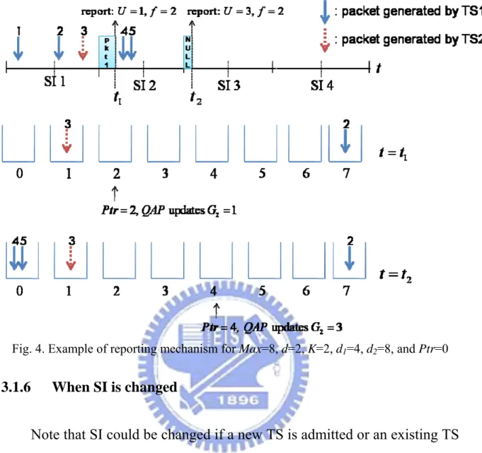
n (n≥1) SI, QAP changes Gf to U or does nothing if U =0. Figure 4 illustrates an example for Max=8, K =2,
2
d = , d1 =6, d2 =8, and Ptr=0. For this example, we have h=d2/d =4.
Initially, the partition list maintained in QAP satisfies Gi =0, 1≤ ≤i 4.
Assume that the TXOP allocated to QSTAp in the first SI is zero. Assume further that during the first SI, TS 1 generates one packet in each sub-interval and TS 2 generates one packet in the second sub-interval. If the TXOP allocated to QSTAp in the second SI is only enough to transmit a packet, then the reported value is U =1 and f =2, as shown in the middle
part of Figure 4. Note that Ptr is 2 at the beginning of the second SI.
Upon receiving the reported values, QAP updates G2 =1. Assume that the
TXOP allocated to QSTAp in the third SI is zero and, moreover, in the second SI, TS 1 generates two packets in the first sub-interval and zero packet in the second sub-interval and TS 2 does not generate any packet. As a result, as illustrated in the bottom part of Fig. 4, the value reported by
p
QSTA in the third SI is U =3 (which consists of one packet generated by
TS 2 in the first SI and two packets generated by TS 1 in the second SI) and
2
Chapter 3. Our Proposed Scheme
Fig. 4. Example of reporting mechanism for Max=8, d=2, K=2, d1=4, d2=8, and Ptr=0
3.1.6 When SI is changed
Note that SI could be changed if a new TS is admitted or an existing TS is finished. Consider now the situation when SI is changed. Assume that
d is changed to d'. Since all Max queues are in use, there is virtually no
impact on STA operation. The only work is to replace d with d'. As
for QAP, it needs to compute the new values of the partition list for each QSTA. Consider QSTAp and let G′i, 1≤ ≤i bK / 'd , be the new partition list maintained for QSTAp. Let z be the least common multiple of { , }h s such that z=ch=c s' , where s=bK / 'd . QAP computes gi+ −(j 1)c =Gj/c for
Chapter 3. Our Proposed Scheme
1 i c≤ ≤ and 1 j h≤ ≤ . The new G′i is then obtained as
' ( 1) ' 1 c i j i c j G g + − = ′ =
∑
, 1 i s≤ ≤ .Figure 5 shows an example of splitting the partition list. Initially, the partition list has three parts, i.e.: h=3. When a new TS is admitted, the SI is changed and the partition list is split into four parts in this example, i.e. s=4. How does QAP achieve this goal? QAP first calculate the values z=12, c=4 and c’=3. Each part of the original partition list first split into four parts, and every three parts merge into one part. Therefore, the new partition list has four parts and QAP allocates TXOP to each QSTA according to the new splitting partition list.
Chapter 3. Our Proposed Scheme
3.1.7 TXOP allocation to each QSTA
The TXOP allocation problem in our proposed SPRO-HCCA scheme is the same as that in the original PRO-HCCA scheme except that TXOPs are allocated to QSTAs instead of individual TSs. That is, the same classical fractional Knapsack problem is solved. However, the variable ti j, represents the transmission time allocated to data belonging to partition
,
i j
PL of QSTAi . Because of per-STA granularity, the computational
complexity of the proposed SPRO-HCCA scheme can be much smaller than that of the PRO-HCCA scheme if M is much larger than N. Besides, QAP needs to maintain only one partition list for each QSTA even if there are multiple TSs attached to the QSTA.
, , 1 1 , 1 1 , , maximize s.t. (6) 0 ( / ), 1, 2,..., ; 1, 2,...,
The TXOP allocated for is
N h i j i j i j N h i j avail i j i j i j k U t t T t PL R X i N j h QSTA TX = = = = ≤ ≤ ≤ + = =
∑∑
∑∑
, 1, 2, , (7) h k kj j OP =∑
t k = ⋅⋅⋅ NChapter 3. Our Proposed Scheme
3.2 Reducing Overhead SPRO-HCCA
3.2.1 Reducing the polling overhead
While maintaining the advantage of reporting, it is possible to reduce polling overhead of a QSTA if every TS attached to it has a delay bound
greater than or equal to four SIs. Consider QSTAp and let qp =⎣⎢b1/(2∗d)⎥⎦.
To reduce overhead, QAP can poll QSTAp once every qp SIs. For example, assume that SI =SIm and b1=4. For this example, QSTAp is polled once every two SIs. We call qp∗SI = qp∗ ∗d SIm the polling period of QSTAp. The idea can be applied to all QSTAs. Let qi∗SI,
1 i N≤ ≤ , denote the polling period of QSTAi. That is, QSTAi is polled by QAP once every qi SIs. As a result, different QSTAs may have different polling periods. The operations of QSTAi and QAP with respect to QSTAi are the same as those described in the last section as long as the polling period qi∗SI is treated as SI.
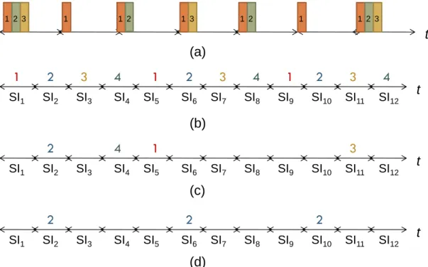
Figure 6 shows the different polling period of different QSTAs. In this example, there are three QSTAs, and polling period are SI, 2SI, and 3SI. The polling list period maintain by QAP is LCM(1,2,3)=6.
Chapter 3. Our Proposed Scheme t 1 1 12 3 1 1 2 3 2 1 1 2 3
Fig. 6. Example of different polling period of different QSTAs
3.2.1 Reducing the Partition List
Clearly, the partition list is still a source of complexity. One way to simplify the partition list as follows. Consider QSTAp. It always reports
the value 1 0 ( p ) / p q d Ptr q d j j U Q R ∗ − + ∗ + =
=
∑
to QAP. The partition list maintained byQAP for QSTAp has only two elements, i.e., Gp,1 =U and
,2 1 ( ) / K p i p i G e q SI R =
=
∑
∗ ∗ . Note that Gp,2 is the average transmission time of traffic arrivals to QSTAp in one polling period and is constant unless the TSs attached to QSTAp are changed. The same idea can be applied to all QSTAs. Consequently, there are only two elements in the partition list of every QSTA.3.2.2 Find the service start point
Since a QSTA could be polled once every several SIs, we need to decide how the QSTAs are polled. Define ALi =Gi,2, 1 i N≤ ≤ , as the
Chapter 3. Our Proposed Scheme
average load in transmission time offered by QSTAi in one polling period. Let PN =LCM q q( , ,...,1 2 qN) be the least common multiple of { , ,..,q q1 2 qN}. Time is divided into frames so that each frame consists of PN SIs. The SIs in a frame are numbered from 1 to PN. QAP maintains a polling list for each SI. It is clear that the polling lists are periodic with period PN and, therefore, the total number of polling lists maintained by QAP isPN. Note that the polling lists can be efficiently represented as a binary tree if
i
q =2ki
m
SI
∗ for all i, 1 i M≤ ≤ , where ki is a non-negative integer.
The polling lists are constructed as follows. To add the first QSTA
to the polling system, QAP decides SI =SImax,1, sets P1=1, and puts QSTA1
to the polling list for each SI. Assume that the polling lists are constructed for the existing N QSTAs and a new QSTA, i.e., QSTAN+1, is to be added to the system. Let TLi be the total average load offered by the QSTAs in the polling list of SI i. Assume that DN+1 does not change SI. The procedure to add QSTAN+1 to the polling system is as follows. QAP first computes PN+1 =LCM P q( ,N N+1) . Then it determines lj =
{
1}
1 1 0 (max/ ) 1 N N N j k q k P+ q + TL+ ∗ +≤ ≤ − for 1≤ ≤j qN+1 . After that, QAP finds i =
{ }
1 1 arg min N j j q l +Chapter 3. Our Proposed Scheme
k, 0≤ ≤k PN+1/qN+1−1. If DN+1 causes change of SI, then the new SI is
smaller than the original value. In this case, the construction procedure is performed for QSTA1, QSTA2, ..., and QSTAN+1 one by one with the new SI. Obviously, a similar procedure can be performed to update the polling lists if qk is changed for some k, 1 k≤ ≤N, due to change of TSs attached to
k
QSTA .
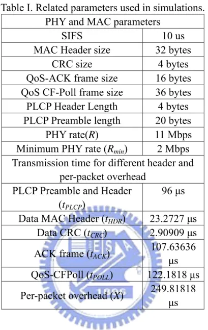
Figure.7. shows the example of adding a new QSTA and updating the polling list maintained by QAP. In Figure.7 (a), there are existing three QSTAs with polling periods SI, 2SI, and 3SI and QAP maintains a polling list with period 6SI. A new QSTA4 with polling period 4SI is added to the
system. In Fig.7 (b), QAP first determines the new polling list period PN+1=12 and compute the total traffic load of each polling list. In Fig.7 (c),
QAP picks up the maximum traffic load of each label, and determines the service start point that is the minimum traffic load we pick up. In this example, we pick up label 2 in Fig. 7(d), and the new QSTA is polled according the new updating polling list.
Chapter 3. Our Proposed Scheme t 1 1 1 2 3 1 1 2 3 2 1 1 2 3 1 2 3 t 4 SI2 SI1 SI3 SI4 SI5 SI6 SI7 SI8 SI9 SI10 SI11 SI12 2 2 2 t SI2 SI1 SI3 SI4 SI5 SI6 SI7 SI8 SI9 SI10 SI11 SI12 1 2 3 1 2 3 1 2 3 t 4 4 4 SI2 SI1 SI3 SI4 SI5 SI6 SI7 SI8 SI9 SI10 SI11 SI12 (a) (b) (c) (d)
Chapter 4. Experimental Result
Chapter 4.
Experimental Result
The PHY and MAC parameters and all related information used in simulations are shown in Table I. Note that the sizes of QoS-ACK and QoS-Poll in the table only include the sizes of MAC header and CRC overhead. We assume that the minimum physical rate is 2Mbps and tPLCP is reduced to 96 μs. It is assumed that SIm =10ms. Two types of TSs,
with characteristics and QoS requirements shown in Table II, are considered in simulations. Type I and Type II TSs are lecture room cam and interactive video, respectively. We assume that 90% of the bandwidth is used by HCCA, i.e., ρhcca=0.9.
Chapter 4. Experimental Result
Table I. Related parameters used in simulations. PHY and MAC parameters
SIFS 10 us
MAC Header size 32 bytes CRC size 4 bytes QoS-ACK frame size 16 bytes QoS CF-Poll frame size 36 bytes PLCP Header Length 4 bytes PLCP Preamble length 20 bytes
PHY rate(R) 11 Mbps Minimum PHY rate (Rmin) 2 Mbps
Transmission time for different header and per-packet overhead
PLCP Preamble and Header (tPLCP)
96 μs Data MAC Header (tHDR) 23.2727 μs
Data CRC (tCRC) 2.90909 μs
ACK frame (tACK)
107.63636 μs
QoS-CFPoll (tPOLL) 122.1818 μs
Per-packet overhead (X) 249.81818 μs
Table II. TSPECs for two different types of traffic flows. Traffic characteristics and
QoS requirements Type I Type II Maximum Service Interval 20 ms 40 ms
Delay Bound 40 ms 80 ms Mean Data Rate 42 Kbps 246 Kbps Nominal MSDU size 211 bytes 1232 bytes Scheduled Service Interval 20 ms
Chapter 4. Experimental Result
In the first experiment, we compare the performances of the sample scheduler, the PRO-HCCA scheduler, the SPRO-HCCA scheduler, and the reduced-overhead SPRO-HCCA (RO-SPRO-HCCA) scheduler with real traces [17]. There are three QSTAs. QSTA1, QSTA2, and QSTA3 that are
attached with two Type I TSs, one Type I TS and another Type II TS, and two Type II TSs, respectively. As a result, the scheduled SI is set to 20 ms = 2SIm. The polling order is QSTA1, then QSTA2, followed by QSTA3.
In the PRO-HCCA scheme, for the two TSs attached to QSTA2, the Type I
TS is polled before the Type II TS. Because of the 80 ms delay bound, Type II TSs attached to QSTA3 are polled once every two SIs in the
RO-SPRO-HCCA scheme.
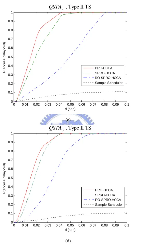
Figs. 8(a)-8(d) show the cumulative distribution functions (CDFs) of delay for TSs attached to various QSTAs. Note that, as illustrated in Fig. 8(a), the RO-SPRO-HCCA scheme is the same as the SPRO-HCCA scheme for the TSs attached to QSTA1. One can see in Fig. 8(a) that
packets of TSs attached to QSTA1 experience roughly the same delay under
the SPRO-HCCA scheme and the PRO-HCCA scheme. The curves shown in Fig. 8(b) reveal that packets of Type I TS attached to QSTA2
experience smaller delay under the SPRO-HCCA scheme than the PRO-HCCA scheme. The reason is that packets of Type I TS have smaller delay bound than packets of Type II TS and, therefore, under the SPRO-HCCA scheme, may use the bandwidth allocated to packets of Type
Chapter 4. Experimental Result
II TS that can be kept for more than two SIs. Because of this, packets of the Type II TS experience larger delay under the SPRO-HCCA scheme than the PRO-HCCA scheme, as can be seen in Fig. 8(c). Note that the RO-SPRO-HCCA scheme is different from the SPRO-HCCA scheme for
2
QSTA . There are four entries for the partition list maintained for QSTA2
under the SPRO-HCCA scheme. However, under the RO-SPRO-HCCA scheme, there are only two entries for the partition list maintained for
2
QSTA and only the data that will violate their delay bounds if not served in
the next SI are reported to QAP. Packets experience more delay under the RO-SPRO-HCCA scheme than under the SPRO-HCCA scheme and the PRO-HCCA scheme. However, all packets meet their delay bounds. The sample scheduler obviously cannot meet QoS requirements. Although the PRO-HCCA, SPRO-HCCA, and RO-SPRO-HCCA schedulers meet QoS requirements, their ratios of overhead transmission time to total transmission time are different. They are 34.92%, 31.40%, and 29.51% for the PRO-HCCA, SPRO-HCCA, and RO-SPRO-HCCA schemes, respectively.
Chapter 4. Experimental Result 0 0.01 0.02 0.03 0.04 0.05 0.06 0.07 0.08 0.09 0.1 0 0.1 0.2 0.3 0.4 0.5 0.6 0.7 0.8 0.9 1 d (sec) P (ac c es s del ay < = d) PRO-HCCA SPRO-HCCA RO-SPRO-HCCA Sample Scheduler 1 , Type I TS QSTA (a) 0 0.01 0.02 0.03 0.04 0.05 0.06 0.07 0.08 0.09 0.1 0 0.1 0.2 0.3 0.4 0.5 0.6 0.7 0.8 0.9 1 d (sec) P (ac c es s del ay < = d) PRO-HCCA SPRO-HCCA RO-SPRO-HCCA Sample Scheduler 2 , Type I TS QSTA (b)
Chapter 4. Experimental Result 0 0.01 0.02 0.03 0.04 0.05 0.06 0.07 0.08 0.09 0.1 0 0.1 0.2 0.3 0.4 0.5 0.6 0.7 0.8 0.9 1 d (sec) P (a c c e ss d e la y< = d ) PRO-HCCA SPRO-HCCA RO-SPRO-HCCA Sample Scheduler 2 , Type II TS QSTA (c) 0 0.01 0.02 0.03 0.04 0.05 0.06 0.07 0.08 0.09 0.1 0 0.1 0.2 0.3 0.4 0.5 0.6 0.7 0.8 0.9 1 d (sec) P (ac c es s del ay < = d) PRO-HCCA SPRO-HCCA RO-SPRO-HCCA Sample Scheduler 3 , Type II TS QSTA (d)
Fig. 8. Performance comparison of various schedulers for three different QSTAs.
Chapter 4. Experimental Result
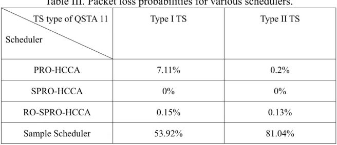
In the second experiment, we assume that there are one Type I TS and one Type II TS attached to each QSTA. Simulations are performed to determine the maximum number of QSTAs N that can be supported
without violating delay bound requirements under the SPRO-HCCA scheme. The result is N =11. Therefore, we simulate a system which
consists of 11 QSTAs under various scheduling schemes. QSTAs are polled one by one. In the PRO-HCCA scheme, Type I TS is polled before Type II TS attached to the same QSTA. Note that, similar to the situation of QSTA2 in the first experiment, the RO-SPRO-HCCA scheme is different
from the SPRO-HCCA scheme for this experiment. Figs. 9(a) and 9(b) show, respectively, the CDFs of delay for packets of Type I TS and Type II TS attached to the eleventh QSTA. As one can see from the figures, the SPRO-HCCA scheme outperforms the PRO-HCCA scheme for both types of TSs. The phenomenon we observed for QSTA2 in the first experiment,
i.e., the bandwidth allocated to less urgent packets of Type II TS could be used by packets of Type I TS, does not appear in the second experiment. The reason is that almost all bandwidth are allocated to the most urgent packets that will be dropped if not served in the next SI. Some packets violate their delay bounds and are lost under the PRO-HCCA scheme because it suffers from higher overhead than the SPRO-HCCA scheme. The packet loss probabilities due to violation of delay bounds are summarized in Table III. The low packet loss probabilities make the RO-SPRO-HCCA an attractive scheme for real systems.
Chapter 4. Experimental Result 0 0.01 0.02 0.03 0.04 0.05 0.06 0.07 0.08 0.09 0.1 0 0.1 0.2 0.3 0.4 0.5 0.6 0.7 0.8 0.9 1 d (sec) P (a c c e ss d e la y< = d ) PRO-HCCA SPRO-HCCA RO-SPRO-HCCA Sample Scheduler 11 , Type I TS QSTA (a) 0 0.01 0.02 0.03 0.04 0.05 0.06 0.07 0.08 0.09 0.1 0 0.1 0.2 0.3 0.4 0.5 0.6 0.7 0.8 0.9 1 d (sec) P (a c c es s del ay < = d) PRO-HCCA SPRO-HCCA RO-SPRO-HCCA Sample Scheduler 11 , Type II TS QSTA (b)
Fig. 9. Performance comparison of various schedulers for eleven identical QSTAs.
Chapter 4. Experimental Result
Table III. Packet loss probabilities for various schedulers.
TS type of QSTA 11 Scheduler Type I TS Type II TS PRO-HCCA 7.11% 0.2% SPRO-HCCA 0% 0% RO-SPRO-HCCA 0.15% 0.13% Sample Scheduler 53.92% 81.04%
Chapter 5. Conclusion
Chapter 5.
Conclusion
We have presented in this paper a per-QSTA based scalable TXOP allocation scheme for HCCA to guarantee QoS for VBR traffic in WLANs. The scheme is modified to allow different polling periods for different traffic streams. Computer simulations with real traces show that our proposed schemes meet QoS requirements. Besides, according to simulation results, our proposed schemes utilize bandwidth more efficiently than the sample scheduler and the PRO-HCCA scheduler. An advantage of the proposed schemes is that they do not require traffic models. It suffices to know the mean arrival rate of each traffic stream. Simplicity and robustness make the proposed schemes good candidates of the TXOP allocation scheme for HCCA to guarantee QoS for variable bit rate traffic streams.
Bibliography
Bibliography
[1] IEEE 802.11 WG: IEEE Standard 802.11-1999, Part 11: Wireless LAN MAC and Physical Layer Specifications. Reference number ISO/IEC 8802-11: 1999(E), 1999.
[2] IEEE Std. 802.11e-2005, Part 11: Wireless LAN medium access control and physical layer specifications Amendment 8: medium access control (MAC) quality of service enhancements, Nov. 2005.
[3] S. Mangold, S. Choi, G. R. Hiertz, et. All, “Analysis of IEEE 802.11e for QoS support in Wireless LANs,” IEEE Wireless Commun., vol. 10, no. 6, pp. 40-50, Dec. 2003.
[4] P. Ansel, Q. Ni, and T. Turletti, “FHCF: A fair scheduling scheme for IEEE 802.11e WLAN,” INRIA research report, no. 4883, Jul. 2003. [5] Y. Higuchi, A. Foronda, C. Ohta, M. Yoshimoto and Y. Okada, “Delay
guarantee and service interval optimization for HCCA in IEEE 802.11e WLANs,” in Proc. IEEE WCNC 2007.
[6] A. Annese, G. Boggia, P. Camarda, L. A. Grieco, and S. Mascolo, “Providing delay guarantees in IEEE 802.11e networks,” in Proc. WWIC 2005.
[7] W. F. Fan, D. Y. Gao, D. H. K. Tsang and B. Bensaou, “Admission Control for variable bit rate traffic in IEEE 802.11e WLANs,” in Proc. IEEE LANMAN 2004.
[8] Y. W. Huang, T. H. Lee and J. R. Hsieh, “Gaussian approximation based admission control for variable bit rate traffic in IEEE 802.11e WLANs,” in Proc. IEEE WCNC 2007.
Bibliography
[9] T. H. Lee and Y. W. Huang, “Effective transmission opportunity allocation scheme for real-time variable bit rate traffic flows with different delay bounds,” IET Commun., vol. 2, no. 4, pp. 598-608, 2008.
[10] M. M. Rashid, E. Hossain, V. K. Bhargava, “HCCA scheduler design for guaranteed QoS in IEEE 802.11e based WLANs,” in Proc. IEEE WCNC 2007.
[11] M. M. Rashid, E. Hossain, V. K. Bhargava, “Controlled channel access scheduling for guaranteed QoS in 802.11e-based WLANs,” IEEE Trans. Wireless Communications, vol. 7, no. 4, Apr. 2008.
[12] Q. Zhao and D. Tsang, “An equal-spacing-based design for QoS guarantee in IEEE 802.11e HCCA wireless networks,” IEEE Trans. Mobile Computing, vol. 7, no. 11, Nov. 2008.
[13] H. Fattah and C. Leung, “An overview of scheduling algorithm in wireless multimedia networks,” IEEE Wireless Commun., vol. 9, no. 5, pp. 76-83, Oct. 2002.
[14] B. Farhang-Boroujeny, Adaptive Filters: Theory and Applications. New York: Wiley, 1998.
[15] T. Cormen, C. Leisorson, R. Rivest, and C. Stein, Introduction to Algorithms, Second Edition. Cambridge, MA: MIT Press, 2001.
[16] J. Choe and N. B. Shroff, “A central limit theorem based approach for analyzing queue behavior in high-speed networks,” IEEE/ACM Trans. Networking, vol. 6, no. 5, pp. 659-671, Oct. 1998.
[17] MPEG-4 and H.263 video traces for network performance evaluation,
http://www.tkn..tu-berlin.de/research/trace/trace.html, Oct. 2006.
Bibliography
Intrusion Detection System Using PCA and BNN,” in Proc. Information and Telecommunication Technologies, 6th Asia-Pacific Symposium, p.p. 356-359, 10-10 Nov. 2005