平行化路徑式KNN查詢演算法運用於無線感測器網路

(1)

國

立

交

通

大

學

資訊科學與工程研究所

碩

士

論

文

平行化路徑式ＫＮＮ查詢演算法運用於無

線

感

測

器

網

路

Parallel Itinerary-based KNN Query Processing in

Wireless Sensor Networks

研究生：傅道揚

指導教授：彭文志教授

(2)

96 碩

士

論

文

平行化路徑式 KNN 查詢演算法運用於無線感測器網路

96 碩

士

論

文

96 碩

士

論

文

96 碩

士

論

文

96 碩

士

論

文

平行化路徑式 KNN 查詢演算法運用於無線感測器網路交通大學交通大學交通大學交通大學交通大學資訊科學與工程研究所資訊學院資訊科學與工程研究所資訊學院資訊科學與工程研究所資訊學院資訊科學與工程研究所資訊學院資訊科學與工程研究所資訊學院

傅道揚

9555514

傅道揚

9555514

傅道揚

9555514

傅道揚

9555514

傅道揚

9555514

(3)

平行化路行式 KNN 查詢演算法運用於無線感測器網路

Parallel Itinerary-based KNN Query Processing in

Wireless Sensor Networks

研究生：傅道揚 Student：Tao-Yang Fu

指導教授：彭文志 Advisor：Wen-Chih Peng

國立交通大學

資訊科學與工程研究所

碩士論文

A Thesis

Submitted to Institute of Computer Science and Engineering College of Computer Science

National Chiao Tung University in partial Fulfillment of the Requirements

for the Degree of Master

in

Computer Science

June 2008

Hsinchu, Taiwan, Republic of China

(4)

謫要在無線感測器網路中，用來得到給定的限制條件下的感測資料的空間式的查詢，可以運用在許多應用中，例如：環境監測、軍事監視等。一種典型的空間式查詢，KNN 查詢，便是給定一空間上的查詢位置，以及欲收集的資料個數 K 值，來收集空間中感測到的資料。近期的研究中，一種路徑式的 KNN 查詢演算法被發展出來，乃沿著預先計算好的路徑來作資料的收集的演算法，被研究出較其他演算法，可以達到較好的電力效率。但是，路徑式 KNN 演算法中，如何設計以及計算出路徑，便是此種演算法的一大挑戰。在此篇論文中，我們提出一種新的路徑式 KNN 查詢演算法，叫作 PCIKNN，根據使用者不同的目的，例如：最佳化查詢時間、最佳化電力消耗，來計算出查詢路徑。PCIKNN 的效能，在數學上以及實驗上被證明較目前其他路徑式 KNN 演算法，擁有較好的效能，在於查詢精確度、查詢時間以及電力消耗等。 i

(5)

Abstract

Spatial queries for extracting data from wireless sensor networks are important for many ap-plications, such as environmental monitoring and military surveillance. One such query is K Nearest Neighbor (KNN) query that facilitates sampling of monitored sensor data in cor-respondence with a given query location. Recently, itinerary-based KNN query processing techniques, that propagate queries and collect data along a pre-determined itinerary, have been developed concurrently [27][30]. These research works demonstrate that itinerary-based KNN query processing algorithms are able to achieve better energy efficiency than other existing algorithms. However, how to derive itineraries based on different performance re-quirements remains a challenging problem. In this paper, we propose a new itinerary-based KNN query processing technique, called PCIKNN, that derives different itineraries aiming at optimizing two performance criteria, response latency and energy consumption. The perfor-mance of PCIKNN is analyzed mathematically and evaluated through extensive experiments. Experimental results show that PCIKNN has better performance, such as accuracy, energy consumption and query latency, and has scalability than the state-of-the-art.

(6)

致謝本篇論文能夠順利的完成，要感謝的人非常的多。首先，是我的指導教授，彭文志教授，在碩士兩年的過程，我學習了很多研究的精神和方式，論文撰寫的技巧，有他的教導和協助，讓我能從更多元、更完整的角度來作研究以及完成此篇論文。其次，是一起合作的美國賓州州立大學的李旺謙教授，因為在碩一時因緣際會的合作，才有此篇論文方向的確定，藉由不斷的合作，來讓此篇論文更加的完整。再來是我的家人，家人對我的支持，是我不斷前進的動力，也讓我能無後顧之憂的來完成我的學業。最後，要謝謝實驗室中的所有夥伴，有學長們的督促和鼓勵，同學們的陪伴和討論，讓我的碩士生活非常豐富及充實，也從你們身上看到了對人生的衝勁，並且留下了美好的回憶。 iii

(7)

List of Figures

1.1 Overview of itinerary-based KNN query processing. . . 2

2.1 Itinerary-based query propagation. . . 5

2.2 Parallel concentric itineraries in PCIKNN. . . 7

3.1 Itinerary structures in IKNN and DIKNN. . . 10

3.2 Analytical latency and energy consumption with the number of sectors varied. 10 3.3 Information statistics in routing path. . . 14

3.4 Models validation. . . 17

4.1 Estimating coverage areas of routing. . . 18

4.2 Intersection covered area with various node distances. . . 19

5.1 Updating KNN boundary dynamically. . . 22

6.1 Impact of network density. . . 28

6.2 Impact of K. . . 29

6.3 Impact of node mobility. . . 30

6.4 Impact of node failure rate. . . 32

6.5 KNN boundary estimation of DIKNN and PCIKNN. . . 33

(10)

List of Tables

(11)

Chapter 1 Introduction

Recent advances in micro-sensing MEMS and wireless communication technologies have mo-tivated the development of wireless sensor networks (WSN). A WSN which consists of a large number of sensor nodes capable of sensing, computing, and communications, can be used in a variety of applications such as border detection systems, ecological monitoring systems, and intelligent transportation systems. Generally speaking, WSNs are deployed over a wide geographical area to facilitate long-term monitoring and data collection tasks. As sensing readings are geographically distributed, spatial queries that aim at extracting sensing data from sensor nodes located in certain areas of interests are essential to many WSN applications [13][18]. In this paper, we focus on the processing of K nearest neighbors (KNN) query, which facilitates data sampling of the sensors located in a geographical proximity via specification of a query point q and a sample size K. Using a KNN query, one could obtain sensor data (e.g., environmental measurements) near a query location of interests. A KNN query processing is a classical spatial query in a centralized databases and has attracted many research efforts to improve the performance of KNN query processing [19][22][8][23][4]. However, traditional KNN processing techniques are infeasible for wireless sensor networks in that a centralized database should be built to periodically collect sensing data from large-scale sensor networks, which incurs higher energy consumption and long latency.

To overcome the issues mentioned above, in-network processing techniques for KNN queries have been developed [5][2][24][25][30][27][28]. In these papers, a KNN query is submitted to the network via any sensor node (referred to as the source node) and propagated to the sensor nodes qualified by specified predicates. As a result, sensor data from these nodes are collected and returned to the source node. Existing in-network KNN query processing

(12)

home node query point q

source node

initial KNN boundary

updating KNN boundary

1. Query routing phase

2. KNN boundary estimation phase 3. Query dissemination phase

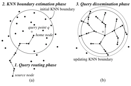
Figure 1.1: Overview of itinerary-based KNN query processing.

[20][1] or spanning trees [14][15] in WSN) for query propagation and processing [5][24][25]. Maintenance of those network infrastructures is a major issue of this type of query processing techniques. In particular, maintaining infrastructures incurs excessive communications when sensors have the mobility capability [3][7]. On the other hand, the latter does not rely on any pre-established network infrastructure to process queries. Recently, two infrastructure-free KNN query processing techniques have been developed [30][27][28]. The main idea of these infrastructure-free KNN query processing is that a KNN query is propagated along well-designed itineraries and data is collected while the KNN query performs itinerary traversals.

Without loss of generality, an itinerary-based KNN query processing algorithm typically consists of three phases: i) routing phase; ii) KNN boundary estimation phase; iii) query dissemination phase. The execution example of itinerary-based KNN query processing is shown in Figure 1.1. Explicitly, when a KNN query Q is issued at a source node, the query Q that specifies the query point q and the sample size K is routed to the sensor node nearest to the query point q (referred the home node) by geo-routing protocols (e.g., GPSR [9], PSGR [26] and other geo-routing protocols [10][11]). Then, in the KNN boundary estimation phase, the home node will estimate the initial KNN boundary (e.g., the solid boundary shown in Figure 1.1(a)), where KNN boundary is likely to contain K sensor nodes. After estimating the initial KNN boundary, in the query dissemination phase (shown in Figure 1.1(b)), the home node propagates the query to each node within the KNN boundary. A KNN query is propagated along well-designed itineraries, while partial query results are aggregated at the same time. It is shown in [30][27][28], by avoiding the maintenance of a network infrastructure, itinerary-based KNN query processing techniques outperform existing infrastructure-based

(13)

KNN approaches.

Clearly, the performance (such as the query latency and the energy consumption) of itinerary-based KNN query processing techniques is dependent on the design of itinerary structures. With a long itinerary, long processing latency and high energy consumption are expected due to the long itinerary traversal of a KNN query. Thus, itinerary planning is a vitally important design issue for itinerary-based KNN query processing. Prior works in [30][27][28] develop several itinerary structures. However, the proposed itineraries are not op-timized in terms of the energy consumption and the query latency. In this paper, we propose a new itinerary-based KNN query processing technique that derives parallel itineraries aim-ing at optimizaim-ing two performance criteria, the query latency and the energy consumption. Specifically, we propose a Parallel Concentric-circle Itinerary-based KNN query processing (thus named as PCIKNN ). In this paper, PCIKNN is designed to allow a KNN query propa-gated in multiple concurrent itineraries and the number of concurrent itineraries (referred to as KNN threads for short) is maximal. Intuitively, with a larger number of concurrent KNN threads propagated, both the query latency and the energy consumption are significantly re-duced. Furthermore, analytical models for the query latency and the energy consumption of PCIKNN are derived. By optimizing the latency and the energy consumptions, PCIKNN derives itineraries with two modes (i.e., min latency mode and min energy mode), specifi-cally tailored to minimize the response latency or the energy consumption, respectively. For itinerary-based KNN query processing techniques, an important issue is to estimate a search boundary covered by itineraries. Thus, by exploring regression techniques, we proposed a boundary estimation method to accurately determine the search boundary. In addition, to improve the query accuracy, we develop several mechanisms to dynamically adjust the search boundary. The performance of PCIKNN is analyzed mathematically and evaluated through extensive experimentation based on simulation. Experimental results show that PCIKNN has better performance and scalability than the state-of-the-art.

The rest of the paper is organized as follows. Preliminaries, including the problem defi-nition and basic ideas of existing itinerary-based KNN query processing is introduced. The design of our PCIKNN technique and analytic models for two optimization modes are de-scribed in Chapter 3. A KNN boundary estimation is presented in Chapter 4. Mechanisms for spatial irregularity are developed in Chapter 5. The performance of PCIKNN and other existing techniques is evaluated in Chapter 6. Finally, Chapter 7 concludes this paper.

(14)

Chapter 2 Preliminaries

In this chapter, some assumptions and KNN problem definition is presented. Then, the problem addressed in this paper is described.

2.1 Assumptions

We assume that sensor nodes in wireless sensor networks are randomly distributed in a two-dimensional space. Each sensor is location-aware via GPS [17] or other localization techniques. By periodically inter-exchanging information among sensor nodes nearby, a sensor node is able to maintain its own neighboring information. Moreover, we assume that the sensed data are stored locally on the sensor nodes. KNN queries can be issued at any sensor node (called source node), which is the starting node for in-network query processing. The source node is also responsible for reporting the query result after query processing. As mentioned before, KNN query processing provides a way to sample the data from sensor nodes located in the proximity of a given query location. We now define the KNN query in wireless sensor networks as follows:

Definition: (K Nearest Neighbor query). Given a set of sensor nodes M and a geographical

location (denoted as a query point q), find a subset M′ _{of k nodes (M}′ _{⊆ M, |M}′_{| = K)}

such that ∀n1 ∈ M′ and ∀n2 ∈ M − M′, dist(n1, q) ≤ dist(n2, q), where dist represents the

Euclidean distance function.

Generally speaking, the exact result set of KNN should contain the K nearest neighbor nodes of q. However, due to the mobility nodes and the network spatial irregularity, prior works only provide approximate KNN query result and the query result accuracy is defined by the percentage ratio of the correct KNNs returned. In itinerary-based KNN query processing techniques, the main phase is the query dissemination phase. Thus, in the following, we

(15)

describe the query dissemination phase in details.

2.2 Query Dissemination Phase in Itinerary-based KNN

Query Processing

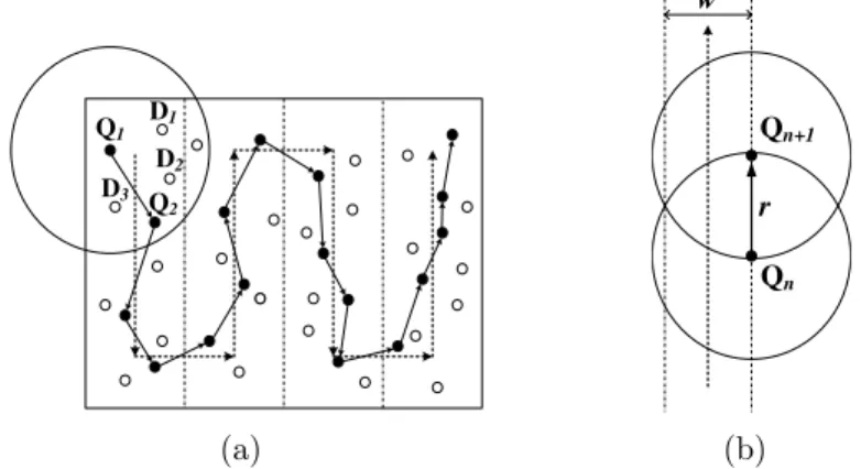
Q1 Q2 D3 D2 D1 (a) w Qn Qn+1 r (b)

Figure 2.1: Itinerary-based query propagation.

Query dissemination is a critical issue for itinerary-based KNN query processing tech-niques. The detailed steps of itinerary-based query dissemination are illustrated in Fig-ure 2.1(a), where the dotted line is a well-designed itinerary. As shown in the figFig-ure, sensors are categorized into Q-node (marked as black nodes) and D-node (marked as white nodes). Upon receiving a query, a Q-node broadcasts a probe message including the query Q and the itinerary information to its neighbors. Each neighbor node (i.e., D-node) receives the probe message and then sends its sensed data to the Q-node. After collecting data from D-nodes nearby, the Q-node finds the next Q-node along the itinerary and forwards the current query result to the next Q-node. The next Q-node is determined by exploring the maximum progress heuristic in that the next Q-node with the farthest distance to the current Q-node along the

proceeding direction of the itinerary is selected. The width of the itineraries w is set to √3

2 r,

where r is the transmission radius of a sensor node, for full coverage shown in Figure 2.1(b). Interesting readers are referred to [16] [29] for detailed implementation of itinerary-based query dissemination. Finally, the last Q-node forwards the aggregated query result to the source node, where the KNN query is issued.

(16)

2.3 Overview of PCIKNN

In this paper, we propose a new itinerary-based query processing algorithm based on optimized parallel concentric-circle itineraries, named as PCIKNN. Same as in prior works in [30][27], PCIKNN also has three phases: the routing phase, the KNN boundary estimation phase and the query dissemination phase. In addition, to improve the query accuracy of KNN query, PCIKNN has several mechanisms to improve the accuracy of KNN query results. Explicitly, the estimated KNN boundary could be dynamically updated while the query is propagated within the KNN boundary. Moreover, the KNN result collection should be guaranteed based on information exchanging within adjacency itineraries. Finally, aggregated query results are sent back to the source node.

As mentioned before, itinerary structures have a great impact on the performance of itinerary-based KNN query processing techniques. Long itineraries may incur long latency and heavy energy consumption, because the query propagation and data collection are per-formed along the itineraries. A query may have a long journey and have to carry more collected data on long itineraries, thereby increasing both the latency and the energy consumption. In addition to the length and the number of itineraries, the number of concurrent KNN query threads propagated also have an impact on performance of itinerary-based KNN query pro-cessing techniques. Clearly, with a larger number of concurrent threads propagated along itineraries, the latency of KNN query processing may be improved. However, prior works explore multiple itineraries by fixing the number of concurrent KNN query threads to the number of itineraries. Thus, in PCIKNN, we aim at designing itineraries that allow more con-current KNN query threads to be propagated. Since the routing phase of PCIKNN is the same as in [30][27][28], in the following sections, we will describe the itinerary structure designed in PCIKNN, the estimation method in the boundary estimation phase and the mechanisms for improving the accuracy of KNN results.

(17)

branch- peri- return-maximum search path KNN boundary S1 S4 S2 S3 w/2 w

(18)

Chapter 3 Itinerary Structures in PCIKNN

In this chapter, we first present the design of parallel concentric-circle itineraries in PCIKNN and then an analytical comparison of performances between PCIKNN and existing works are derived. Moreover, corresponding to the targeted performance criteria, i.e., the query latency and the energy consumption, we analytically derive the number of parallel itineraries to be employed in PCIKNN.

3.1 Parallel Concentric-Circle Itineraries

As pointed before, the number and structure of itineraries have an impact on performance of itinerary-based KNN query processing algorithms. Intuitively, a KNN query executed concur-rently through a large number of itineraries will incur small latency and energy consumptions. However, in reality, it’s not feasible to use an excessive number of itineraries due to that the packet collision problem [27][28]. Here, we first explore the design issue of parallel concentric-circle itineraries by assuming a boundary that contains K nearest sensor nodes to the query point is given. We will address the issue of estimating this KNN boundary later in Chapter 4. Given a query point q and an estimated KNN boundary, the area within the boundary

can be divided into multiple concentric-circle itineraries. Let Ci denote the ith circle with

a radius w × i, where w is the itinerary width, the distance between itineraries. Similar to

[30][27][28], w can be set as √₂3r, where r is the transmission range of a sensor node. In order

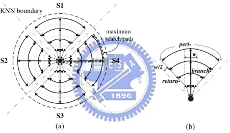
to propagate KNN query along concentric-circle itineraries, we partition the KNN boundary into multiple sectors. Figure 2.2(a) shows an example of concentric-circle itineraries, where the number of sectors is 4. For each sector, we have three types of itinerary segments: 1) a branch-segment, 2) a set of peri-segments, and 3) two return-segments. As shown in Figure 2.2(b), a branch segment is a straight line passed through concentric-circles with the itinerary width w

(19)

in each sector, two return-segments are the boundary lines among sectors with the itinerary

width w₂ and peri-segments are portions of concentric-circles between branch-segments and

return-segments. Obviously, there is no peri-segment in a concentric-circle if the regions of branch-segments and return-segments fully cover this concentric-circle. It can be seen that in Figure 2.2(b) the arrows indicate the directions of query propagations. With the segments of itineraries in PCIKNN, a KNN query is executed concurrently at these segments of itineraries and the KNN query propagated in these segments are referred to as KNN query threads. Note that the number of concurrent KNN query threads in PCIKNN is as maximal as possible.

In light of itinerary segments derived above, a KNN query is disseminated along these seg-ments of itineraries. A KNN query propagation starts from the home node and the KNN query is first propagated along with branch-segments in each sector. Along the branch-segment, a Q-node broadcasts a probe message and aggregates the partial results from D-nodes within the region width of w. Then, for each sector, when the KNN query reaches one of concentric-circles, two KNN query threads are forked to propagate along the two peri-segments, while the original KNN query continues to move along the branch-segment. To propagate a KNN query in two segments, the Q-node in the branch segment first finds two Q-nodes in peri-segments and evenly divide the partial query result collected to these two Q-nodes. Then, these two Q-nodes will start performing KNN query dissemination with peri-segments. When KNN queries propagating along peri-segments arrive the boundary lines of their sectors, KNN queries with data collected are returned back to the home node through return-segments. Because the home node receives all partial KNN query results, it is able to decide whether to continue KNN query propagation or not. This leads to more precise KNN query results in PCIKNN. The detailed mechanisms to improve the query accuracy is presented later. The above query dissemination repeats until the original KNN query reaches the outer concentric-circle. Hence, in PCIKNN, the number of the concurrent KNN threads is larger than prior works [30]DIKNN. It can be seen that by exploring parallel concentric-circles, the number of concurrent KNN query threads is maximized. Furthermore, due to the high parallelism of PCIKNN, PCIKNN achieves high performance in terms of the query latency and the energy consumption.

(20)

KNN boundary (a) IKNN S1 S2 S4 S3 KNN boundary (b) DIKNN

Figure 3.1: Itinerary structures in IKNN and DIKNN.

0 high

4 5 6 7 8 9 10 11 12

Estimated Latency

(evaluated by itinerary length)

Number of Sectors PCIKNN

DIKNN

(a) Latency analysis

0 high

4 5 6 7 8 9 10 11 12

Estimated Energy Consumption (evaluated by itinerary length)

Number of Sectors PCIKNN

DIKNN

(b) Energy analysis

(21)

Without loss of generality, we assume that sensor nodes are uniformly distributed in the monitored region. Moreover, the KNN boundary is known and in our illustrative example, the radius R of the KNN boundary is set to c×w. In other words, there are c concentric-circles in the KNN boundary. In addition, the number of sectors is set to S.

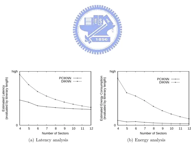
Number of concurrent query threads: Figure 3.1(a) shows the parallel IKNN algorithm proposed in [30]. As can be seen in Figure 3.1(a), since there are two itineraries, the number of concurrent query threads in IKNN is 2. For DIKNN and PCIKNN, the number of sectors directly affects the number of concurrent query threads. It can be seen that in Figure 3.1(b), only one itinerary is in a sector of DIKNN and hence the number of concurrent query threads in DIKNN is exactly the same with the number of sectors. In PCIKNN, for each sector, one could have one query thread along with a branch-segment, two query threads alone with peri-segments in each concentric circle. Therefore, the maximal number of concurrent KNN query threads is (2 × c + 1) × S. Assume that the number of sectors is set to 4 and the number of concentric-circles is 4. As such, we could have the number of concurrent query threads in DIKNN and PCIKNN as 4 and 36, respectively. Clearly, PCIKNN has the maximal number of query threads compared to IKNN and DIKINN.

As pointed out early, sensor nodes are uniformly distributed in the network and the width of itineraries for query propagation and data collection is w. Consequently, the query latency and the energy consumption are highly proportional to the length of itineraries. As such, for the analysis of the query latency and the energy consumption, the comparisons of DIKNN and PCIKNN are in terms of the length of itineraries. Note that since DIKNN outperforms IKNN, we only compare DIKNN and PCIKNN.

Query latency: The query latency is determined by the maximal length of itineraries in DIKNN and PCIKNN. Therefore, we derive the maximal length of itineraries shown as the dotted lines in Figure 3.1(b) and Figure 2.2(a) to represent the query latency (denoted as the analytical latency). As shown in Figure 3.1(b), it can be seen that the analytical query latency of DIKNN is the sum of the total lengths of concentric-circles in a sector and the length of a branch-segment. Hence, we have

analytical latencyDIKN N =P

R w

i=0(LengthCi) + Lengthbranch

, where the length of itinerary in the i th concentric-circle LengthCi = 2π(i×w)_S and the length

of branch-segment Lengthbranch = (c − 1₂) × w.

(22)

analytical latencyP CIKN N = Lengthperi+ Lengthbranch

, where the length of peri-segments Lengthperi= π×R_S in the maximal concentric-circle and the

length of a branch-segment Lengthbranch = (c − 1₂) × w. The result of the analytical latency

for DIKNN and PCIKNN with the number of sectors varied is shown in Figure 3.2(a). It can be seen in Figure 3.2(a) that the analytical latency in DIKNN and PCIKNN decreases when the number of S increases. This is due to that with a larger number of sectors, the smaller of the maximal length of itineraries in both DIKNN and PCIKNN. Moreover, the analytical latency of PCIKNN is smaller than that of DIKNN. As a result, PCIKNN is expected to have better latency performance than others.

Energy consumption: In itinerary-based KNN query processing techniques, the data

collected is carried along with the itineraries during the query propagation. Clearly, the energy consumption of DIKNN and PCIKNN could be evaluated by the amount of data carried. With a longer itinerary, the number of Q-nodes on the itinerary and the amount of data carried will be increased. Thus, the analytical energy consumption is estimated as analytical energy =

S ∗ analytical energys, where analytical energysis the energy consumption in one sector and

S is the number of sectors. Intuitively, the value of analytical energys can be derived by

integrating the length of itineraries and the amount of data carried. Denote the length of

itineraries in a sector as lengths. Since the amount of data carried is directly proportional

to the itinerary length, we could use a continuous function of itinerary lengths, denoted as Damount(∗), to model the energy consumption. Hence, we could have the following formula:

analytical energys =

Rlengths

x=0 Damount(x) × d(x) ∝ (itinerary length) 2

Therefore, the analytical energy could be a quadratic function of itinerary lengths in a sector. The analytical energy of DIKNN is formulated as the sum of the square of the total lengths of concentric-circles in a sector and the length of a branch-segment. Hence, we have:

analytical energyDIKN N = S × (P

R w

i=0(LengthCi) + Lengthbranch)2

Notice that itineraries for the data collection of PCIKNN in a sector include a branch-segment and peri-branch-segments. Hence, when KNN query along with a branch-branch-segment encounter a new concentric-circle, KNN query starts two KNN query threads alone with two peri-segments. Consequently, the data collected so far along with the branch-segment is equally divided into two parts for two KNN query threads. Hence, the amount of data carried along with itineraries is smaller, thereby reducing the energy consumption. Following the same derivation for the

(23)

analytical energy, the analytical energy of PCIKNN is formulated as sum of the square of each sub-itinerary (a partial branch-segment and a peri-segment in a concentric-circle). Thus, we have:

analytical energyP CIKN N = S × (P

R w

i=0(Lengthperi,Ci + Lengthbranch,Ci)2)

, where the length of a peri-segment in the concentric-circle Ci is Lengthperi,Ci = Lengthperi =

π×R

S and the partial branch-segment from a concentric-circle Ci−1 to its next concentric-circle

Ci is Lengthbranch,Ci= w.

In light of the analytical energy formulas for DIKNN and PCIKNN, we generate the analytical results with the number of sectors varied. The analytical energy results are shown in Figure 3.2(b), where both DIKNN and PCIKNN have smaller energy consumption with a larger number of sectors. Furthermore, PCIKNN has a smaller analytical energy consumption. From the above analysis, PCIKNN is able to allow as many concurrent KNN query threads as possible in itineraries derived. Thus, with a good parallelization, PCIKNN has smaller query latency time and the energy consumption than existing works (i.e., IKNN and DIKNN) from the perspective of the analytical latency and energy consumption. In the latter section, we will show that experimental results demonstrate the above observation.

3.3 Optimal Number of Sectors for PCIKNN

PCIKNN explores parallel concentric-circles itineraries to achieve better parallelism. Thus, to determine an appropriate number of sectors (denoted as S) is a critical issue. When the number of sectors is larger, the length of total itineraries will increase because the numbers of branch-segments and return-segments are also increased. However, when a smaller number of sectors is used, the length of peri-segments in each sector increases, thereby incurring more energy consumption for propagating KNN queries and carrying more partial KNN results. There is an obvious bound of the number of sectors (i.e., the length of peri-segments in the out concentric-circle is zero). In this section, we derive analytical models to determine the appropriate number of sectors in accordance with the two optimization goals considered, i.e., minimum latency (referred to as min latency) and the minimum energy (referred to as min energy).

(24)

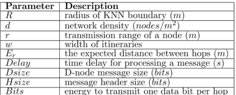
Parameter Description

R radius of KNN boundary (m)

d network density (nodes/m2) r transmission range of a node (m)

w width of itineraries

Er the expected distance between hops (m)

Delay time delay for processing a message (s) Dsize D-node message size (bits)

Hsize message header size (bits)

Bits energy to transmit one data bit per hop

Table 3.1: Parameters used in our analytical model.

circle j+1 circle j Qn+1 Qn itinerary j w Er Er

Figure 3.3: Information statistics in routing path.

able to estimate while routing KNN query and will be described later. Assumptions made in our analysis are discussed as follows. We assume that sensor nodes are uniformly distributed and there is no void area in the monitored region. Message transmissions are reliable, i.e., there is no message lost. Query propagation along the branch- and return- segments are one hop for each concentric circle and each Q-node is ideally located in the itineraries. Parameters used in our analysis are summarized in Table 3.1

3.3.2 Minimum Latency for PCIKNN

In PCIKNN, when the number of sectors is increased, peri-segment is expected to shorten, thus reducing the latency. For each sector, once a KNN query arrives boundaries among sectors, the partial results should be transmitted to the home node along the return-segments. With a larger number of sectors, network jams are likely to happen around the home node, degrading the latency of PCIKNN. Therefore, the latency time of PCIKNN mainly depends

on two values: latencyperiand latencyhome. Explicitly, latencyperiis the latency of propagating

KNN query in peri-segments at the farthest concentric-circle from the home node because the latency of query propagation along peri-segments at the inner concentric-circle is smaller. On

the other hand, latencyhome is the time spent for processing partial results at the home node.

Therefore, the latency time of PCIKNN is formulated as

(25)

To calculate latencyperi, we should take into account message delays for sending probe

messages and receiving D-nodes messages at each Q-node. Thus, we could have latencyperias

follows:

latencyperi= Ehopperi× (1 + E

peri

Dnum) × Delay

, where E_hopperiis the expected number of Q-nodes in the peri-segment at the farthest

concentric-circle and E_Dperi_num is the expected number of D-nodes of a Q-nodes. The expected number of

D-nodes is estimated as the number of D-nodes in the gray area in Figure 3.3. Consequently, we have

E_hopperi= 2 × π × R × w

2 × S × Er

E_Dperi_num _{= Er × w × d}

, where Er is the expected length of each hop of Q-nodes. According to [27][28], Er is

formulated as Er = r2√_{d/(1 + r}√_d).

As for the latency time spent on collecting partial results at the home node, we assume that partial results are sent to the home nodes at the same time (which is the worst-case scenario). Hence, we have the following latency:

latencyhome = 2 × S × Delay

According to the above derivations, the latency time for PCIKNN is able to derived as follows:

latency = (π×R

S×Er × (1 + w × Er × d) × Delay) + (2 × S × Delay)

In order to obtain the optimal number of sectors to achieve the minimal latency time of PCIKNN, we could differentiate the above latency formula. Therefore, the optimal number of sectors is derived as follows:

S =r (

π×R

Er ) × (1 + w × Er × d)

2

3.3.3 Minimum Energy for PCIKNN

As mentioned above, a long itinerary length shall incur more energy consumption. However, the energy consumption of PCIKNN should consider the energy consumption on the query propagation and data collection along with branch- and peri-segments, and the energy

(26)

con-carrying data collected from D-nodes. On the contrary, a large number of sectors increases the number of branch-segments and return-segments, incurring more energy consumption over-head on the query propagation and data collection along branch-segments, and the partial result collection along return-segments. Thus, an optimal number of sectors can be derived to minimize the energy consumption. Generally speaking, the energy consumption of PCIKNN involves two parts in each itinerary segment: 1) Data collected from D-nodes should be car-ried hop-by-hop along with KNN query. 2) KNN query is propagated along with Q-nodes. Without loss of generality, the energy consumption is modeled as the communication cost in terms of the number of bits transmitted among sensor nodes. Thus, the energy consumption of PCIKNN is the sum of energy consumption corresponding to branch-segment, peri-segment and return-segment of all sectors. Since there are multiple concentric-circle itineraries in PCIKNN, the energy consumption on the type-segment in the i th concentric-circle itineraries

is expressed by energytype,Ci. For example, the energy consumption of peri-segment itineraries

in the first concentric-circle is represented as energy_peri,C₁. Consequently, we have

energy =PR/w

i=1(S × (energybranch,Ci+ energyperi,Ci+ energyreturn,Ci)),

where the number of concentric-circles is R

w.

The energy consumption is modeled as Ehop × Bits, where Ehop is the expected number

of hops and Bits is the energy consumption to transmit one data bit per hop. Let E_hop,Citype

denote the expected number of hops in the type-segment on Ci. For example, Ebranch

hop,Ci is the

expected number of hops in the branch-segment on Ci. Furthermore, E_Dtype_num represents the

expected number of D-nodes of a Q-node in the type-segment. For computation simplification, we simplify the radius of Ci is i × w. In the following, we will derive the energy consumption in each itinerary segment.

Note that the energy consumption in each segment consists of D-nodes data carrying energy and Q-nodes query propagation energy. For the energy consumption for the branch segment on Ci, we could have the following formula:

Ebranch

hop,Ci × (Hsize+ (EDbranchnum × Dsize)) × Bits,

where Ebranch

hop,Ci = 1, EDbranchnum = 0 since Q-nodes are assumed to be connected hop-by-hop along

with a branch-segment and D-nodes data collected are divided into peri-segments. Similar, we could derive the energy consumption in the peri-segment as follows:

2 × ((Ehop,Ciperi × Hsize) + ((P

E_hop,Ciperi

j=1 (j × E

peri

Dnum)) × Dsize)) × Bits,

where E_hop,Ciperi = 2 × π × i × w

2 × S × Er and E

peri

(27)

Since we have two return-segments in each sector, the energy consumption is modeled as follows:

2 × Ereturn

hop,Ci× (Hsize+ (EDreturnnum,Ci× Dsize)) × Bits,

where Ereturn

hop,Ci = i, EDreturnnum,Ci = E

peri hop,Ci× E

peri Dnum.

Putting the above formulas together, we could further utilize differentiation to derive the optimal number of sectors so as to minimize the energy consumption of PCIKNN. Conse-quently, the optimal number of sectors is derived as follows:

S = v u u t π2_w3_d Er × (2R w + 1) 6 × Dsize Hsize

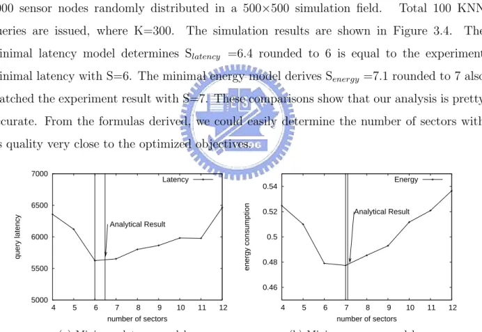
Model Validation: The simulation environment for model validation is that there are

1000 sensor nodes randomly distributed in a 500×500 simulation field. Total 100 KNN

queries are issued, where K=300. The simulation results are shown in Figure 3.4. The

minimal latency model determines Slatency =6.4 rounded to 6 is equal to the experiment

minimal latency with S=6. The minimal energy model derives Senergy =7.1 rounded to 7 also

matched the experiment result with S=7. These comparisons show that our analysis is pretty accurate. From the formulas derived, we could easily determine the number of sectors with its quality very close to the optimized objectives.

5000 5500 6000 6500 7000 4 5 6 7 8 9 10 11 12 query latency number of sectors Analytical Result Latency

(a) Minimum latency model

0.46 0.48 0.5 0.52 0.54 4 5 6 7 8 9 10 11 12 energy consumption number of sectors Analytical Result Energy

(b) Minimum energy model

(28)

Chapter 4 KNN Boundary Estimation

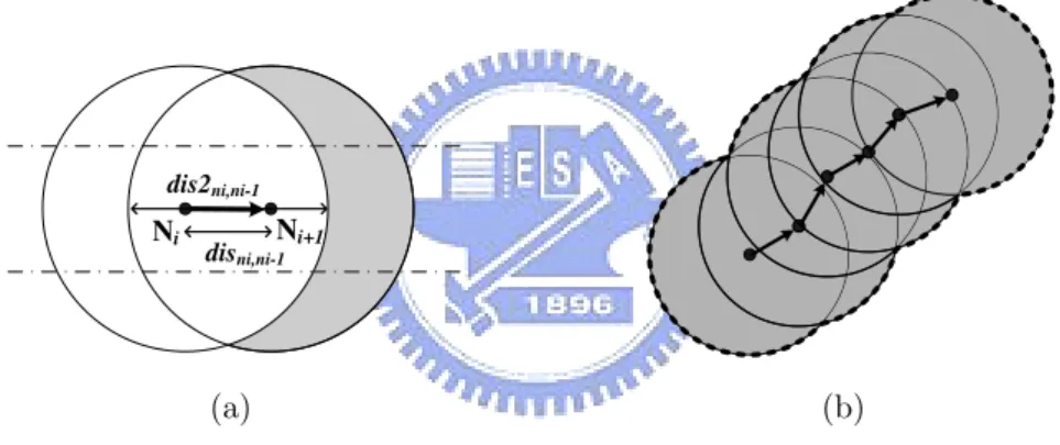
Obviously, the precision of the KNN boundary estimation has a direct impact on the perfor-mance of itinerary-based KNN query processing. In this chapter, we develop a mechanism to estimate KNN boundary. Ni+1 Ni dis2ni,ni-1 disni,ni-1 (a) (b)

Figure 4.1: Estimating coverage areas of routing.

4.1 Design of KNN Boundary Estimation

An over-estimated KNN boundary will lead to excessive energy consumption and long latency, whereas an under-estimated KNN boundary may reduce the accuracy of query results. Thus, boundary estimation is very critical to the success of itinerary-based KNN query processing. Here we assume that sensor nodes do not have a priori knowledge about the density and distribution of nodes in the network. To address this issue, DIKNN [27][28] first collects (partial) network information in the query routing phase to derive the network density, which in turn is used to estimate a boundary that are likely to contain K sensor nodes. Clearly, how to precisely determine the network density from the partial information gathered in the routing phase is important. In the following, we will describe our approach to derive the

(29)

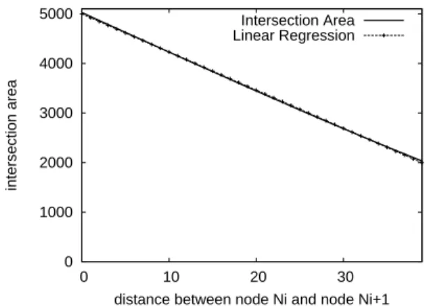
0 1000 2000 3000 4000 5000 0 10 20 30 intersection area

distance between node Ni and node Ni+1 Intersection Area Linear Regression

Figure 4.2: Intersection covered area with various node distances.

network density in the routing phase.

By using a geo-routing protocol, e.g., GPSR, a KNN query is greedily forwarded from the source node to the home node. In the routing phase, network information, such as the number of nodes and the coverage area shown the dotted area in Figure 4.1(b) along the routing path, is obtained. This information (i.e., coverage area of routing and the number

of nodes encountered) are gathered and sent along with KNN query. Let Ai denote the area

covered by relay messages up to the ith hop and N um represents the total number of nodes within the coverage area of the routing path. They are collected and updated as a KNN query moves forward hop-by-hop. Once the query reaches its home node, the collected information is used to estimate the network density.

Next, we demonstrate how to update these two values in the routing phase. A message

relay from node Ni to node Ni+1 is shown in Figure 4.1(a), where the gray area is the newly

explored area, denoted as EAi. The number of sensor nodes in EAi is denoted by inci+1.

By adding inci+1 to Num, one could have the most updated number of nodes encountered so

far. The value of EAi is formulated as EAi = πr2− H(2r − dist(Ni, Ni+1)), where r is the

transmission radius of a sensor, H(.) is a linear function and dist(Ni, Ni+1) is the Euclidean

distance between Ni and Ni+1. By extensive experiments, we observed that the intersection

area between two sensor nodes is almost negative correlated with dist(Ni, Ni+1) shown in

Figure 4.2. Thus, in this paper, to precisely estimate the intersection area between two sensor nodes, we explore linear regression techniques and H(.) is thus formulated as:

H(dist(Ni, Ni+1)) = c1+ c2× dist(Ni, Ni+1),

(30)

hop is as follows:

Ai = EAi+ Ai−1, for i > 1 and A1 = πr2.

When a KNN query reaches the home node, the home node computes the network density

D as D=N um_A , where A is the total area covered by relay messages from the source node. As

a result, the KNN boundary is estimated as follows:

πR2_{× D = K}

R =qK

πD.

Although DIKNN[27][28] also explores the network density to estimate the KNN boundary region, an additional list is used to record all local information of each hop in the routing phase. This list, sent along with KNN query, incurs more energy overhead. Furthermore, DIKNN estimates KNN boundary by an algorithm named KNNB presented in their paper which estimates the KNN boundary by local information hop by hop started from the home node to extend the estimated boundary until a circle centered by query point q is found and has K nodes. Obviously, there two condition of boundary estimation by KNNB, first, KNNB may utilize less local information to estimated the KNN boundary when the estimated KNN boundary is smaller than the length of routing path. It may reduce the accuracy because KNN uses less local information for boundary estimation. Second, there is a problem when the additional list is too short to find the KNN boundary. We compare the performance of our proposed mechanism with that of DIKNN later.

(31)

Chapter 5 Mechanisms for Spatial Irregularity

The above boundary estimation is under the assumption that the sensor nodes are uniformly distributed in the monitored region. However, it is possible that real sensor networks are spatial irregular, thereby reducing the accuracy of boundary estimation. To deal with this problem, in this chapter, we present a mechanism to dynamically adjust the estimated KNN boundary when the query is propagated. Furthermore, in PCIKNN, the home node will collect KNN query results via the return-segment in each sector. Therefore, the home node will decide whether KNN query should be propagated or not according to the partial KNN query results collected. We, therefore, propose two mechanisms for the two modes (i.e., the min energy model and the min latency mode).

5.1 Adjusting Estimated KNN Boundary During Query

Propagation

After estimating the KNN boundary with radius R , KNN query is then propagated to branch-segments. The network information obtained in the routing phase (i.e., the total coverage area A and the number of nodes Num) is sent with KNN query processing. When KNN query is propagated along with the branch-segment, local network information within the segment is

accumulated via the below operation in the routing phase. AB (respectively, N umB) is the

coverage area (respectively, number of nodes) along the branch-segment. Consequently, we could derive the network density by exploring local network information. Hence, the network density is updated as follows:

(32)

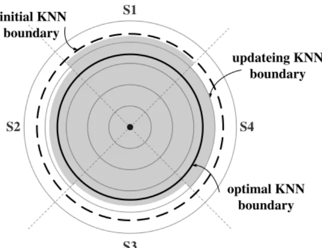
S1 S2 S4 S3 initial KNN boundary optimal KNN boundary updateing KNN boundary

Figure 5.1: Updating KNN boundary dynamically.

By exploiting local network information in each sector, PCIKNN is able to dynamically adapt KNN boundary. For example, the gray area in Figure 5.1 is adapted to node densities in sectors. Even though this adapted KNN boundary still cannot guarantee the accuracy of KNN query result because the adapted KNN boundary still may be smaller or larger than the real KNN boundary, it is expected to decrease the difference between the estimated KNN boundary and the real KNN boundary. In the performance evaluation section, we will show the performance of estimated boundary updating.

5.2 Adjusting Estimated KNN Boundary from the Home

Node

As pointed out early, in PCIKNN, the home node has the partial KNN query results from each sector. Therefore, the home node is able to decide whether KNN query should be propagated or not according to the partial KNN query results collected. Thus, we propose two mechanisms to ensure KNN collection and handle the un-accuracy of the estimated KNN boundary. Due to the nature of PCIKNN, partial results from each sector are collected by the home node, the home node is able to decide and control whether the estimated boundary should be extended or the query processing should be stopped via controlling messages sent by the home node. Mechanism for the Min Energy Mode:

In the min energy mode of PCIKNN, the goal is to conserve as much energy as possible. Therefore, only receiving control messages (referring to CONTINUE message) from the home node, Q-nodes alone with the branch-segments are propagated to the next concentric circles. Specifically, when the home node receives partial results from each sector, the home node will

(33)

record some information, such as the sector and the concentric-circle, that indicate where the partial result comes from. Once the home node collect all the partial results from each sector in a concentric-circle Ci, the home node will determine whether the KNN query should be propagated in the next concentric-circle Ci + 1 or not. Note that, when KNN query reaches or exceeds the estimated KNN boundary, the Q-nodes will wait for the control messages from the home node. It can be seen that the KNN query is disseminated concentric-circle by concentric-circle after the KNN query exceeds the estimated KNN boundary. On the other hand, when the partial results from sectors fulfil the KNN requirement, the home node informs the Q-nodes to stop the KNN query dissemination and data collection in each sector, saving the energy consumption.

Mechanism for the Min Latency Mode:

The goal of this mechanism is to minimize the query latency under decreasing unnecessary search overhead and thus, the home node frequently broadcasts the radius of the estimated KNN boundary once receiving the partial KNN results. Explicitly, the home node broad-casts information related to the current status of KNN query results and allow Q-nodes to quickly propagate KNN query. Hence, when a partial result is collected, the home node will estimate the distance between the Kth data and the query point (referred to DMAX) and DMAX is the minimal boundary estimated so far that ensures there are KNN data in this boundary. If the number of KNN results collected by the home node does not exceed K, the DMAX is set to infinite. Note that the DMAX will be updated if the partial KNN results are collected. Then, if the current value of DMAX is different from previous-round DMAX, the home node broadcasts messages that contain the current DMAX to Q-nodes. Otherwise, the home node sends a message to Q-nodes about the location information of the partial results collected. A KNN query stops disseminating when the home node ensures that KNN results are collected. In particular, when a Q-node on a branch-segment exceeds the estimated KNN boundary, this Q-node holds an estimated short period WAIT TIME for waiting the home node message. The estimated period WAIT TIME is sum of the estimated query dissemina-tion time of peri-segment, the partial result returning along return-segment and the estimated message broadcasting time along the branch-segment. Furthermore, when a Q-node receives the DMAX message, if the distance between the home node and this Q-node is larger than DMAX, the KNN query stops the query propagation to avoid unnecessary searching.

(34)

is referred as Over Cnum, and Over Ci means the i th concentric-circle that exceeds the estimated KNN boundary, and there are S sector. In min energy mechanism, the home node broadcasts for each exceeded circle and each sector. Hence, the broadcasting messages number is S × Over Cnum. In min latency mechanism, there is an obvious upper bound of the broadcasting time, when each partial result updates DMAX. In this condition, there are S × Over Cnum partial results, and each time of broadcasting is sent for each sector. As a result, the number of broadcasting messages is S × Over Cnum × S. Obviously, the mechanism in the min energy mode may broadcast less messages and consumes less energy for controlling query processing.

For the latency analysis, the total additional waiting time of mechanisms is used as the

analytical latency time. LatencyBj,Over Ci denotes the processing latency of the j th

branch-segment in the i th exceeding circle and the value of LatencyBj,Over Ci consists of three factors:

the latency of peri-segments, the latency of return-segments and the latency of broadcasting along with branch-segments. Thus, we have

LatencyBj,Over Ci = Latencyperi,Over Ci+ Latencyreturn,Over Ci+ M sg BroadcastingOver Ci

In the min energy mechanism, because the KNN query is propagated circle by circle, the additional latency is formulated as the summation of holding times of each circle:

Latencymin energy =POver Cnumi=1 (HoldingOver Ci)

, where HoldingOver Ci denotes the holding time of the i th concentric-circle. Clearly, the

holding time of each sector in a concentric-circle is determined by the maximal LatencyBj,Over Ci

among each sector and is derived as,

HoldingOver Ci = max1≤j≤S(LatencyBj,Over Ci)

In the min latency mechanism, because the waiting time of each branch-segment is un-affected with each other, the additional latency is the maximal waiting time of among all segments, which is the summation of waiting time of each circle along the branch-segment. Thus, we have,

Latencymin latency = max1≤j≤S(POver Cnumi=1 (W aitingBj,Over Ci))

, where W aitingBj,Over Ciis the waiting time of the j th branch-segment in the i th

concentric-circle and is set to the minimum value between the estimated waiting time and real processing latency.

(35)

W aitingBj,Over Ci = M IN {W AIT T IMEBj,Over Ci, LatencyBj,Over Ci}

Note that for the mechanism in the min latency mode, once one partial result is col-lected, the home node informs other Q-nodes the status of KNN results and Q-nodes will determine whether KNN query threads should be propagated or not. For the mechanism in the min energy mode, the goal is to conserve as much energy as possible. Therefore, KNN query threads is propagated after all the partial results in the previous concentric-circles are

collected. Obviously, the waiting time W aitingBj,Over Ci in the min latency mechanism is

smaller than the holding time HoldingOver Ci in the min energy mechanism. According to the

formulas derived above, it can be seen that the latency in the min latency mode is smaller than that in the min energy mode.

(36)

Chapter 6 Performance Evaluation

We develop a simulation to evaluate the performance of PCIKNN and other closely related works, i.e., IKNN and DIKNN. The simulation model and parameter settings are presented in Section 6.1. The experimental results are reported in Section 6.2.

6.1 Simulation Model

Our simulation is implemented in CSIM[21]. There are 1000 sensor nodes randomly distributed

in a 500×500m2 _{region. The transmission radius of a node is 40m. For each sensor node, the}

average number of neighboring nodes is 20. The message delay for transmitting or receiving messages is 30ms. Sensor nodes to be static in the default environment. For each query, the location of a query point q is randomly selected. The value of K for each KNN query is 100. The beacon message broadcasting period is 3s. A KNN query is answered when the query result is returned to the source node. For each round of experiment, 5 queries are issued from randomly selected source nodes. Each experimental result is obtained by average of fifty rounds of experiments. Three itinerary-based KNN algorithms are implemented. Algorithm IKNN [30] exploring one itinerary is adopted while Algorithm DIKNN [27][28] with minimum latency is utilized. For fair comparison, we derive the result of DIKNN with all possible number of sectors and find out that the results with minimum latency are almost the same with minimum energy. So that, we just show the result with minimum latency in DIKNN. In Algorithm PCIKNN, we derive results in minimum latency mode adopted the min energy mechanism and in minimum energy mode adopted the min latency mechanism. We compare three algorithms in terms of energy consumption, query latency and query accuracy under various environment factors such as the network density, the number of sample size (i,e., K for KNN queries), the node mobility and the failure rate of nodes. These performance metrics

(37)

are summarized as follows:

Energy Consumption (Joules): The total amount of energy consumed for processing a KNN query in a simulation run.

Query Latency (ms): The elapsed time between the time a query is issued and the time the query result is returned to the source node.

Query Accuracy(%): The percentage ratio of the number of sensor nodes that are exactly the K nearest sensor nodes to query point q over the number of sensor nodes in KNN query results collected.

6.2 Experimental Results

In this section, we first investigate the impact of network density on the three examined algorithms. Next, we study the scalability of these three algorithms to the value of K. Then we show the performances under varied node mobility and node failure rate. Finally, we examine the accuracy of boundary estimation.

6.2.1 The Impact of Network Density

First, we investigate the impact of network density to the performance of the three examined algorithms. Here, the network density is measured as the number of sensor nodes deployed

in a fixed monitored region (i.e., 500×500m2_{). We vary the number of sensor nodes from}

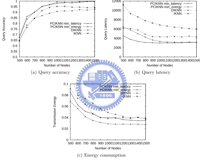
500 to 1500. As a result, the average number of neighbors for each node is varied from 10 to 30. Figure 6.1(a) shows that all three algorithms have better query accuracy when the network density is increased. However, when the network is sparse (i.e., the number of nodes is smaller than 800 nodes), PCIKNN outperforms IKNN and DIKNN. This is because a KNN query propagating along itineraries in IKNN and DIKNN may easily get dropped because they have longer itineraries than PCIKNN. Due to the high parallelism in itineraries, the length of each segment of itineraries is shorter, and this reason causes that PCIKNN is robust. Only a few D-nodes are lost if a KNN query thread is dropped. Furthermore, DIKNN utilizes the estimated KNN boundary to decide whether KNN query should be stopped or not (i.e., without guaranteed mechanisms like PCIKNN). Consequently, the query accuracy of DIKNN is significantly reduced because of spatial irregularity. In a fairly dense network (i.e., the number of nodes is larger than 900 nodes), both IKNN and PCIKNN have better

(38)

0.5 0.55 0.6 0.65 0.7 0.75 0.8 0.85 0.9 0.95 1 500 600 700 800 900 1000 1100 1200 1300 1400 1500 Query Accuracy Number of Nodes PCIKNN min_latency PCIKNN min_energy DIKNN IKNN

(a) Query accuracy

0 2000 4000 6000 8000 10000 12000 500 600 700 800 900 1000 1100 1200 1300 1400 1500 Query Latency Number of Nodes PCIKNN min_latency PCIKNN min_energy DIKNN IKNN (b) Query latency 0 0.02 0.04 0.06 0.08 0.1 500 600 700 800 900 1000 1100 1200 1300 1400 1500 Transmission Energy Number of Nodes PCIKNN min_latency PCIKNN min_energy DIKNN IKNN (c) Energy consumption

(39)

of concurrent KNN query propagation. The latency is lower when the number of nodes is increased for each algorithm. In the dense network, the latency of three algorithms tends to decrease. Clearly, in a dense network, KNN boundary is small, leading to a short latency. Figure 6.1(c) shows the energy consumption of three algorithms. PCIKNN has the lowest energy consumption, showing the merits of itinerary designed in PCIKNN.

6.2.2 Scalability of IKNN, DIKNN and PCIKNN

0.5 0.55 0.6 0.65 0.7 0.75 0.8 0.85 0.9 0.95 1 50 100 150 200 250 300 350 400 Query Accuracy K PCIKNN min_latency PCIKNN min_energy DIKNN IKNN

(a) Query accuracy

0 5000 10000 15000 20000 25000 30000 50 100 150 200 250 300 350 400 Query Latency(ms) K PCIKNN min_latency PCIKNN min_energy DIKNN IKNN (b) Query latency 0 0.1 0.2 0.3 0.4 0.5 0.6 0.7 50 100 150 200 250 300 350 400

Transmission Energy Consumption(J)

K PCIKNN min_latency PCIKNN min_energy DIKNN IKNN (c) Energy consumption Figure 6.2: Impact of K.

Next, we investigate the impact of sample size K to scalability of the three algorithms. Clearly, K has a direct impact on the number of nodes involved in query processing. In this experiment, the value of K is varied from 50 to 400. The query accuracy of IKNN, DIKNN and PCIKNN is shown in Figure 6.2(a). It can be seen in Figure 6.2(a) that the query accuracy of DIKNN is significantly reduced as K increases, because the KNN query result of each itinerary in DIKNN is directly sent back to the source without further processing even though

(40)

query accuracy under the varied K because they both have KNN guaranteed mechanisms. The latency increases as K increases since more sensor nodes are discovered. As can be seen in Figure 6.2(b), PCIKNN has the smallest latency, validating our analytical model for minimum latency of PCIKNN. As seen in Figure 6.2(c), energy consumption of all algorithms tends to increase as K increases because the number of sensor nodes involved is increased as well. PCIKNN has the smallest energy consumption. Furthermore, compared with PCIKNN with the minimum latency mode (i.e., PCIKNN min latency), PCIKNN with the minimum energy (i.e., PCIKNN min energy) indeed has the minimal energy consumption, showing the correctness of our optimized derivation.

6.2.3 Impact of Node Mobility

0 0.2 0.4 0.6 0.8 1 1 3 5 7 9 11 13 15 Query Accuracy Nodes Mobility (m/s) PCIKNN min_latency PCIKNN min_energy DIKNN IKNN

(a) Query accuracy

2000 4000 6000 8000 10000 12000 1 3 5 7 9 11 13 15 Query Latency(ms) Nodes Mobility(m/s) PCIKNN min_latency PCIKNN min_energy DIKNN IKNN (b) Query latency 0.02 0.04 0.06 0.08 0.1 0.12 1 3 5 7 9 11 13 15 Transmission Energy(J) Nodes Mobility(m/s) PCIKNN min_latency PCIKNN min_energy DIKNN IKNN (c) Energy consumption

Figure 6.3: Impact of node mobility.

The third experiment we investigated is the impact of node mobility for three algorithms. Obviously, when the mobility gets higher, the accuracy gets lower, because two reasons: first, the rate of queries and messages lost increase because each node doesn’t have its current neighbors information. Second, a node which is in the K nearest neighbors to the query point

(41)

q may move out. In this experiment, the mobility of node is varied from 1m/s(i.e., walking speed) to 15m/s(i.e., driving speed). The accuracy result is shown in Figure 6.3(a) and it can be seen that the accuracy of three algorithms decrease seriously when the mobility increases. However, it shows that PCIKNN still has the best query accuracy in both in min latency and min energy modes. The reason is that PCIKNN has highly parallelism to decrease the latency and be more robust because the length of an itinerary is much less then IKNN’s and DIKNN’s. By the way, the query lost rate in routing phase is about 25% when the speed is 15m/s, and this accuracy lost is caused by geo-routing algorithms. The latency results shown in Figure 6.3(b) get higher when the mobility is higher in each algorithm. Because even a query thread is dropped the source node in IKNN and DIKNN or the home node in PCIKNN should wait a threshold time to ensure the query processing is failed. It makes the latency worsen, but PCIKNN still outperforms others. The energy consumption results also increase with the mobility shown in Figure 6.3(c). The mobility increasing causes a Q-node may move out its original itinerary region easily and the Q-node should take effort to disseminate the query back to its original itinerary. However, PCIKNN still has the best energy consumption in min energy mode.

6.2.4 Impact of Node Failure

Next, we investigate the impact of node failure to the performance of the three examined algorithms. In this experiment, the failure rate of node is varied from 0.1% to 0.5% and the time period for each node to check whether it fails is 300ms. Obviously, a node failure has directly impact of query processing. The home node, the source node or the routing node on the routing path failure causes the query dropped; a Q-node failure causes its query thread dropped and decreases the query accuracy; a D-node failure causes KNN result changed. The result of query accuracy is shown in Figure 6.4(a). It can be seen that PCIKNN has the best accuracy performance which is still upper than 80% when the failure rate is high (i.e., 0.5%). PCIKNN is the most robust because of its highly parallelism to decrease the latency and the length of an itinerary is much less then IKNN’s and DIKNN’s. The latency and energy consumption results of each algorithm both get higher when the failure rate increase shown in Figure 6.4(b) and Figure 6.4(c). The reason is the same with the result of the node mobility experiment. It can be soon that PCIKNN still has the best performance and is impacted by the node failure rate slightly.

(42)

0.5 0.55 0.6 0.65 0.7 0.75 0.8 0.85 0.9 0.95 1 0 0.1 0.2 0.3 0.4 0.5 Query Accuracy Fail Rate(%) PCIKNN min_latency PCIKNN min_energy DIKNN IKNN

(a) Query accuracy

2000 4000 6000 8000 10000 12000 0 0.1 0.2 0.3 0.4 0.5 Query Latency(ms) Fail Rate(%) PCIKNN min_latency PCIKNN min_energy DIKNN IKNN (b) Query latency 0 0.02 0.04 0.06 0.08 0.1 0.12 0 0.1 0.2 0.3 0.4 0.5

Transmission Energy Consumption(J)

Fail Rate(%) PCIKNN min_latency PCIKNN min_energy DIKNN IKNN (c) Energy consumption

(43)

100 120 140 160 180 200 220 240 500 600 700 800 900 1000 1100 1200 1300 1400 1500

search region’s radius

number of nodes OPTIMAL

PCIKNN DIKNN

Figure 6.5: KNN boundary estimation of DIKNN and PCIKNN.

6.2.5 KNN Boundary Estimation Simulation

To evaluate the proposed KNN boundary estimation technique, we set the value of K to be 300. To avoid the effect of network boundary, query points in the middle region (i.e., 100m×100m)

are selected. The liner regression function of PCIKNN is set to H(dist(Ni, Ni+1)) = (−76.9166×

dist(Ni, Ni+1) + 4999.0903) by liner regression technique in [12]. The optimal KNN boundary

is the average distance of k th distant nodes of all queries derived by the experiments. As shown in Figure 6.5, PCIKNN is very close to the optimal KNN boundary under various network density. However, the boundary estimated in DIKNN does not fit well with the trend of the optimal KNN boundary. Moreover, in Figure 6.5, when the number of nodes is smaller than 800, the KNN boundary estimated in DIKNN is smaller than the optimal value because the KNN boundary is large and the routing path from the source node to the home node is not long enough to estimate a region contained K sensor nodes. On the other hand, even though the routing path is long enough to estimate the KNN boundary, the result is not precise due to the inaccuracy of coverage areas in routing path. Figure 6.5 demonstrates the correctness and the accuracy of our KNN boundary estimation.

6.2.6 KNN Boundary Adjusting Simulation

In the final experiment, we evaluate the performance of the mechanisms adjusting the KNN boundary by the home node. We set the value of K to be 300, and the result shown in Figure 6.6. It shows that the accuracy without adjusting the KNN boundary by the home node gets worse when the value of K increases. It is because that when the K increases, the difference between the real KNN boundary and the estimated boundary impacts the accuracy

(44)

0.7 0.75 0.8 0.85 0.9 0.95 1 50 100 150 200 250 300 350 400 Query Accuracy K min_latency min_energy min_latency without mechanism min_energy without mechanism

Figure 6.6: KNN boundary adjusting mechanisms by the home node in PCIKNN.

and Min energy, just about 0.1% and 1%. It can be seen that the adjusting mechanisms of the home node maintains the accuracy and these mechanisms cause slight overhead.

(45)

Chapter 7 Conclusions

In this paper, we proposed an efficient itinerary-based KNN algorithm, PCIKNN, for KNN query processing in the sensor network. PCIKNN disseminates queries and collects data along pre-designed itineraries with high parallelism. We derived the latency and the energy con-sumption of PCIKNN and then by optimizing the derived formulas, we are able to determine the appropriate number of sectors for PCIKNN. Furthermore, by exploring linear regression, the KNN boundary estimated is as close as the optimal one. In addition, PCIKNN is able to dynamically adjust KNN boundary by considering local network information within sec-tors. Furthermore, KNN query is guaranteed to be answered since the home node will decide whether to further extend the boundary or not based on collected KNN query result. Exten-sive experiments have been conducted. Experimental results show that PCIKNN significantly outperforms others in terms of energy consumption, query latency and query accuracy.

(46)

Bibliography

[1] R. Benetis, C. S. Jensen, G. Karciauskas, and S. Saltenis. Nearest Neighbor and Reverse Nearest Neighbor Queries for Moving Objects. In Proc. of 6th International Symposium on Database Engineering & Applications Symposium (IDEAS), pages 44–53, 2002. [2] M. Demirbas and H. Ferhatosmanoglu. Peer-to-Peer Spatial Queries in Sensor Networks.

In Proc. of the 3rd International Conference on Peer-to-Peer Computing (P2P), page 32, Washington, DC, USA, 2003. IEEE Computer Society.

[3] D. Estrin, R. Govindan, and J. Heidemann. Next Century Challenges: Scalable Coordi-nation in Sensor Networks. In Proc. of the 5th ACM/IEEE InterCoordi-national Conference on Mobile Computing and Networking (MobiCom), pages 263–270, 1999.

[4] H. Ferhatosmanoglu, E. Tuncel, D. Agrawal, and A. E. Abbadi. Approximate Nearest Neighbor Searching in Multimedia Databases. In Proc. of the 17th IEEE International Conference on Data Engineering (ICDE), pages 503–511, 2001.

[5] D. Goldin, M. Song, A. Kutlu, H. Gao, and H. Dave. Georouting and Delta-gathering: Efficient Data Propagation Techniques for Geosensor Networks. In NSF Worshop on GeoSensor Networks, 2003.

[6] A. Guttman. R-Trees: A Dynamic Index Structure for Spatial Searching. In Proc. of the ACM Special Interest Group on Management Of Data International Conference (SIGMOD), pages 47–57, 1984.

[7] W. R. Heinzelman, A. Chandrakasan, and H.balakrishnan. Energy-Efficient Communi-cation Protocol for Wireless Microsensor Networks. In Proc. of the 33rd Hawaii Interna-tional Conference on System Sciences (HICSS), pages 8020–8029, 2000.

[8] G´ısli R. Hjaltason and Hanan Samet. Distance browsing in spatial databases. ACM Transactions on Database Systems, 24(2):265–318, 1999.

平行化路徑式KNN查詢演算法運用於無線感測器網路

國

立

交

通

大

學

資訊科學與工程研究所

碩

士

論

文

平行化路徑式ＫＮＮ查詢演算法運用於無

線

感

測

器

網

路

Parallel Itinerary-based KNN Query Processing in

Wireless Sensor Networks

研 究 生：傅道揚

指導教授：彭文志 教授

96

碩

士

論

文

96

碩

士

論

文

96

碩

士

論

文

96

碩

士

論

文

96

碩

士

論

文

傅道揚

9555514

傅道揚

9555514

傅道揚

9555514

傅道揚

9555514

傅道揚

9555514

平行化路行式 KNN 查詢演算法運用於無線感測器網路

Parallel Itinerary-based KNN Query Processing in

Wireless Sensor Networks

研 究 生：傅道揚 Student：Tao-Yang Fu

指導教授：彭文志 Advisor：Wen-Chih Peng

國 立 交 通 大 學

資 訊 科 學 與 工 程 研 究 所

碩 士 論 文

Contents

List of Figures

List of Tables

Chapter 1

Introduction

Chapter 2

Preliminaries

2.1

Assumptions

2.2

Query Dissemination Phase in Itinerary-based KNN

Query Processing

2.3

Overview of PCIKNN

研究生：傅道揚

指導教授：彭文志教授

研究生：傅道揚 Student：Tao-Yang Fu

國立交通大學

資訊科學與工程研究所

碩士論文