力回饋方向盤於虛擬實境之發展

全文

(1)國立交通大學機械工程研究所碩士論文力回饋方向盤於虛擬實境之發展 A Force Feedback Wheel Developing for Virtual Environment. 研究生 : 吳秉霖指導教授 : 成維華. 博士. 中華民國九十三年六月.

(2) 力回饋方向盤於虛擬實境之發展 A Force Feedback Wheel Developing for Virtual Environment. 研究生：吳秉霖. Student：Bing-Ling Wu. 指導教授：成維華博士. Advisor：Dr. Wei-Hua Chieng. 國立交通大學機械工程學系碩士論文. A Thesis Submitted to Department of Mechanical Engineering College of Electrical Engineering National Chiao Tung University in partial Fulfillment of the Requirements for the Degree of Master in Mechanical Engineering June 2004 Hsinchu, Taiwan, Republic of China. 中華民國九十三年六月.

(3) 力回饋方向盤於虛擬實境之發展. 研究生：吳秉霖. 指導教授：成維華博士. 國立交通大學機械工程學系摘要時至今日，一般我們常見的力回饋方向盤多用於電腦賽車遊戲等娛樂設施，讓人不僅擁有視覺和聽覺的享受，還加入了觸覺感受，使用者可以玩的盡興，但由於我們所需之力回饋方向盤主要應用於虛擬實境，以提供操控功能與觸覺回饋，輔助虛擬實境視覺上的不足。一般力回饋搖桿的精密度、力矩等並不適用於精密度需求較高的虛擬實境中使用，有鑑於此我們設計了更適合於虛擬實境中使用之力回饋方向盤。本論文研究方向就是結合機電整合、PC-Based Motion Control、和虛擬實境的高度整合。對於力回饋方向盤整體系統，包含硬體構成和軟體架構，配合汽車在虛擬實境中不同的情況，藉由汽車動態模擬計算，及車輛操控系統之幾何結構，和方向盤產生相對應之力矩等做一完整的分析，並且設計其相對應之軟硬體，完成能夠即時運作整個系統。. i.

(4) A Force Feedback Steering Wheel Developing for Virtual Environment Student：Bing-Ling Wu. Advisor：Dr. Wei-Hua Chieng. Institute of Mechanical Engineering National Chiao Tung University. Abstract Up to now, we usually use force feedback steering wheels in entertainment equipments, such as computer motor racing machines, with which players can have fun, because they can see visions, hear sounds, and touch machines as well. To make up the visual defect in virtual reality, force feedback steering wheels are largely applied to it for control and tactile feedback functions as saving graces. However, the delicacy and the moment of the average force feedback steering wheels are not applicable to virtual reality, which needs extreme intricacy. Therefore, we study out a new one that will work out for it. This article will talk about the high integration of Mechatronic, PC-Based Motion Control and virtual reality. We cooperated the whole set of force feedback steering wheel, including hardware and software, with cars’ different aspects in virtual reality. By dynamic motor simulation and the geometric structure of motor controlling systems, we gave a painstaking analysis for the reaction of the force feedback steering wheel, like the relative moment. In the end, we accomplished the relative hardware and software so that we could completely run the whole system.. ii.

(5) Acknowledgement. I would like to express my gratitude toward my adviser Prof., Wei-Hua Chieng. Thanks for his instruction and concern both in class and in my life during the two years in the research institute. Because of his competent knowledge and ample experiences, my thesis could be completed successfully. I appreciate the instruction and support from my upper classmate, Chung-Shu Liao. He discussed theories and experiments with me during these two years. With his help, I smoothly solved all kinds of difficulties. Besides, I learned from him that I should take the attitude to work conscientiously and carefully on my study and work. I would like to be grateful to every upper classmate in Intelligent Mechtronical Lab, especially Yang-Hung Chang and Yong-Chieng Tong. They look after and were concerned about me on my life. I would like to thank all the classmates in my laboratory. The time with them was always full of happiness. Thanks my classmates in University for supporting and consoling me. Thanks my classmates in senior high school for encouraging me. Special thanks to Chia-Ling Lin. She helps me to check through and revise my thesis. At last, I would like to express my special gratitude toward my family, especially my parents. They exerted their efforts and love to cultivate me, so I can be who I am today. Now, I shall share with them the glory and the happiness.. iii.

(6) Contents. 摘要………………………………………………………………………….......i Abstract……………………………………………………………………...…..ii Acknowledgement………………………………………………………………iii Contents……………………………………………………………………..….iv Figures…..………………………………………………………………...……vii Tables...………………………………………………………………………..viii Chapter 1 Introduction…………………………………………………...……1 1.1 Virtual Reality……………….……………………...…………………...1 1.2 Design The Force Feedback Steering Wheel…..…….…………...……..2 1.3 Structure of The Force Feedback Steering Wheel…….…………...……3 Chapter 2 Dynamic Model of Vehicles………………………………...………5 2.1 Vehicle Physics……………………………………………………....….5 2.1.1 Introduction of The Vehicle Physics……………………….....…..5 2.1.2 Formulation of car physics………………………………….……5 2.2 Operation Models of Vehicles….…………………………………....….7 2.3 Wheel models of vehicles…………………………………………...…..8 2.3.1 Calculate the slip angle β i for each wheel……………………....8 2.3.2 Calculate the angle of inclination γ i for each wheel………....…9 2.3.3 Torque on the drive wheels……………………………………....9 2.3.4 Calculate the normal force for each wheel…………...……..…..10 2.3.5 Calculate the coefficient of friction of vehicle wheels’………....13. iv.

(7) 2.3.6 Calculate the maximum allowable longitudinal force generated by wheels……………………………………………..14 2.3.7 Calculate the longitudinal coefficient of friction µ xi and slip ratio S i for each wheel…………………………………....15 2.3.8 Calculate the longitudinal force Fci for each wheel................…16 2.3.9 Calculate the lateral force Fsi for each wheel………………….16 2.3.10 Coordinate system transformations……………………...….....17 2.4 Aerodynamic model of a vehicle…………………………...……….…18 2.5 Dynamic equations of operation model…………………………....….19 Chapter 3 Force Feedback System………………………………...………...21 3.1 The Steering System…………………………………………………...21 3.1.1 Introduction of the Steering System………………………….…21 3.1.2 The steering linkages……………………………………...…….21 3.2 Geometry……………………………………………………...……….23 3.2.1 Front Wheel Geometry…………………………………….....…23 3.2.2 Formulation of Geometry…………………………………...…..24 3.3 Steering System Forces and Moments…………………………...…...25 3.3.1 Tractive Force…………………………………………………...26 3.3.2 Lateral Force……...……………………………..............………26 3.3.3 Vertical Force………………………………………………...….27 3.3.4 Aligning Torque……………………………………………...….28 3.3.5 Rolling Resistance and Overturning Moments…….............…...28 3.4 Force Feedback On The Steering Wheel………………………..….…28 Chapter 4 Hardware Integration..………………………………...………...30 v.

(8) 4.1 Hardware Structure………………………………………………….....30 4.2 Principal Mechanism…………….………………………………….....30 4.3 Driving Device…………..………………………………………….....30 4.3.1 DC Motor………………………………………………………..31 4.3.2 PWM Motor Driver….………………………………………….31 4.4 Angular Potential Meter………………………………………………..32 4.5 Signal Process Interface………………………………………………..33 4.6 Armature control of dc motors………………………………………...34 Chapter 5 Conclusion…………………………………………………………37 References…………………………………………………………………......38. vi.

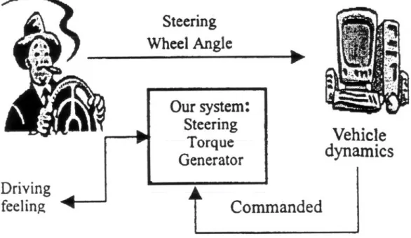
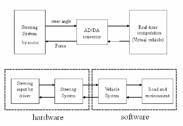
(9) Figures. Figure 1.1 Schematic diagram of the force feedback system………...………40 Figure 1.2 Schematic block diagram of the force feedback system……….....41 Figure 2.1. Operation models of vehicles………………………………...…..42. Figure 2.2 Sideslip angle……………………………………………...……...43 Figure 3.1 Illustration of typical steering systems……………………...……44 Figure 3.2 Steer rotation geometry at the road wheel…………………...…...45 Figure 3.3. Tire force and moment axis system…………………………...….46. Figure 3.4 Forces and moments acting on a right-hand road wheel………....46 Figure 3.5 Steering moment produced by tractive force………………...…...47 Figure 3.6 Steering moment produced by lateral force…………………...….48 Figure 3.7. Moment produced by vertical force acting on lateral inclination angle……………………………………………………………....49. Figure. 3.8. Moment. produced. by. vertical. force. acting. on. caster. angle………………………………………...…………………….49 Figure 3.9 Steering linkages model……………………………………….....50 Figure 4.1. Hardware Integration of steering wheel system……….…………51. Figure 4.2. Mechanism of the steering wheel…………………………...…....52. Figure 4.3 dc motor…………………………………………………………..53 Figure 4.4. A3953S…………………………………………………………...53. Figure 4.5. Angular Potential Meter………………………………………….54. Figure 4.6 ST72F651………………………………………………………...55 Figure 4.7. Armature-Control dc motors……………………………………...56. Figure 4.8 block diagram…………………………………………………….56 vii.

(10) Tables. Table 4.1 Specification of dc motor……………………………………………56. viii.

(11) Chapter 1 Introduction. 1.1 Virtual Reality We live in an era of increased computer usage in all fields of life range from personal finance, to healthcare, to manufacturing, and entertainment. Today computers are not only faster and less expensive, but communicate with us in more sophisticated way. Compact disk-based multimedia has allowed human-computer interaction through text, compressed graphical animation, stereo sound and live video images. A technological revolution is now taking place in which the user’s interaction with computer is mediated by an artificial or “virtual reality” [1, 2, 3]. Virtual Reality is super to other forms of human-computer interaction since it provides a real-time environment integrating several new communication modalities. These include stereo graphics [4], three-dimensional sound [5, 6], and tactile feedback [7, 8]. Yet, there still exist at least two aspects that prevent Virtual Reality (VR) from reaching its full potential. The first involves complexity of the scene graphics, which creates the level of visual realism of the virtual world. At present, scene complexity is limited by computer performance. It is still not possible to have both real-time and complex worlds in the same simulation, forcing designers to sacrifice visual realism for high frame-update rate. Real-time graphics require at least 15 frames/sec [9], and preferably 30 frames/sec, limiting scene complexity to between five and ten thousand polygons, depending on the computer used. The doubling in processor power that occur each few years is expected to solve the need for visual realism, 1.

(12) although it will take time to reach the required 40 million triangles/sec/eye estimated by some researchers [10]. In today’s commercial VR simulations, users can usually pass through walls, lift but not feel the weight and compliance of grasped objects, and so on. Physical characteristics can be neglected in simple “fly-by” simulations or video games; however, they become critical in applications where the user actively manipulates the simulated world, a typical example being surgical simulators. It is difficult and unreasonable to train a doctor to properly execute a given procedure, without giving him the feel of the organ being cut, of an artery pulse, or of a malignancy’s harder consistency within its softer surrounding tissue. To provide sufficient realism, the simulation must include physical constraints [11] such as object rigidity, mass and weight, friction, dynamics, surface characteristics, and so on. Adding physical characteristics to virtual objects in turn requires both powerful computing hardware (preferably a distributed system) and specialized input/output (i/o) tools. These i/o devices are worm by the user and provide tactile and force feedback in response to the VR simulation scenario.. 1.2 Design The Force Feedback Steering Wheel Force feedback is the application of motive force or resistance to axes on an input device. Individual instances of force feedback are called effect. An effect may be triggered either by events or conditions in the virtual world or by an event on the input device itself, such as the press of a button. At present, the only widely available force-feedback devices are joysticks that have motors, or actuators, built into the base. The forces generated by the 2.

(13) motors are applied to the lateral movement of the stick itself－in other words, to the X-axis and the Y-axis. However, there is no theoretical limit to the number of axes that could be affected by force feedback. For example, a flight controller could have force applied to the twisting motion of the stick as well as to the up-and-down movement. The force feedback steering wheel which we design is primarily applied to the interaction in virtual reality. In order to promote to the sense of reality in virtual reality, we can use the force feedback steering wheel to feedback the force in virtual reality. Virtual reality must simulate the real physical characteristic on the external world, so we have to care how to employ the force feedback steering wheel to present the sense of tactile and force of the real physical characteristic. The force feedback steering wheel has to need the flowing characteristics: 1. need a proper force to feedback; 2. need high precise proportion; 3. need real time to work; The magnitude of the feedback force on the force feedback steering wheel and the resolutions of the wheel depend on motor control. The higher bandwidth to work is decided by software and hardware on the system of the force feedback steering wheel. We can know that the motor is very important for the force feedback steering wheel, because the motor almost decides some important factors (force, resolutions, reaction velocity, etc) on the force feedback steering wheel.. 3.

(14) 1.3 Structure of The Force Feedback Steering Wheel In the virtual reality for the force feedback steering wheel development, a feedback dynamic gear force is applied physically to the steering wheel hardware by a motor actuator. A command signal for a motor-force actuator is generated from a virtual vehicle handling dynamics model that is simulated in the real time by a very fast digital signal processor. The inputs to the real-time vehicle dynamic simulation model are front wheel steering angles driven through a steering system by a driver. Therefore, in the virtual reality, torque in the steering wheel is simulated instead. Figure 1.1 and 1.2 show schematic diagrams of the proposed virtual reality.. 4.

(15) Chapter 2. Dynamic Model of Vehicles. 2.1 Vehicle Physics 2.1.1 Introduction of The Vehicle Physics Longitudinal forces operate in the direction of the car body (or in the exact opposite direction). These are wheel force, braking force, rolling resistance and drag (= air resistance). Together these forces control the acceleration or deceleration of the car and therefore the speed of the car. Lateral forces allow the car to turn. These forces are caused by sideways friction on the wheels. We’ll also have a look at the angular moment of the car and the torque caused by lateral forces.. 2.1.2 Formulation of car physics Before we analyze the physics, we define the physics meaning of each term in fundamental dynamics equation.. Nomenclature a:. Longitudinal distance from center of mass to front axle. B1,B3,B4:. Coefficient of the peak lateral friction. b:. Longitudinal distance from center of mass to rear axle. Cxa:. Aerodynamic drag force coefficient. Cya:. Variation of aerodynamic lateral force coefficient at α≠0. Cna:. Maximum aerodynamic yawing moment coefficient 5.

(16) Cad:. Aerodynamic yaw damping coefficient. g:. Acceleration of gravity. Hchar:. Characteristic aerodynamic dimension. Hra:. Height of the strung mass center of gravity above the roll axis. Huf:. Height of the front unstrung mass center of gravity. Hur:. Height of the rear unstrung mass center of gravity. Izz:. Moment of inertia about the z-axis. K1,K2,K3:. Coefficient of aligning torque. KRdist:. Front suspension stiffness. L:. Longitudinal distance from rear axle to front axle (a + b). m:. Mass of the vehicle. ms:. Strung mass. muf:. Front unstrung mass. mur:. Rear unstrung mass. P0,P1,P2:. Coefficient of the peak longitudinal friction. R0,R1:. Coefficient of the longitudinal slip ratio. RCf:. Height of the front suspension roll center. RCr:. Height of the rear suspension roll center. r:. Yaw angle velocity of the vehicle. S0,S1,S2:. Coefficient of the equation of sliding friction. Sfront:. Vehicle front area. SN:. The hundredfold of slip coefficient between wheels and the ground. Tf:. Front wheels’ tread. Tr:. Rear wheels’ tread. U:. Longitudinal velocity of a vehicle. V:. Lateral velocity of the vehicle 6.

(17) Vp:. Air velocity. Wd4:. Ratio of torque acting on the front wheel driven by four wheels. X:. Longitudinal displacement of the car’s center of mass. Y:. Lateral displacement of the car’s center of mass. γ f:. Variation of roll angle affected by chassis rolling. δi:. Steer angle for each wheel. ρ:. Air density. φu:. Absolute roll angle of unsprung mass. φs/u:. Roll angle of sprung mass with respect to unsprung mass. Ψ:. Yaw angle of the vehicle. 2.2 Operation Models of Vehicles In the operation models of vehicles, we assume the both centers of mass, i.e. the one supported by springs and the one of car’s, are on the same transaction. We deduce the dynamic differential equations of the vehicle from Newton-Euler •. Formulation, which we could obtain vehicles’ longitudinal acceleration U , •. •. lateral accelerationV , and yaw angle acceleration r . And then, we obtain the velocity and the displacement of a vehicle through integral calculates. We have the dynamic differential equations as follows: ⎛• ⎞ F m = × ⎜U − V × r ⎟ ∑ x ⎝ ⎠. (2-1). ⎛• ⎞ F m = × ⎜V + U × r ⎟ ∑ y ⎝ ⎠. (2-2). •. ∑ M z = I ZZ × r. (2-3) 7.

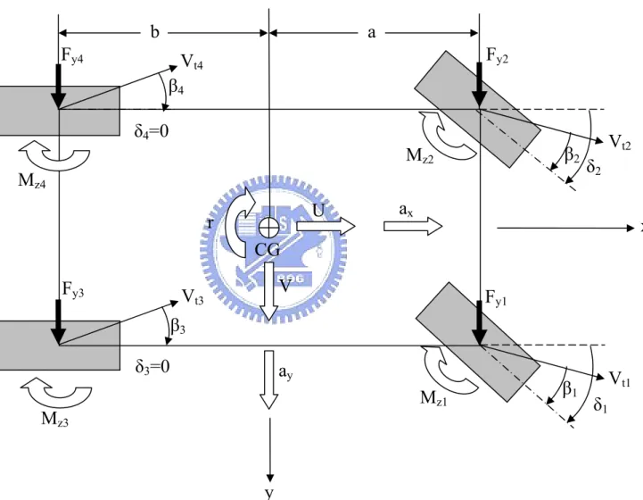
(18) External forces and moments include the force (or the moment) of air resistance, the force (or the moment) of gravity, and the force (or the moment) of wheels acting on the vehicle. We must calculate these forces and moments, apply them in the dynamic differential equations of vehicles, calculate the equations and integration. Thus, we would obtain three degrees of freedom of operation model of vehicles as follow: X = the longitudinal displacement of the car’s center of mass Y = the lateral displacement of the car’s center of mass Ψ = the yaw angle of the vehicle. 2.3 Wheel models of vehicles The main purpose of the wheel mode is to calculate each vehicle wheel’s longitudinal force, lateral force, and aligning torque, which are the function of the parameters, such as sideslip angle, normal force, inclination angle, and traction or braking acceleration.. 2.3.1 Calculate the slip angle β i for each wheel From the longitudinal velocity, the lateral velocity and the yaw angle velocity of the center of mass for the vehicle, as shown in Figure 2.1, we would figure out: the velocity vector of the right-front wheel, T Vx1 = U − f × r ， Vy1 = V + a × r 2. the velocity vector of the left-front wheel, T Vx 2 = U + f × r ， Vy 2 = V + a × r 2 8. (2-4a). (2-4b).

(19) the velocity vector of the right-rear wheel, T Vx 3 = U − r × r ， Vy 3 = V − b × r 2. (2-4c). and the velocity vector of the right-rear wheel. T Vx 4 = U + r × r ， Vy 4 = V − b × r 2. Vti = Vxi 2 + Vyi 2. V xi =. Vxi Vti. V yi =. (2-4d). Vyi Vti. Then comes the equation,. ⎡ V xi × sin δ i − V yi × cos δ i β i = Tan −1 ⎢⎢ ⎢⎣ 1 − V xi × sin δ i − V yi × cos δ i. (. ). ⎤ ⎥ 2 ⎥ ⎥⎦. (2-5). 2.3.2 Calculate the angle of inclination γ i for each wheel The angle of inclination for each wheel can be obtained by the equation (2-6).. γ i = φu + φs / u × γ f. (2-6). 2.3.3 Torque on the drive wheels The torque transmission starts from engine torque, clutch, gearbox, transmission shaft, differential mechanism, wheel axle, to wheels. Here come some factors that affect the torque among vehicle wheels, which are accelerating or braking acceleration a′x produced by the driver, the drive design (either driven by front wheels, rear wheels, or four wheels), and the feature of braking system on the vehicle (the coefficient of braking equation, Q0 and Q1 ) If the 9.

(20) acceleration a′x is positive, the car is braking, while negative, accelerating. The factor to dispose torque can be defined by these conditions as follows: (1) If a′x < 0 (accelerating), cars driven by front wheels, Q = 1. (2) If a′x < 0 (accelerating), cars driven by rear wheels, Q = 0. (3) If a′x < 0 (accelerating), cars driven by four wheels, Q = Wd4. (4) If 0 ≦ a′x ≦ 0.3g (middle braking), Q = Q0 . (5) If a′x > 0.3g (heavy braking), Q = Q0 + Q1 ( a′x − 0.3) .. After figuring out the factor to dispose torque, through the accelerating or braking acceleration a′x , we can obtain braking force or accelerating force for each wheel by equation as follow,. 1 Fx′1 = Fx′2 = × m × a′x × g × Q 2 1 Fx′3 = Fx′4 = × m × a′x × g × (1 − Q ) 2. (2-7a) (2-7b). 2.3.4 Calculate t the normal force for each wheel Whether a car is accelerating at longitudinal vector or lateral vector, the inertia force will differentiate each wheel’s vertical reaction. The variation of vertical reaction of wheels is called lateral weight transfer, caused by the lateral acceleration when the car is turning. The variation of vertical reaction of wheels is called longitudinal weight transfer, caused by the longitudinal acceleration when the car is braking or accelerating. We have the equations of actual lateral and longitudinal acceleration as follows: 10.

(21) •. ay = V + U × r. (2-8). •. ax = U − V × r. (2-9). The following factors affect the amount and distribution of lateral weight transfer. 1. the body of the car rolling, 2. the high variation of the rolling center, and 3. the mass which isn’t supported by springs. The mass not supported by springs.. Here come some equations from which we calculate the amount of lateral weight transfer of the front and rear wheels when vehicles are rolling. WBF = KRdist ×. (a. y. × ms − Fya ) × H ra × cos φs / u − M xa − ms × g × H ra × sin φs / u Tf. WBF = (1 − KRdist ) ×. (a. y. (2-10a). × ms − Fya ) × H ra × cos φs / u − M xa − ms × g × H ra × sin φs / u Tf (2-10b). The amount of the lateral weight transfer of the front and rear wheels is caused by the high variation of the car’s rolling center. Related equations are as follows. WRF =. WRR =. (a. y. × ms − Fya ) × b × RC f. (2-11a). L × Tf. (a. y. × ms − Fya ) × a × RCr. (2-11b). L × Tr. 11.

(22) The amount of the lateral weight transfer of the front and rear wheels is caused by the mass, not supported by springs. Related equations are as follow.. WUF = a y × muf ×. H uf. WUR = a y × mur ×. H ur Tr. (2-12a). Tf. (2-12b). The total amount of the lateral weight transfer of the front and rear wheels is the grand total of the three variations above. WTF = WBF + WRF + WUF. (2-13a). WTR = WBR + WRR + WUR. (2-13b). Since we get the lateral weight transfer, we can calculate the normal force of each wheel with the following equations. Fxa × H sm + Fza × b − M ya m × H sm + muf × H uf + mur × H ur ⎤ m ×b ⎞ 1 ⎡⎛ + ax × s Fz1 = ⎢⎜ muf + s ⎟× g + ⎥ − WTF L ⎠ L L 2 ⎣⎝ ⎦. (2-14a) Fxa × H sm + Fza × b − M ya m × H sm + muf × H uf + mur × H ur ⎤ m ×b ⎞ 1 ⎡⎛ + ax × s Fz 2 = ⎢⎜ muf + s ⎟× g + ⎥ + WTF L ⎠ L L 2 ⎣⎝ ⎦. (2-14b) Fxa × H sm + Fza × b − M ya m × H sm + muf × H uf + mur × H ur ⎤ m ×b ⎞ 1 ⎡⎛ + ax × s Fz 3 = ⎢⎜ muf + s ⎟× g + ⎥ − WTR L ⎠ L L 2 ⎣⎝ ⎦. (2-14c) Fxa × H sm + Fza × b − M ya m × H sm + muf × H uf + mur × H ur ⎤ m ×b ⎞ 1 ⎡⎛ + ax × s Fz 4 = ⎢⎜ muf + s ⎟× g + ⎥ + WTR L ⎠ L L 2 ⎣⎝ ⎦. (2-14d). 12.

(23) 2.3.5 Calculate the coefficient of friction of vehicle wheels’ After each wheel’s vertical reaction, affected by the longitudinal and lateral weight transfer, is figured out, the coefficient of friction can be calculated. The peak of longitudinal friction coefficient µ xpi for wheels can be figured out with the following equation (2-15).. µ xpi = 0.01 × SN × ( P0 + P1 × Fzi + P2 × Fzi2 ). (2-15). The coefficient µ xsi of sliding friction of wheels can be figured out with the following equation (2-16).. µ xsi = 0.01 × SN × ( S0 + S1 × Fzi + S2 × Fzi2 ). (2-16). The lateral slip ratio S pi of wheels can be figured out with the following equation (2-17), when the car braking. S pi = − R0 − R1 × Fzi. (2-17). The peak lateral friction µ yi of wheels can be calculated with the following equation (2-18).. µ yi = 0.01 × SN × ( B3 + B1 × Fzi + B4 × Fzi2 ). 13. (2-18).

(24) 2.3.6 Calculate the maximum allowable longitudinal force generated by wheels With the known coefficient of friction of wheels, we can calculate the maximum of allowable longitudinal and that of lateral forces generated by wheels. Without cars braking/accelerating, Fymax means the maximum of allowable lateral forces generated by wheels, as what are shown in the following. Fy. max. = µ yi × Fzi. (2-19a). Fx. max. = µ xpi × Fzi. (2-19b). If the braking/accelerating force and the centripetal force exist at the same time, we can calculate the maximum of allowable longitudinal force F’xmax with the following equations. (1) If Fy. max. < Fx. max. , the equation to calculate the eccentricity of an ellipse will. Fx2 max − Fy2 max. be ζ =. Fx. , and the equation for the maximum of allowable. max. longitudinal force F’xmax will be Fx′. max. (2) If Fy be ζ =. =. max. cos β i × Fx. max. × (1 − ζ 2 ). (2-20a). 1 − ζ × cos β i. > Fx. max. , the equation to calculate the eccentricity of an ellipse will. Fy2 max − Fx2 max Fy. , and the equation for the maximum of allowable. max. longitudinal force F’xmax will be 14.

(25) Fx′. max. =. cos β i × Fy. max. × (1 − ζ 2 ). (2-20b). 1 − ζ × cos β i. At this time, the main shaft of an ellipse is the longitudinal axis of a wheel.. 2.3.7 Calculate t the longitudinal coefficient of friction µ xi and slip ratio S i for each wheel If the driver needs greater braking force ( Fxi′ ) than the maximum of braking force ( Fx′max ) generated by wheels, the wheels will be locked. Meanwhile, the value of slip ratio on the wheel will be 1( Si = 1 ). If the driver needs greater accelerating force ( Fxi′ ) than the maximum of accelerating force ( Fx′max ) generated by wheels, the wheels will slip. Meanwhile, the value of slip ratio on the wheel will be -1 ( Si = −1 ). Under the conditions when the wheels are lock or slip ( Si = 1 or Si = −1 ), the related equation to figure the longitudinal coefficient of friction of each wheel is as follows.. µ xi = µ xsi × Sgn ( Fxi′ ). (2-21). We can figure the slip ratio S i of wheels with the following equation. +1, if a′x > 0. Si = Sgn ( a′x ) =. 0, if a′x = 0. -1, if a′x < 0. 15.

(26) If the driver need smaller braking or accelerating force Fxi′ than the maximum of braking or accelerating force Fx′max generated by wheels, which means that the wheels are able to generate the braking or accelerating force the driver needs, in normal condition, the equation to figure the longitudinal coefficient of friction of each wheel is as follow.. µ xi =. Fxi′ Fzi. (2-22). 2.3.8 Calculate the longitudinal force Fci for each wheel With the known longitudinal coefficient of friction, we will calculate the longitudinal force under the two condition as follows. 1. When a′x ≦ 0, Fci = µ xi × Fzi 2. When a′x > 0, Fci =. Besides, ρ s =. (2-23a). µ yi × Fzi × Sgn ( ρ s ) tan 2 β i +. (2-23b). 1. ρ s2. µ xi µ yi. 2.3.9 Calculate the lateral force Fsi for each wheel With the known longitudinal force, before we figure the lateral force with equations depending on the following conditions, we must define ε =. 1. ρ s2. .. 1. If the wheels turn freely, neither being locked nor being slipping (Si = 0), the 16.

(27) lateral force can be figured out with the following equation.. Fsi = µ yi2 × Fzi2 − ε × Fci2. (2-24). 2. If the wheels are locked because of the braking moment overloaded (Si = 1), the lateral and longitudinal forces can be figured out with the following equations. Fci = µ xsi × Fzi × cos β i. (2-25a). Fsi = µ xsi × Fzi × sin β i. (2-25b). 3. If the wheels slip because of the accelerating moment overloaded (Si = -1), the lateral and longitudinal forces can be figured out with the following equations. Fci = − µ xsi × Fzi. (2-26a). Fsi = 0. (2-26b). 2.3.10 Coordinate system transformations We can transform the lateral and longitudinal forces from the wheel’s coordinate system into the vehicle’s coordinate system: Fxi = − Sgn (Vxi × cos δ i + Vyi × sin δ i ) × Fci × cos δ i − Fsi × sin δ i. (2-27a). Fyi = − Sgn (Vxi × cos δ i + Vyi × sin δ i ) × Fci × sin δ i − Fsi × cos δ i. (2-27b). With the functions of the normal forces, the lateral forces, and the angle of inclination, aligning torque could be figured out with the equation (2-27c), as 17.

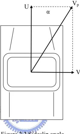
(28) follows: M zi = K1 × Fzi × Fyi − K 2 × Fyi × Fyi +. K 3 × Fzi × γ i. (2-27c). γi. If the wheels are locked or slip because of the braking or accelerating moment overloaded (Si = 1 or Si = -1), the aligning torque is zero (Mzi = 0).. 2.4 Aerodynamic model of a vehicle Aerodynamic forces and moments acting on a vehicle are the functions that include longitudinal velocity, lateral velocity, yaw angle velocity, aerodynamic coefficient, and sideslip angle. The sideslip angle could be figured out from longitudinal velocity and lateral velocity, with the equation as follows:. α = tan −1. V U. (2-28). With the known sideslip angle, the aerodynamic forces and moments acting on a vehicle can be figured out with the following equations: 1. Aerodynamic drag force: Fxa = −0.5 × ρ × U 2 × S front × C xa × Sgn (U ). (2-29a). 2. Aerodynamic lateral force: Fya = −0.5 × ρ × VP2 × S front × C ya × α ,. −. Fya = −0.5 × ρ × VP2 × S front × C ya × (π − α ) ,. π 2. <α <. α≥. π 2. Fya = −0.5 × ρ × VP2 × S front × C ya × ( −π − α ) , α ≤ −. 18. π 2 (2-29b). π 2.

(29) 3. Aerodynamic yawing moment: •. M za = 0.5 × ρ × VP2 × S front × H char × Cna × sin ( 2α ) − Cad × r. (2-29c). 2.5 Dynamic equations of operation model Apply the foregoing aerodynamic forces/moments and forces/moments of wheels into the dynamic differential equations. The acceleration of each degree-of-freedom can be figured out with the following equations. 4. ∑F. •. U=. xi. i =1. m 4. •. V=. •. r=. + Fxa. ∑F i =1. yi. + Fya. m. +V × r. (2-30a). −U × r. (2-30b). a × ( Fy1 + Fy 2 ) − b × ( Fy 3 + Fy 4 ) +. 4 Tf T ( Fx 2 − Fx1 ) + r ( Fx 4 − Fx3 ) + ∑ M zi + M za 2 2 i =1 I zz. (2-30c) Then, integrate the acceleration of each degree-of-freedom to get the velocity. The related equation is as follows: t. •. U = ∫ Udt + U 0. (2-31a). 0. t •. V = ∫ Vdt. (2-31b). 0. t •. r = ∫ rdt. (2-31c). 0. At last, the displacement can be figured out by integrating the velocity of 19.

(30) each degree-of-freedom, with the related equations as follows. t. X = ∫ (U × cos Ψ − V × sin Ψ )dt. (2-32a). 0. t. Y = ∫ (U × sin Ψ + V × cos Ψ )dt. (2-32b). 0. t. Ψ = ∫ rdt. (2-32c). 0. At t = 0, V = r = X = Y = Ψ = 0, and U = U0.. 20.

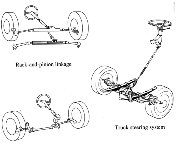
(31) Chapter 3. Force Feedback System. 3.1 The Steering System. 3.1.1 Introduction of the Steering System The design of the steering system has an influence on the direction response behavior of a motor vehicle that is often not fully appreciated. The function of the steering system is to steer the front wheels response to driver command inputs in order to provide overall directional control of the vehicle. However, the actual steer angle achieved are modified by the geometry of the suspension system, the geometry and reactions within the steering system, and in the case of front-wheel-drive (FWD), the geometry and reactions from the drive train. These phenomena will be examined in this section first as a general analysis of a steering system and then by considering the influence of front- wheel-drive.. 3.1.2 The steering linkages The steering system used on motor vehicles vary widely in design [12, 13, 14], but are functionally quite similar. Figure 3.1 illustrate some of these. The steering wheel connects by shaft, universal joints, and vibration isolators to the steering gearbox whose purpose is to transform the rotary motion of the steering wheel to a translational motion appropriate for steering the wheels. The rack-and-pinion system consists of a linearly moving rack and pinion, mounted on the firewall or a forward cross member, which steers the left and right wheels directly by a tie-rod connection. The tie-rod linkage connects to 21.

(32) steering arms on the wheels, thereby controlling the steer angle. With the tie-rod located ahead of the wheel center, as shown in Figure 3.1, it is a forward-steer configuration. The steering gear box is an alternative design used on passenger cars and light trucks. It differs from the rack-and-pinion in that a frame-mounted steering gearbox rotates a pitman arm which controls the steer angle of the left and right wheels through a series of relay linkages and tie rods, the specific configuration of which varies from vehicle to vehicle. A rear-steer configuration is show in the figure, identified by the fact that the tie-rod linkage connects to the steering arm behind the wheel center. Between these two, the rack-and-pinion system has been growing in popularity for passenger cars because of the obvious advantage of reduced complexity,. easier. accommodation. of. front-wheel-drive. systems,. and. adaptability to vehicle without frames. The primary functional difference in the steering systems used on heavy truck is the fact that the frame-mounted steering gearbox steers the left road wheel through a longitudinal drag line, and the right wheel is steered from the left wheel via a tie-rod linkage [12]. The gearbox is the primary means for numerical reduction between the rotational input from the steering wheel and the rotational output about the steer axis. The steering wheel to road wheel angle ratios normally vary with angle, but have nominal values on the order of 15 to 1 in passenger cars, and up to as much as 36 to 1 with some heavy trucks. Initially all rack-and-pinion gearboxes had a fixed gear ratio, in which case any variation in ratio with steer angle was achieved through the geometry of the linkages. Today, rack-and-pinion systems are available that vary their gear ratio directly with steer angle.. 22.

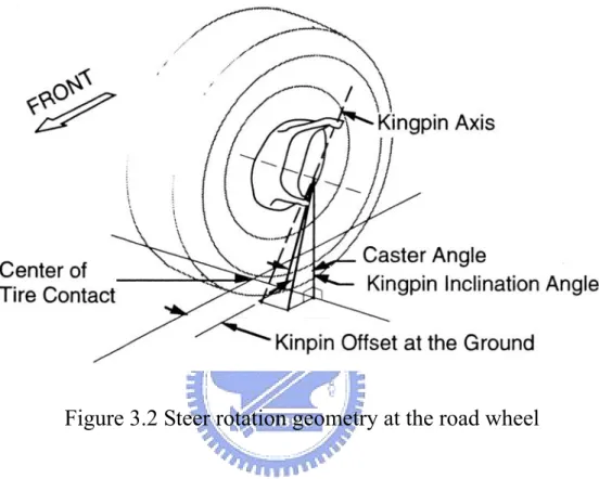
(33) 3.2 Geometry. 3.2.1 Front Wheel Geometry The important elements of a steering system consist not only of the visible linkages just described, but also the geometry associated with the steer rotation axis at the road wheel. The geometry determines the force and moment reaction in the steering system, affecting its overall performance. The important features of the geometry are shown in Figure 3.2. The steer angle is achieved by rotation of the wheel about a steer rotation axis. Historically, this axis has the name “kingpin” axis, although it may be established by ball joint or the upper mounting bearing on a strut. The axis is normally not vertical, but may be tipped outward at the bottom, producing a lateral inclination angle (kingpin inclination angle) in the range of 10-15degrees on passenger cars. It is common for the wheel to be offset laterally from the point where the steer rotation axis intersects the ground. The lateral distance from the ground intercept to the wheel centerline is the offset at the ground and is considered positive when the wheel is outboard of the ground intercept. Offset may be necessary to obtain packaging space for brakes, suspension, and steering components. At the same time, it adds “feel of the road” and reduces static steering efforts by allowing the tire to roll around an arc when it is turned [15]. Caster angle result when the steer rotation axis is inclined in the longitudinal plane. Positive caster places the ground intercept of the steer axis ahead of the center of tire contact. A similar effect is created by including a longitudinal offset between the steer axis and the spin axis of the wheel, 23.

(34) although this is only infrequently used. Caster angle normally ranges from 0 to 5 degrees and may vary with suspension deflection.. 3.2.2 Formulation of Geometry Before we analyze the geometry, we define the geometry meaning of each term in fundamental dynamics equation.. Nomenclature. d: kingpin offset at the ground Fxr: tractive force on right-front wheel Fxl: tractive force on left-front wheel Fyr: lateral force on right-front wheel Fyl: lateral force on left-front wheel Fzr: vertical force on right-front wheel Fzl: vertical force on left-front wheel Ffeedback: feedback force on the steering wheel Mzr: aligning torque on right-front wheel Mzl: aligning torque on left-front wheel MT: moment produced by tractive force ML: moment produced by lateral force MV:. moment produced by vertical force. MV,inclination: moment produced by vertical force acting on lateral inclination angle MV,caster: moment produced by vertical force acting on caster angle MAT:. moment produced by aligning torque 24.

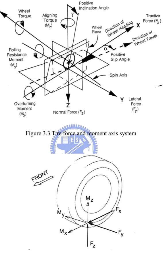
(35) MALL: the total moment r: tire radius Rw: steering wheel radius λ: lateral inclination angle υ: caster angle δ: steer angle τ: gear ratio. 3.3 Steering System Forces and Moments The forces and moments imposed on the steering system emanate from those generated at the tire-road interface. The SAE has selected a convention by which to describe the force on a tire, as shown in Figure 3.3. Assume that the forces are measured at the center of the contact with the ground and provide a convenient basis by which to analyze steering reactions. The ground reactions on the tire are described by three forces and moments, as follow: 1. Normal force 2. Tractive force 3. Lateral force 4. Aligning torque 5. Rolling resistance 6. Overturning moment. The reaction in the steering system is described by the moment produced on the steer axis, which must be resisted to control the wheel steer angle. 25.

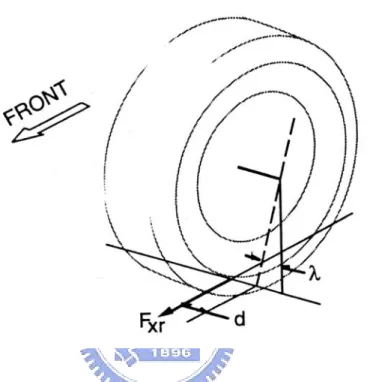
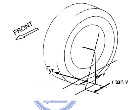
(36) Ultimately, the sum of moments from the left and right wheels acting through the steering linkages with their associated ratios and efficiencies account for the steering-wheel torque feedback to the driver. Figure 3.4 shows the three forces and moments acting on a right-hand road wheel. Each will be examined separately to illustrate its effect on the steering system.. 3.3.1 Tractive Force The tractive force, Fx, acts on the kingpin offset to produce a moment as shown in Figure 3.5. Then net moment is: M T = (Fxl − Fxr ) ⋅ d. (3-1). The left and right moments are opposite in direction and tend to balance through the relay linkage. Imbalances, such as may occur with a tire blowout, brake malfunction, or split coefficient surfaces, will tend to produce a steering moment which is dependent on the lateral offset dimension.. 3.3.2 Lateral Force The lateral force, Fy, acting at the tire center produces a moment through the longitudinal offset resulting from caster angle, as shown in Figure 3.6. The net moment produced is: M L = (Fyl + Fyr ) ⋅ r tanν. (3-2). 26.

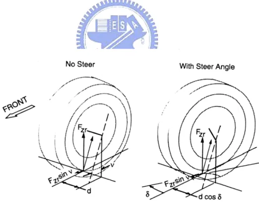
(37) The lateral force is generally dependent on the steer angle and cornering condition, and with positive caster produces a moment attempting to steer the vehicle out of the turn.. 3.3.3 Vertical Force The vertical force acting on lateral inclination angle, illustrated in Figure 3.7, results in a sine angle force component, which normally acts lateral on the moment arm when the wheel is steered. The moment is zero at zero steer angle. When steering, both sides of the vehicle lift, an effect which is often described as the source of the centering moment. M V ,inclination = −(Fzl + Fzr ) ⋅ d ⋅ sin λ ⋅ sin δ. (3-3). The caster angle results in a sin angle force component, which nominally acts forward on the moment arm as shown in Figure 3.8. M V ,caster = (Fzl − Fzr ) ⋅ d ⋅ sinν ⋅ cos δ. (3-4). Then the net moment produced by vertical force is: M V = (Fzl − Fzr ) ⋅ d ⋅ sinν ⋅ cos δ − (Fzl + Fzr ) ⋅ d ⋅ sin λ ⋅ sin δ. (3-5). When steer angle, one side of the axle lift and the other drops, so that the net moment produce depends also on the roll stiffness of the front suspension as it influences the left and right wheel roads.. 27.

(38) 3.3.4 Aligning Torque The aligning torque, M, acts vertically and may be resolved into a component acting parallel to the steering axis. Since moments may be translated without a change in magnitude, the equation for the net moment is: M. AT. =M. zl. + M zr. (3-6). Under normal driving conditions, the aligning torques always act to resist any turning motion, thus their effect is under steer. Only under high braking conditions do they act in a contrary fashion.. 3.3.5 Rolling Resistance and Overturning Moments These moments at most only have a sine angle component acting about the steer axis. They are second-order effects and are usually neglected in analysis of steering system torques.. 3.4 Force Feedback On The Steering Wheel These equations, (3-1), (3-2), (3-5), (3-6), are the moments of steering axis, we can add direct them to get the total moment, MALL, on the kingpin axis: M. ALL. ). (. cos λ 2 + ν 2 = M +M +M +M T L V AT. (3-7). Then we can through the steering system model, as shown Figure 3.9, and calculate the force on the steering wheel by the way of the total moment. However, in our simulation, in order to simplify our analysis and retrench the time to calculate, we usually neglect the rigidity of the steering linkage, K, and 28.

(39) other coefficient of viscosity, and the total moment divides gear ratio to get the torque on the steering wheel. Then the torque on the steering wheel divides the radius of the steering wheel to get the force which driver sustains.. F. feedback. =. M. ALL ⋅ 1 R τ w. (3-8). 29.

(40) Chapter 4. Hardware Integration. 4.1 Hardware Structure The hardware of the steering wheel system is mainly divided into four parts, a principal mechanism, driving device, angular potential meter, and signal process interface. We use the principle of dc motor controllable system, as figure 4-1, to make the force feedback steering wheel output appropriate forces accurately at real-time. In this chapter, we will describe each device in the steering wheel system and analyze the control principle.. 4.2 Principal Mechanism In figure 4-2, it’s a mechanism of the steering wheel which we design with Internet Motion Navigator Corp. during education and industry cooperation. In the mechanism, we can know the torque produced by motor allows a pulley whose ratio of radius is 3:1 to drive the steering wheel on another axis. It indirectly brings forces for users to achieve the force feedback effects produced in virtual reality. At the same time, we add a mechanism on the front of the pulley to limit rotational angle, and then we can ward off the potential meter breakdown because of rotating over-angle.. 4.3 Driving Device Because the driving device in the force feedback steering wheel needs accurate and stable output torques, we use a dc motor device and combine a PWM motor driver to control output current. 30.

(41) 4.3.1 DC Motor We use a geared motor produced by SHAYANG YE Industrial Co., Ltd. in this system, as figure 4-3, and its specification is shown in table 4-1. According to the specification, we know that the rated torque is 0.5 Nm, from which we can find the maximum force feedback to users from the mechanism of steering wheel. The given radius of steering wheel is 20 mm (0.2 m) and the ratio of the pulley’s radius is 3. From the equation below (4-1), Feedback Force(N) =. Output Torque(N/m) × Ratio of Pulley's Radius Radius of Steering Wheel(m). (4-1). We know that the maximum force feedback to users is 7.5 N (alike 0.77 kg).. 4.3.2 PWM Motor Driver We use the chip, A3953S as figure 4-4, designed for bidirectional pulse-width modulated (PWM) current control of inductive loads and produced by Allegro Microsystems. We can know the features of the chip as follow: z. ±1.3 A Continuous Output Current. z 50 V Output Voltage Rating z 3 V to 5.5 V Logic Supply Voltage z Internal PWM Current Control z Saturated Sink Drivers (Below 1 A) z Fast and Slow Current-Decay Modes z Automotive Capable z Sleep (Low Current Consumption) Mode z Internal Transient-Suppression Diodes z Internal Thermal-Shutdown Circuitry 31.

(42) z Crossover-Current and UVLO Protection. In dc motor applications, which require accurate positioning at low or zero speed, PWM of the PHASE input is selected typically. This simplifies the servo control loop because the transfer function between the duty cycle on the PHASE input and the average voltage applied to the motor is more linear than in the case of ENABLE PWM control (which produces a discontinuous current at low current levels).With bidirectional dc servo motors, the PHASE terminal can be used for mechanical direction control. Similar to when braking the motor dynamically, abrupt changes in the direction of a rotating motor produces a current generated by the back-EMF. The current generated will depend on the mode of operation. If the internal current control circuitry is not being used, then the maximum load current generated can be approximated by I LOAD =. (VBEMF + VBB ) R LOAD. (4-2). where VBEMF is proportional to the motor’s speed. If the internal slow current-decay control circuitry is used, then the maximum load current generated can be approximated by I LOAD =. VBEMF R LOAD. (4-3). 4.4 Angular Potential Meter By means of angular potential meter, we can obtain the angle rotated by steering wheel. The angle is also the steering angle of the wheel. This angular 32.

(43) potential meter outputs different voltage with different rotational angle. We can know the steering angle of steering wheel by the output voltage [16]. See figure 4-5.. 4.5 Signal Process Interface ST72F651 is the chip processing all signals in the steering wheel system and produced by STMicroelectronics, as figure 4-6. We use some features on ST72F651 as follow: z USB (Universal Serial Bus) Interface. z Full speed bulk applications. z 47 programmable I/O ports. z PWM/BRM Generator (with 2 10-bit PWM/BRM outputs). z 8-bit A/D Converter (ADC) with 8 channels. z PLL for generating 48 MHz USB clock using a 12 MHz crystal.. This PWM/BRM peripheral includes a 6-bit Pulse Width Modulator (PWM) and a 4-bit Binary Rate Multiplier (BRM) Generator. It allows the digital to analog conversion (DAC) when used with external filtering. The 10 bits of the 10-bit PWM/BRM are distributed as 6 PWM bits and 4 BRM bits. The generator consists of a 10-bit counter (common for all channels), a comparator and the PWM/BRM generation logic. The on-chip Analog to Digital Converter (ADC) peripheral is a 8-bit, successive approximation converter with internal sample and hold circuitry. This peripheral has up to 8 multiplexed analog input channels (refer to device pin out description) that allow the peripheral to convert the analog voltage levels from 33.

(44) up to 8 different sources. In software, we program DirectX 8.0 SDK to operate ST72F651. The Direct Input Interface Library is designed to allow programmers to utilize a force feedback joystick without knowing how to program DirectX. It contains the necessary functions for accessing the positions of the various buttons, switches, and levers as well as communicating with the servo motors to provide constant, directional and periodic, vibrating forces.. 4.6 Armature control of dc motors Consider the armature-control dc motors shown in figure 4.7, where the field current is held constant [17]. In this system, R = armature resistance, L = armature inductance, i = armature current, i = field current, e = applied armature voltage, e = back electromotive force, θ = angular displacement of the motor shaft,. T = torque developed by the motor, J = equivalent moment of inertia of the motor and load, b = equivalent viscous-friction coefficient of the motor and load. The torque T developed by the motor is proportional to the armature current i. T = KT × ia. (4-4). 34.

(45) where KT is a motor-torque coefficient. When the armature is rotating, a voltage proportional to the product of the flux and angular velocity is induced in the armature. For a constant flux, the induced voltage eb is directly proportional to the angular velocity eb = K b. dθ dt. dθ , or dt (4-5). Where eb is the back electromotive force and K b is a back electromotive force coefficient. The speed of armature-controlled dc motor is controlled by the armature voltage ea . The differential equation for the armature circuit is La. dia + Raia + eb = ea dt. (4-6). The armature current produces the torque that is applied to the inertia and friction, so d 2θ dθ = T = KT ia J 2 +b dt dt. (4-7). Assuming that all inertia conditions are zero, and taking the Laplace transforms of equations (4-5), (4-6), (4-7). We obtain the following equations: K b sθ ( s ) = Eb ( s ). (4-8). ( La s + Ra ) I a ( s ) + Eb ( s ) = Ea ( s ). (4-9). ( Js 2 + bs)θ ( s) = T ( s) = KT I a ( s). (4-10). 35.

(46) Considering Ea ( s ) as the input and T ( s) as the output, it is possible to construct a block diagram from equations (4-8), (4-9), and (4-10). See figure 4.8. The armature-controlled dc motor is a feed back system. The transfer function for the dc motor considered here is obtained as. G ( s) =. θ ( s) E ( s). =. K T s(( La s + Ra )( Js + b) + K K ) T b. (4-11). The inductance La in the armature circuit is small and may be neglected. If La is neglected and b is zero, then the transfer function given by equation (4-11) reduce to. θ (s) Ea ( s ). =. KT Ra Js + KT K b s. (4-12). 2. If we know the output torque we want and parameters ( J , Ra , KT , and K b ), we can obtain the input voltage form equation (4-12).. 36.

(47) Chapter 5. Conclusion. Many force feedback joysticks are sold in the business situation, and Logitech’s is the most popular one now. Here we would like to compare the force feedback steering wheel that we designed with Logitech’s force feedback joystick. Firstly, as for the software, we calculate proper forces with correct physical reasoning. On the contrary, Logitech’s joystick presents constant forces. Secondly, as far as hardware is concerned, we use the chip, ST72F651, in signal process interface, and we can know that ST72F651 is USB interface and has full-speed (12 Mb/s) bulk applications. The most important feature of ST72f651 is that it has A/D converter with 8 channels, D/A converter with 2 channels, and more digital input or output channels. Logitech’s joystick also uses USB interface, but with low-speed transmission and without output ports. Although our force feedback steering wheel has many advantages, there are still some flaws in mechanism and dc motor. In the future, we will improve the mechanism of steering wheel to reduce the cost, and investigate brushless dc motors.. 37.

(48) References [1] Pimental, K. and K. Teixeira, “Virtual Reality: Through the New Looking Glass”, second edition, Windcrest McGraw-Hill, New York, 1994. [2] Krueger, M., “Artificial Reality II”, Addison-Wesley, Menlo Park, CA, 1991. [3] Burdea, G. and P. Coiffet, “Virtual Reality Technology”, John Wiley & Sons, New York City, June, 1994. [4] Akka, R., “Utilizing 6D head-tracking data for stereoscopic computer graphics perspective transformations”, StereoGraphics Co., San Rafael, CA, 8pp, 1992. [5] Wenzel, E., “Localization in Virtual Acoustic Display”, Presence-Teleoperators and Virtual Environments, Vol. 1,No. 1, MIT Press, pp. 80-107, October, 1992. [6] Wenzel, E., “Launching Sounds Into Space”, Proceedings of Cyberarts Conference, Miller Freeman, Inc., San Francisco, pp. 87-93, October, 1992. [7] Burdea, G., J. Zhuang, E. Roskos, D. Silver and N. Langrana, “A Portable Dextrous Master with Force Feedback”, Presence-Teleoperators and Virtual Environments, Vol. 1,No. 1, MIT Press, Cambridge, MA, pp. 18-27, March, 1992. [8] Marcus, B., “Sensing, Perception and Feedback for VR”, VR System Fall 93 Conference, SIG Advanced Applications, New York, 1993. [9] Piantanida, T., D. Boman and J. Gille, “Human Perceptual Issues and Virtual Reality”, Virtual Reality System, Vol. 1, No. 1, pp. 43-52, 1993. [10] Fuchs, H., J. Poulton, J. Eyles, T. Greer, J. Goldfeather, D. Ellsworth, S. Molnar, G. Turk, B. Tebbs, and L. Israel, “Pixel-Planes 5: A Heterogeneous Multiprocessor Graphics System Using Processor-Enhanced Memories”, 38.

(49) Computer Graphics, Vol. 23, No.3, pp. 79-88, July, 1989. [11] Papper M. and M. Gigante, “Using Physical Constraints in a Virtual Environment”, in Virtual Reality System, Academic Press, Orlando, FL, pp. 107-118. [12] Durstine, J.W., “The Truck Steering System from Hand Wheel to Road Wheel”, SAE SP-374, January 1974. [13] Gillespie, T.D., “Front Brake Interaction with Heavy Vehicle Steering and Handling during Braking”, SAE Paper No. 760025, 1976. [14] Dwiggins, B.H., “Automotive Steering Systems”, Delmar Publisher, Albany, NY, 1968. [15] Taborek, J.J., “Mechanics of Vehicles”, Towmotor Corporation, Cleveland, OH, 957. [16] 楊善國編著，感測與量度工程。台北：全華，1994。 [17] 張碩編著，自動控制系統。台北：全華，1998。 [18] Gillespie, T.D., “Fundamentals of Vehicle Dynamics”, Society of Automotive Engineers, 1992. [19] Wong, J.Y., “Theory of Ground Vehicles”, Wiley-Interscience, New York, 1993. [20] Burdea, G.C., “Force and Touch Feedback for Virtual Reality”, John Wiley & Sons, Inc., New York, 1996.. 39.

(50) Figures. Figure 1.1 Schematic diagram of the force feedback system. 40.

(51) Figure 1.2 Schematic block diagram of the force feedback system. 41.

(52) b. a. Fy4. Fy2. Vt4 β4 δ4=0. β2. Mz2 Mz4 U. r. Vt2 δ2. ax. x. CG Fy3. V. Vt3. Fy1. β3 δ3=0. ay Mz1. Mz3. y. Figure 2.1 Operation models of vehicles. 42. β1. Vt1 δ1.

(53) Vp. U. α. V. Figure 2.2 Sideslip angle. 43.

(54) Figure 3.1 Illustration of typical steering systems. 44.

(55) Figure 3.2 Steer rotation geometry at the road wheel. 45.

(56) Figure 3.3 Tire force and moment axis system. Figure 3.4 Forces and moments acting on a right-hand road wheel. 46.

(57) Figure 3.5 Steering moment produced by tractive force. 47.

(58) Figure 3.6 Steering moment produced by lateral force. 48.

(59) Figure 3.7 Moment produced by vertical force acting on lateral inclination angle. Figure 3.8 Moment produced by vertical force acting on caster angle. 49.

(60) Figure 3.9 Steering linkages model. 50.

(61) Virtual Reality. D/A convector. Motor Driver. A/D convector. DC Motor. Potential Meter. Figure 4.1 Hardware Integration of steering wheel system. 51. Steering Wheel.

(62) Figure 4.2 Mechanism of the steering wheel. 52.

(63) Figure 4.3 dc motor. Figure 4.4 A3953S. 53.

(64) Figure 4.5 Angular Potential Meter. Figure 4.6 ST72F651. 54.

(65) ea. eb. θ. J. T. ia if = constant. b. Figure 4.7 Armature-Control dc motors. Ea(s). +. 1. Ia(s). Las+Ra. KT. T(s). •. θ (s). 1 Js+b. Eb(s) Kb. s. Figure 4.8 block diagram. 55. 1 s. θ (s).

(66) Tables. Motor specification. value. unit. rated torque. 0.5. Nm. torque constant. 0.5556. Nm/A. rated revolution. 190. RPM. rated current. 0.9. A. maximum voltage. 24. Volt. Table 4.1 Specification of dc motor. 56.

(67)