利用延伸式有限狀態機來實現介面規格相符驗證之研究

國 立 交 通 大 學

電子工程學系電子研究所

博 士 論 文

利用延伸式有限狀態機來實現介面規格

相符驗證之研究

Interface Compliance Verification

Using the EFSM Model

研 究 生 ：石哲華

指導教授 ：周景揚 博士

利

利

利用

用

用延

延

延伸

伸

伸式

式

式有

有

有限

限

限狀

狀

狀態

態

態機

機

機來

來

來實

實

實現

現

現

介

介

介面

面

面規

規

規格

格

格相

相

相符

符

符驗

驗

驗證

證

證之

之

之研

研

研究

究

究

學

學

學生

生

生：

：

：石

石

石哲

哲

哲華

華

華

指導

指

指

導

導教

教

教授

授

授：

：

：周

周

周景

景

景揚

揚

揚

國

國

國立

立

立交

交

交通

通

通大

大

大學

學

學

電

電

電機

機

機學

學

學院

院

院 電

電

電子

子

子工

工

工程

程學

程

學

學系

系

系 電

電

電子

子

子研

研

研究

究

究所

所

所

摘

摘

摘要

要

要

智產設計是否吻合其傳輸介面，能夠在整合後正確地溝通資料， 便成 為現今系統單晶片驗證上的一大課題。

模擬驗證(simulation-based Verification)是目前最廣泛應用在介面相 容性驗證(interface compliance verification)的方法， 模擬驗證主要是利 用模擬器(simulator)來模仿晶片的實際運作， 具有較低的進入門檻及 可處理較大電路為其優勢。 在模擬驗證中， 驗證人員透過適當的外部 輸入向量(input stimuli)來驅動待驗證設計的內部行為， 同時，觀察模 擬時的訊號變化來檢查是否有違反設計規格的情形， 在一段時間的模 擬之後，涵蓋率量度(coverage metric)則經常被採用來量化當前的驗證 品質。 傳統上運用人力來撰寫輸入向量、比對模擬結果的作法， 不僅 費時耗力也容易出錯， 如果能夠利用工具自動化地完成上述工作，則 可有效地加速模擬驗證的流程。 一 般 的 介 面 規 格 大 多 是 使 用 自 然 語 言(例 如 英 文)或 時 序 示 意 圖(timing diagram)這類非正規的方法來描述， 在驗證自動化的過程 中， 首要任務便是如何將這些介面規格轉譯為定義明確的形式(利用正 規的語言或表示法)。 然而許多正規驗證語言的學習及使用上的難度較 高， 容易導致轉譯過程中的錯誤， 進而影響驗證的正確性。 在這篇 論文中，我們利用了有限狀態機模型的優點， 同時考量介面規格常見 的特性， 發展了兩種基於延伸式有限狀態機模型(Extended Finite State Machine)的介面規格描述方式， 用來系統化地解譯介面規格。

對於介面相容性驗證的問題， 我們提出了一套完整的自動化流 程。 透過所提出之演算法， 我們可以從單一延伸式有限狀態機模 型自動化地產生模擬驗證時所需之各種主要元件： 包含了向量產 生器(stimulus generator)、協定檢查器(protocol checker)及涵蓋率分析 器(coverage analyzer)。 這些元件由於來自同一個模型， 可以避免元件 間的不一致性， 同時，我們的方法也提供了許多便於驗證與除錯的特 性， 可用來大幅提升驗證的效率， 實驗的結果顯示了， 我們的方法 的確可以有效地執行介面規格相容性驗證並縮短所需的時間。

Interface Compliance Verification

Using the EFSM Model

Student: Che-Hua Shih

Advisor: Dr. Jing-Yang Jou

Department of Electronics Engineering

Institute of Electronics

National Chiao Tung University

Abstract

In designing a modern system-on-a-chip (SOC), the platform-based de-sign methodology with reusable intellectual property (IP) cores is usually adopted to accelerate both the design and verification process. In this kind of methodology, an IP core is often wrapped with certain interface logic and integrated into a system platform based on a specific interface protocol. To ensure that an IP core can concordantly communicate with others within the

system, it is very important to guarantee that its interface logic exactly con-forms to the protocol for communication. Hence, interface compliance veri-fication becomes an essential part in the SOC veriveri-fication flow.

The simulation-based approaches are widely-used in interface compli-ance verification works. Simulation-based verification has a lower barrier to entry and can handle large designs. In this kind of approaches, appro-priate input stimuli are applied to trigger the design’s internal operations. Simultaneously, the signal changes are observed to check if there is any vio-lations against the specification. Besides, certain coverage metrics are usually adopted to quantify the verification completeness. Typically, those tasks are made manually which are time-consuming and error-prone. To achieve high verification efficiency, automation is necessary to speed up the verification process.

In general, interface protocol specifications are written with natural lan-guages or timing diagrams. To enable the automatic verification process, the first task is to translate the original specification into a well-defined represen-tation. In this dissertation, we developed two kinds of extended finite state machine (EFSM) models which are suitable for representing common inter-face protocols. Besides, we propose a unified framework using the EFSM model for interface compliance verification. Via the proposed algorithms, the

EFSM model can be automatically translated into a simulation kit consisting of three verification components, a stimulus generator, a protocol checker, and a coverage analyzer. The simulation kit has many useful features to in-crease the verification efficiency. Our experimental results demonstrate that the proposed framework improves not only the performance but also the qual-ity for interface compliance verification.

Acknowledgements

This dissertation would not have been possible to complete without the assistance and support of numerous individuals. First, I would like to express my sincere appreciation to my advisor, Professor Jing-Yang Jou (周 景 揚) for his support, suggestions and guidance throughout my graduate life. And I would also like to thank Professor Juinn-Dar Huang (黃俊達), who had given me a lots of valuable suggestions and discussions.

I would like to thank the members of my dissertation committee, Profes-sor Sy-Yen Kuo (郭斯彥), ProfesProfes-sor Sao-Jie Chen (陳少傑), ProfesProfes-sor Kuen-Jong Lee (李昆忠), Professor Shi-Yu Huang (黃錫瑜), Professor Chau-Chin Su (蘇朝琴), and Professor Chun-Yao Wang (王俊堯), for their comments and suggestions .

Besides, special thanks to Geeng-Wei Lee (李 耿 維), Cheng-Yeh Wang (王成業), Tai-Ying Jiang (江泰盈), Hen-Ming Lin (林恆民), Chia-Chih Yen (顏嘉志), Chien-Hua Chen (陳建華), Bu-Ching Lin (林步青), and all other EDA members for the wonderful time we share together.

My deepest appreciation goes to my wife, Huei-Min Lin (林惠敏), who fills my life with laughter and love. Thank for her patient care on my life and her endless support. Finally, I would like to devote this dissertation and its honor to my parents and family. Thanks for their love and encouragement.

Contents

1.1 Interface Compliance Verification . . . 1

1.2 Stimulus Generation . . . 4

1.3 Correctness Checking . . . 7

1.4 Coverage Analysis . . . 8

1.5 Automatic Simulation Kit Generation . . . 9

1.6 Dissertation Organization . . . 10

2 An Overview of Our Methodology 11 2.1 Different Viewpoints for Interpreting a Specification . . . 11

2.2 The Flow of Our Methodology . . . 13

2.3 Related Works . . . 15

3 GEFSM-Based Framework 19 3.1 The Traditional EFSM Model . . . 20

3.2 The GEFSM Model . . . 21

3.3 An Example Protocol Specification . . . 22

3.4 Stimulus Generation Flow . . . 25

3.5 Stimulus Biasing . . . 30

3.5.1 Transition-level Biasing / Transaction-level Biasing . . . 31

3.5.2 Bit-level biasing / Word-level biasing . . . 32

3.5.3 Feedback for Biasing Refinements . . . 34

3.6 Automatic Translation . . . 35 3.7 Experimental Results . . . 40 3.7.1 Stimulus Biasing . . . 41 3.7.2 Performance Analysis . . . 42 3.7.3 Error Detection . . . 44 3.7.4 Synthesis Results . . . 44 3.8 Summary . . . 45

4 CEFSM-Based Framework 47

4.1 The CEFSM Model . . . 48

4.2 CEFSM-based Correctness Checker . . . 51

4.3 CEFSM-based Stimulus Generator . . . 54

4.4 Automatic Translation . . . 61

4.5 Coverage Metrics . . . 64

4.5.1 The Basic Coverage Metrics . . . 64

4.5.2 The Transaction-level Functional Coverage . . . 65

4.6 Experimental Results . . . 70 4.6.1 Coverage Comparison . . . 71 4.6.2 Stimulus Biasing . . . 74 4.6.3 Error Detection . . . 75 4.6.4 Synthesis Results . . . 76 4.7 Summary . . . 76

5 Conclusions and Future Works 79 5.1 Conclusions . . . 79

5.2 Future Works . . . 80

List of Figures

1.1 The platform-based design methodology. . . 2

1.2 Typical interface compliance verification flow. . . 3

1.3 A typical environment for simulation-based verification. . . 5

2.1 Modeling in different points of view. . . 12

2.2 The overall flow of our verification methodology. . . 14

2.3 The flow of rule-based methodology. . . 16

2.4 The flow of CWL-based methodology. . . 16

3.1 A same protocol in two different FSM representations. . . 21

3.2 A simple transfer of a 4-beat burst. . . 23

3.3 The slave interface of the simplified protocol. . . 23

3.4 A burst with a wait state. . . 24

3.5 A burst with a busy state. . . 25

3.6 The protocol modeling steps with GEFSM. . . 26

3.8 Stimulus generation flow. . . 28

3.9 An example of bit-level biasing. . . 32

3.10 Stimulus generator translation flow. . . 36

3.11 The interface of the stimulus generator. . . 37

3.12 Weighted selection procedure. . . 39

3.13 The block diagram of the proposed GEFSM-based stimulus generator. . . 40

4.1 A CEFSM example. . . 52

4.2 CEFSM to correctness checker. . . 53

4.3 A simulation example. . . 55

4.4 CEFSM to stimulus generator. . . 56

4.5 The operation flow of a constraint producer. . . 58

4.6 Two different kinds of relations. . . 61

List of Tables

2.1 Comparisons among two EFSM models . . . 13

2.2 Comparisons among three approaches . . . 17

3.1 Biasing information I . . . 31

3.2 Biasing information II . . . 35

3.3 Basic information of selected DUVs . . . 41

3.4 Results of word-level biasing . . . 42

3.5 Run-time analysis of different stimulus generators . . . 43

4.1 Coverage comparisons for Case I . . . 73

4.2 Coverage comparisons for Case II . . . 74

4.3 Biasing settings . . . 75

Chapter 1

Introduction

1.1 Interface Compliance Verification

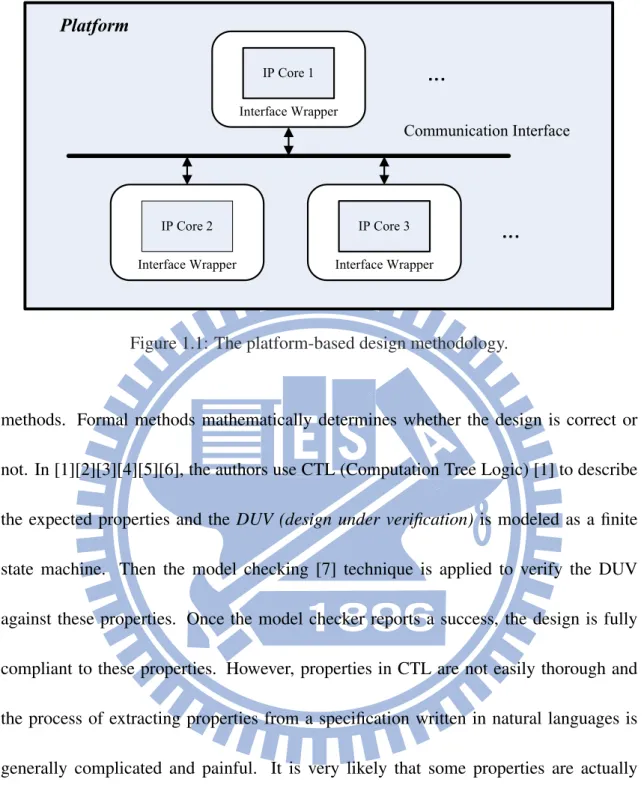
In designing a modern system-on-a-chip (SOC), the platform-based design methodology with reusable intellectual property (IP) cores is usually adopted to accelerate both the de-sign and verification process. Fig. 1.1 illustrates the concept of this methodology. Each pre-verified IP core is wrapped with certain interface logic and integrated into a system platform based on a specific interface protocol. In order to ensure that an IP core can concordantly communicate with others within the system, it is very important to guaran-tee that its interface logic exactly conforms to the protocol for communication. Hence, interface compliance verification becomes an essential part in the SOC verification flow.

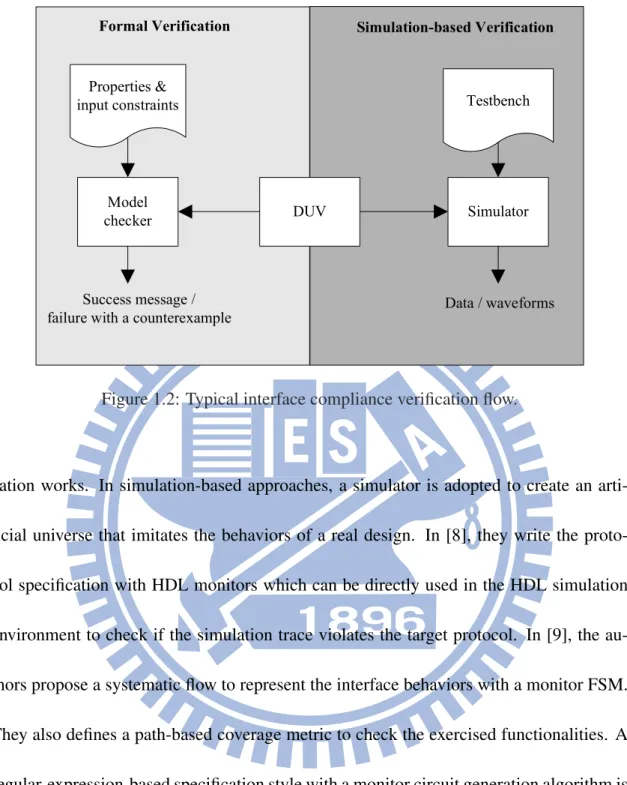
There are two major categories in the field of interface compliance verification: formal methods and simulation-based ones. Fig. 1.2 illustrates the basic concept of these two

Interface Wrapper IP Core 1 Interface Wrapper IP Core 2 Interface Wrapper IP Core 3 Communication Interface Platform

Figure 1.1: The platform-based design methodology.

methods. Formal methods mathematically determines whether the design is correct or not. In [1][2][3][4][5][6], the authors use CTL (Computation Tree Logic) [1] to describe the expected properties and the DUV (design under verification) is modeled as a finite state machine. Then the model checking [7] technique is applied to verify the DUV against these properties. Once the model checker reports a success, the design is fully compliant to these properties. However, properties in CTL are not easily thorough and the process of extracting properties from a specification written in natural languages is generally complicated and painful. It is very likely that some properties are actually implied by the specification but accidentally not extracted and thus ignored during formal verification. Moreover, memory explosion and excessively long runtime may be even serious problems as the design size increases.

verifi-Properties & input constraints Formal Verification Testbench Model checker Simulator Simulation-based Verification Success message / failure with a counterexample

Data / waveforms DUV

Figure 1.2: Typical interface compliance verification flow.

cation works. In simulation-based approaches, a simulator is adopted to create an arti-ficial universe that imitates the behaviors of a real design. In [8], they write the proto-col specification with HDL monitors which can be directly used in the HDL simulation environment to check if the simulation trace violates the target protocol. In [9], the au-thors propose a systematic flow to represent the interface behaviors with a monitor FSM. They also defines a path-based coverage metric to check the exercised functionalities. A regular-expression-based specification style with a monitor circuit generation algorithm is proposed in [10]. Another similar work in [11] generates monitor circuit from GSTE as-sertion graphs. Simulation-based approaches have better scalability against formal ones. However, the simulation-based approaches suffer from long simulation time and the false positive problem. Hence, how to perform simulation-based verification efficiently and

effectively is very import.

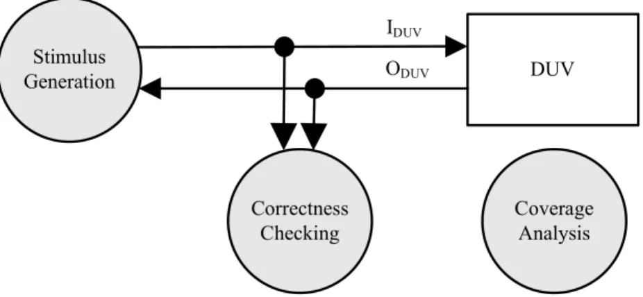
A typical simulation environment for functional verification is shown in Fig. 1.3. The DUV is the verification target. The two directed edges labelled with IDU V and ODU V denote the input and output (I/O) signal sets of the DUV, respectively. Three tasks, the stimulus generation, the correctness checking, and the coverage analysis, are included in the environment. During simulation, the stimulus generation task provides necessary

IDU V values to trigger the DUV’s operations, and the correctness checking task exam-ines the simulation data for error detection. After simulation, the coverage analysis is performed to measure the verification completeness. Each task plays an important role in simulation-based verification, and many techniques have been proposed to fulfill these tasks in the last decades.

1.2 Stimulus Generation

To exercise different operations of a DUV, various input stimuli are required. On the one hand, since the inputs to the DUV must conform to the specification, randomly generated stimuli without any constraints are usually invalid which must be identified, discarded and thus slow down the verification process. Generally, input stimuli are often made manually by the designers who are familiar with the specification. In common interface protocol specifications, stimuli applied to a DUV need to dynamically interact with the DUV’s responses, thus the stimulus generation must be made with extreme cares. On

Correctness Checking Coverage Analysis DUV Stimulus Generation IDUV ODUV

Figure 1.3: A typical environment for simulation-based verification.

the other hand, in order to expose possible design errors of the DUV, a large amount of stimuli are required. However, the manual stimulus development tends to be error-prone and time-consuming. As a result, many research works [12] [13] [14] [15] [16] [17] [18] [19] [20] [21] prefer to build a constraint-based stimulus generator to automate this process. Constraints can be regarded as formal specifications of design behaviors. A constraint-based stimulus generator produces only valid stimuli based on the given constraints. Meanwhile, it is generally not uncommon that multiple valid stimuli exist for a given set of constraints. Some generators pick the first valid one they find while others choose one of the valid stimuli randomly. In general, verification engineers prefer owning more controllability over simulation, thus biasing techniques are often along with the stimulus generation. Biasing allows user-defined settings to increase or decrease the appearance counts of certain stimuli. While constraints limit the random stimuli to valid space, the bias settings can further guide the stimuli to hit the interested design corners.

de-cision diagram (BDD) [24] solvers as their constraint-solving engines. The SAT method is a formal technique that is generally capable of solving a large number of complex con-straints. However, a typical SAT solver often generates only one feasible solution under a given constraint set with no biasing capability. Alternatively, solving constraints with BDDs is relatively easier to be combined with the bit-level biasing approach. However, the weakness of the BDD-based solver is the memory explosion problem while handling a large set of complex constraints.

Yuan et al. [13] propose a general-purpose stimulus generation system, called

Sim-Gen. Constraints are represented as Boolean formulas with state variables. Then they

conjoin related constraints into a single BDD before simulation. Next, BDDs are tra-versed in a top-down fashion to produce stimuli. Since the traversal needs only one pass without any backtracking, this engine has good performance in solving constraints. Fur-thermore, it has the advantage of its bit-level biasing ability, that is, users can define the desired stimulus biasing at bit-level to adjust the branch probabilities of BDD nodes during stimulus generation. Another work by Shimizu et al. [14] targets on interface ver-ification. First, authors write a list of interface constraints in a proprietary specification style. Next, they create BDDs with appropriate constraints on-the-fly instead of before simulation. In this way, BDDs can be smaller and thus solved more quickly. However, this approach needs to rebuild a new set of BDDs at every simulation cycle.

simplify the stimulus generation for multi-bit signals. RACE can handle constraints de-scribed with multi-bit operands and most operators in high-level verification languages. The constraint-solving mechanism of RACE is similar to PODEM [25], which is a popu-lar gate-level ATPG (Automatic Test Pattern Generation) algorithm. RACE makes a series of value assignments to find a satisfied stimulus. While a conflict occurs during these as-signments, the backtraking procedure is invoked to find another set of value assignments. Due to the nature of the word-level constraints and the less memory demand, RACE is ca-pable of solving a large number of complex constraints. Nevertheless, while the solution space for a set of target constraints is small, the backtracking procedure would be taken frequently and thus slows down the stimulus generation.

1.3 Correctness Checking

Correctness checking verifies if the simulation results violate what the specification ex-pects. A waveform viewer is commonly-used for correctness checking. It visualizes multiple signal transitions over time to help designers observe the simulation data. In fact, examining a large amount of complex simulation data by hand requires tremen-dous effort and time. In order to speed up the verification process, automatic correctness checkers/monitors are often adopted to replace manual waveform checking or data com-paring. In general, there are three common types of checker implementations. The first type is to build a table to record the relationships between the input stimuli and output

responses of the DUV. And then check the table to see if the correct I/O relationships are preserved during simulation. The second type is to use a golden reference model whose I/O behaviors are regarded as an accurate design. When the identical input stimuli are simultaneously applied into both the reference model and the DUV, violations can be de-tected if their responses are different. The third type is the assertion-based approach [26]. In this approach, the specification is presented as rules (assertions) that must be satisfied throughout the simulation.

1.4 Coverage Analysis

Coverage metrics are usually adopted to quantitatively analyze the simulation complete-ness. They can not only measure how well a design is verified objectively but also help improve the quality of verification stimuli. They are capable of guiding further stimuli to explore those unverified design corners. In general, there are two major categories of coverage metrics [27]: code coverage and functional coverage.

Code coverage metrics concentrate on identifying which part of the implementation code has been executed in the DUV. That is, they measure how much of the implementa-tion has been exercised [28] [29] [30] [31] [32]. For example, statement coverage, branch coverage, and condition coverage are well-known code coverage metrics. Many simu-lators have already provided simple code coverage analysis. However, the fundamental issue of all code coverage metrics is that they can only measure how well the structural

code has been exercised. They are not designed to check whether all the functions ex-pected in the design specification have been examined. Namely, the verification quality is generally considered not good enough for modern complex SOC designs even if a high code coverage has been achieved.

Hence, the functional coverage is usually applied to further boost the verification qual-ity. Functional coverage, as its name suggests, focuses on the design functionalqual-ity. It measures how much of the original design specification has been verified. Therefore, functional coverage is an appropriate measurement to check if the design aim, “to prop-erly implement all the functions in the specification”, is achieved.

1.5 Automatic Simulation Kit Generation

To speed up the verification process, manual works on stimulus generation, correctness checking, and coverage analysis can be replaced with a simulation kit, including a stim-ulus generator, a correctness checker, and a coverage analyzer. Typically, it takes signifi-cant effort and time to implement these simulation components according to the original specification. As mentioned, many research works aim at developing certain simulation components efficiently. However, for a complete verification environment, the required simulation components may be created by different methodologies and/or different verifi-cation teams. Whenever the specifiverifi-cation is modified, the stimulus generator, the correct-ness checker, and the coverage analyzer should be individually revised according to the

specification changes. This process often introduces consistency and integration problems to the whole environment.

To overcome these problems, we develop a unified framework for automatic simu-lation kit generation. We use extended finite state machine (EFSM) model [33] as the specification style for properly describing general interface behaviors. The complete sim-ulation kit can then be automatically built from a given specification. Thus verification en-gineers just need to focus on maintaining the correctness of specification and the validity of every derived component is then guaranteed instantly. Hence, this kind of methodology can provide a more robust and efficient verification framework.

1.6 Dissertation Organization

The rest of this dissertation is organized as follows. Chapter 2 introduces the overall flow of the proposed verification methodology. Unified frameworks using a generator-based EFSM and checker-based EFSM are described in Chapter 3 and Chapter 4, respectively. Finally, we give the concluding remarks and future works in Chapter 5.

Chapter 2

An Overview of Our Methodology

In this chapter, we will first discuss two different viewpoints for specification interpreting. Then, we will give an overview of our methodology and compared it with previous works.

2.1 Different Viewpoints for Interpreting a Specification

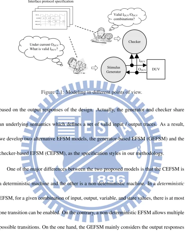
Most interface protocols are written in natural languages or waveform diagrams. Like other automation methodologies, we need to formally specify the interface protocol first. Interpreting an interface specification is like to specify what is valid I/O traces. As shown in Fig 2.1, according to the target simulation components, engineers are used to interpret a specification in either generator’s or checker’s point of view. From a checker’s viewpoint, it observes the behaviors of IDU V and ODU V simultaneously to determine whether the current trace is valid or not. From a generator’s viewpoint, it produces valid input stimuli

Checker DUV Stimulus Generator IDUV ODUV

Interface protocol specification

Valid IDUV/ODUV

combinations?

Under current ODUV

What is valid IDUV?

Figure 2.1: Modeling in different points of view.

based on the output responses of the design. Actually, the generator and checker share an underlying semantics which defines a set of valid input / output traces. As a result, we develop two alternative EFSM models, the generator-based EFSM (GEFSM) and the checker-based EFSM (CEFSM), as the specification styles in our methodology.

One of the major differences between the two proposed models is that the CEFSM is a deterministic machine and the other is a non-deterministic machine. In a deterministic EFSM, for a given combination of input, output, variable, and state values, there is at most one transition can be enabled. On the contrary, a non-deterministic EFSM allows multiple possible transitions. On the one hand, the GEFSM mainly considers the output responses of the DUV and the internal state to define the valid stimuli to the DUV. Since the multiple valid stimuli are usually allowed under certain output responses, the state transitions of the GEFSM are non-deterministic which is more intuitive and flexible to write a generator. On the other hand, the structure of the CEFSM imitates a real checker which considers

Table 2.1: Comparisons among two EFSM models

Model Input Output State transition Independent checker?

GEFSM ODU V IDU V N on − deterministic N o

CEFSM IDU V ∪ ODU V N one Deterministic Y es

all the input and output signals as the state transition conditions. Table 2.1 shows the basic comparison between them. Each of the two models can be translated to a complete simulation kit. However, there is a slight difference between the two translated kits. The CEFSM-based correctness checker can operate correctly with other stimulus generators / testbenches. But the GEFSM-based correctness checking ability can only accompany the GEFSM-based stimulus generator.

2.2 The Flow of Our Methodology

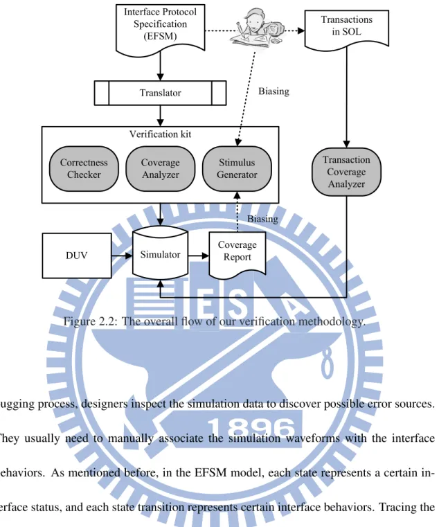
The flow of our methodology is illustrated in Fig. 2.2. The interface protocol specifica-tion is expressed with a modified EFSM model initially. The model can be translated into a stimulus generator, a correctness checker, and a structural coverage analyzer. Mean-while, the interested transactions can be specified using SOL. These transactions are fur-ther translated into a functional coverage analyzer automatically. Then the whole system, including the DUV, stimulus generator, correctness checker, and coverage analyzer, is simulated. According to the outcome from the correctness checker, we can know if the DUV conforms to the interface protocol. The EFSM-based checker can not only detect protocol violations, but also provide useful information for debugging. In traditional

de-Verification kit DUV Biasing Interface Protocol Specification (EFSM) Correctness Checker Coverage Analyzer Stimulus Generator Translator Simulator Transactions in SOL Transaction Coverage Analyzer Coverage Report Biasing

Figure 2.2: The overall flow of our verification methodology.

bugging process, designers inspect the simulation data to discover possible error sources. They usually need to manually associate the simulation waveforms with the interface behaviors. As mentioned before, in the EFSM model, each state represents a certain in-terface status, and each state transition represents certain inin-terface behaviors. Tracing the simulation sequences via the EFSM model can easily link the simulation data and the desired transactions together. This makes the debugging work simpler and more intuitive. From the coverage analyzer, the report can show how many interested transactions have been verified. Moreover, the coverage information can be used to further guide the biasing options of stimulus generator to hit those unverified corner cases.

2.3 Related Works

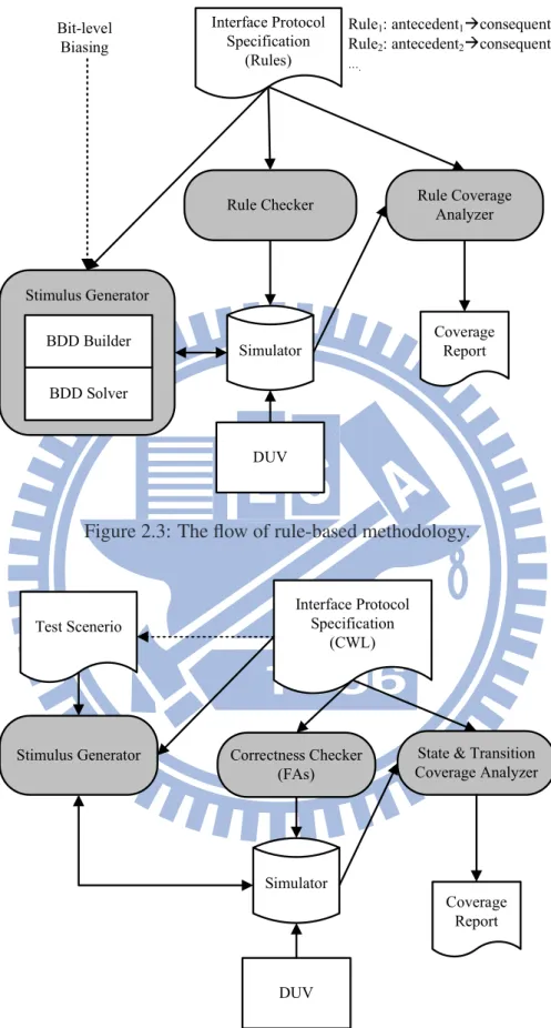
Some research works have been proposed to build a complete simulation environment. In [14], the authors create a list of interface constraints in a proprietary specification style, which is called the “antecedent implies consequent” form. The antecedent and consequent are both Boolean formulae. When an antecedent’s condition is met, the implied conse-quent’s condition must be held simultaneously. These constraints can be directly used as assertions during simulation. This work creates BDDs from the asserted constraints on-the-fly and applies BDD traversals to find a valid stimulus. The coverage metric in this work is defined as the proportion of how many antecedent conditions are triggered during simulation. Fig. 2.3 illustrates this rule-based framework.

Another work proposed by Ara et al. [34] defines valid signal values hierarchically with a regular-expression-based (RE-based) language, CWL (Component Wrapper Lan-guage). These definitions can be converted to corresponding finite automata acting as correctness checkers during simulation. Verification engineers can manually assemble these definitions to develop required stimuli more quickly. How many states and transi-tions of all finite automata are visited is counted as the main coverage measurement in this approach. Fig. 2.4 illustrates the CWL-based framework.

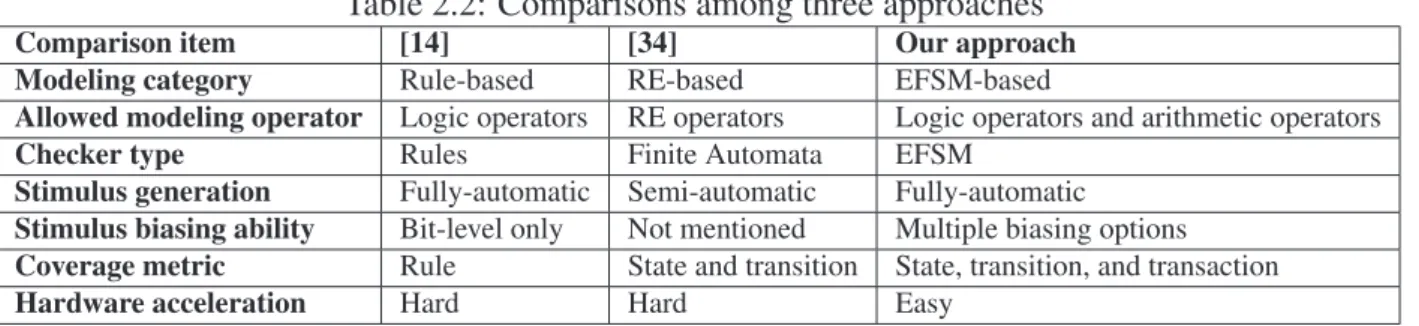
We list the comparisons between the two existing approaches and ours in Table 2.2. Compared to previous approaches, the major contributions of our approach are:

DUV Interface Protocol

Specification (Rules)

Rule Checker Rule Coverage

Analyzer Stimulus Generator Simulator Coverage Report Bit-level Biasing

Rule1: antecedent1 consequent1

Rule2: antecedent2 consequent2 ….

BDD Solver BDD Builder

Figure 2.3: The flow of rule-based methodology.

DUV Interface Protocol Specification (CWL) Correctness Checker (FAs)

State & Transition Coverage Analyzer Stimulus Generator Simulator Coverage Report Test Scenerio

Table 2.2: Comparisons among three approaches

Comparison item [14] [34] Our approach

Modeling category Rule-based RE-based EFSM-based

Allowed modeling operator Logic operators RE operators Logic operators and arithmetic operators

Checker type Rules Finite Automata EFSM

Stimulus generation Fully-automatic Semi-automatic Fully-automatic

Stimulus biasing ability Bit-level only Not mentioned Multiple biasing options

Coverage metric Rule State and transition State, transition, and transaction

Hardware acceleration Hard Hard Easy

• Modify the classical EFSM model to ease the description of interface : The refined EFSM model allows a richer set of operators providing better description power.

• Propose a methodology to obtain a set of simulation components from one specifi-cation automatically and these components are also synthesizable to enable hard-ware acceleration during verification.

• Support various stimulus biasing options to increase the stimulus effectiveness.

• Develop a transaction description language, State-Oriented Language (SOL) [35], to precisely evaluate how many interface functions are actually exercised.

Chapter 3

GEFSM-Based Framework

In the chapter, we introduce the GEFSM-based framework to develop a stimulus generator for interface compliance verification. As well, the diversified biasing strategies includ-ing the transition-level, transaction-level, and bit-level/word-level biasinclud-ing provide users higher controllability over stimulus generation. The GEFSM-based stimulus generator is also capable of checking if the DUV conforms to the interface protocol during simula-tion. Furthermore, unlike SAT- or BDD-based constraint solvers, this generator can be easily implemented in synthesizable Hardware Description Language (HDL). Therefore, it is feasible to dramatically speed up the verification process via a hardware accelerator or emulator.

3.1 The Traditional EFSM Model

Definition 1 For a variable v, its value set is Dv.

Definition 2 For a finite set of variables V ={v1, v2, ..., vn}, its value set DV is the

n-dimensional Cartesian product Dv1 × Dv2 × . . . × Dvn.

The EFSM model is a finite state machine extended with internal variables. It provides a more efficient way to describe the behavior of a sequential circuit and relaxes the state explosion problem suffered by traditional finite state machine models.

Definition 3 An EFSM is a 7-tuple (Q, Σ, ∆, X, q0, X0, F,U,T ), where

Q a set of finite states Σ a set of inputs ∆ a set of outputs

X a set of variables

q0 the initial state, q0 ∈ Q

X0 a set of initial values for variables in X

F a set of enabling functions fisuch that fi: DX → {0,1}

U a set of update transformation functions ui such that ui: DX → DX

T a set of state transition relation such that: T : Q × DX × DΣ → Q × DX ×

sidle s1 REQ ACK !REQ s2 s101 !ACK ACK ACK sidle swait REQ / Count=100 ACK /!REQ / -(!ACK)&(Count!=0) / Count--svio (!ACK)&(Count==0) /-svio !ACK

FSM (103 states) EFSM (3 states)

Figure 3.1: A same protocol in two different FSM representations.

Internal variables used in the EFSM model can significantly reduce the number of required states. For example, as shown in Fig. 3.1, if a protocol specifies that a slave can arbitrarily insert up to 100 wait cycles before responding to a master’s request, the classical FSM requires 103 states to model this behavior while the EFSM only needs 3 states.

3.2 The GEFSM Model

Though the EFSM model has been widely used in many previous research works [36] [37] [38], we slightly modify the definition of the state transition to best fit our own need here. The modified model is called the Generator-based EFSM model which can be seem as a protocol specification from the generator’s point of view.

Definition 4 A GEFSM is a 7-tuple (Q, Σ, ∆, X, q0, X0, T ), where

Q a set of finite states Σ a set of inputs

∆ a set of outputs

X a set of variables

q0 the initial state, q0 ∈ Q

X0 a set of initial values for variables in X

T a set of state transitions, each transition t is a 4-tuple (st, qt, et, ut), where st the current state, st∈ Q

qt the next state, qt∈ Q

et the transition enabling function, returning true(1)/false(0) to enable/disable

the transition, et: DΣ× D∆× DX → {0, 1}

ut the update transformation function, updating the values of the subset

S ⊆ ∆ ∪ X, ut : DΣ× D∆× DX → DS

Definition 5 The GEFSM is a non-deterministic machine. That is, for any state s ∈ Q and its outgoing transition set Ts= {t | t = (st, qt, et, ut) ∈ T and st = s}. It is allowed

that ∃ ti, tj ∈ Ts, ti 6= tj and d ∈ DΣ× D∆× DX, s.t. both eti(d) = 1 and etj(d) = 1.

3.3 An Example Protocol Specification

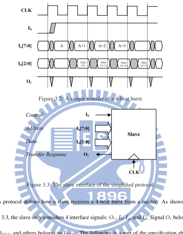
In order to clearly illustrate our methodology, we introduce a protocol simplified from the AMBA AHB [39] as an example. Fig. 3.2 shows the simplest transfer of this protocol.

CLK Ib

Ia[7:0]

I_d[2:0]

Or

A A+1 A+2 A+3

Data (A) Data (A+1) Data (A+2) Data (A+3)

Figure 3.2: A simple transfer of a 4-beat burst.

Slave CLK Ib Ia[7:0] Id[2:0] Or Control Address Data Transfer Response

Figure 3.3: The slave interface of the simplified protocol.

This protocol defines how a slave receives a 4-beat burst from a master. As shown in Fig. 3.3, the slave only considers 4 interface signals: Or, Ib, Ia, and Id. Signal Orbelongs to ODU V and others belogns to IDU V. The following is a part of the specification about the bus master issuing a 4-beat burst to a slave:

(Item 1) A 4-beat burst includes 4 data transfers. A burst can tightly follow another burst.

CLK Ib

Ia[7:0]

I_d[2:0]

Or

A A+1 A+2 A+3

Data (A) Data (A+1) Data (A+2)

Figure 3.4: A burst with a wait state.

current transfer plus one.

(Item 3) The slave asserts the ready signal (Or) when it is ready for the current transfer. The master should send the values of the current data (Id) and the next address.

(Item 4) A slave can insert extra wait cycles by deasserting Or. In this situation, all output signals of the master must hold their previous values. Fig. 3.4 shows a burst with a wait state added for the first transfer.

(Item 5) The master can choose to continue the burst (Ib = 1) or send a busy response (Ib = 0) to temporarily suspend the next transfer. Fig. 3.5 shows a burst with a busy state added for the second transfer.

According to the protocol specification, we build the corresponding GEFSM step by step as shown in Fig. 3.6 and Fig. 3.7. The final GEFSM Fig. 3.7 is shown which has four states (s0, s1, s2, and s3) and 17 transitions (t1 ∼ t17) with an internal variable (x1) for

CLK Ib

Ia[7:0]

I_d[2:0]

Or

A A+1 A+1 A+2

Data (A) Data (A+1) Data (A+2)

Figure 3.5: A burst with a busy state.

burst-length counting.

3.4 Stimulus Generation Flow

We develop a translator that can automatically translate a given GEFSM model into the corresponding stimulus generator. The generated stimulus generator is capable of produc-ing massive random stimuli which are fully compliant with the given interface protocol via the corresponding GEFSM.

For a GEFSM-based stimulus generator, Fig. 3.8 illustrates the 3-phase flow about how to automatically generate the stimulus on-the-fly based on the current DUV’s re-sponse during dynamic simulation:

1. Evaluation: At the current state, evaluate the enabling functions of all its outgoing transitions. The return values of the enabling functions are determined by the

cur-s1

s0

x1==0 /

-- / x1=4

x1!=0 / x1=x1-1

Step 1 (from Item 1)

s1

s0

x1==0 /

-- / x1=4

x1!=0 / x1=x1-1; Ia= Ia+1;

Step 2 (from Item 1~2)

s1

s0

(Or==1) (x1==0) /

-- / x1=4

(Or==1) (x1!=0) / x1=x1-1; Ia= Ia+1;

Step 3 (from Item 1~3)

s1

s0

(Or==1) (x1==0)

/-- / x1=4

(Or==1) (x1!=0) / x1=x1-1; Ia= Ia+1;

Step 4 (from Item 1~4)

s2 Or==0 / Ia=Ia; Id=Id (Or==1) x1==0) / x1=4 (Or==1) x1==0) / -Or==0 / Ia=Ia; Id=Id / / / / -x1==0 / x1=4 x1==0 / x1=4 (Or==1) (x1==0) / x1=4 (Or==1) (x1==0) / x1=4

s

s

s

s

GEFSM

∑: O

∆: I

, I

, I

State: S

, S

, S

, S

Variable: x

Transition definitions:

t=(s

, q

, e

, u

)

t

=(S

, S

, -, {I

==0})

t

=(S

, S

, -, {I

==1; x

=4})

t

=(S

, S

, (O

==1)

x

!=0), {I

=1; I

=I

+1; x

=x

-1})

t

=(S

, S

, (O

==1)

x

==0), {I

=1; x

=4})

t

=(S

, S

, (O

==1)

x

==0), {I

=0})

t

=(S

, S

, O

==0, {I

=I

; I

=I

})

t

=(S

, S

, (O

==1)

x

!=0), {I

=0; I

==I

+1; x

=x

-1})

t

=(S

, S

, O

==0, I

=I

; I

=I

)

t

=(S

, S

, (O

==1)

x

==0), {I

=0})

t

=(S

, S

, (O

==1)

x

==0), {I

=1; x

=4})

t

=(S

, S

, (O

==1) (x

!=0), {I

=1; I

=I

+1; x

=x

-1})

t

=(S

, S

, (O

==1) (x

!=0), {I

=0; I

=I

+1; x

=x

-1})

t

=(S

, S

, O

==1, {I

=0; I

=I

; I

=I

})

t

=(S

, S

, O

==1, {I

=1; I

=I

; I

=I

})

Step 5 (from Item 1~5)

Evaluation Selection

Update

Figure 3.8: Stimulus generation flow.

rent values of the interface signals (Σ, ∆) and internal variables (X). A transition is put into the next transition candidate set (NTCS) only if its enabling function is evaluated true. Some transitions might be evaluated false and excluded in the NTCS. It actually means the current signal values on the interface prevent the stim-ulus generator from producing certain stimuli for the next cycle. In other words, the stimulus generator implicitly solves constraints presented by the given protocol during the stimulus generation process. Meanwhile, in case the NTCS is empty after the evaluation, it means the behavior of DUV must violate the protocol be-cause it makes the stimulus generator find no valid move for the next cycle. That is, the stimulus generator can not only generate the valid stimuli but also serve as a protocol compliance checker at the same time.

2. Selection: From the non-empty NTCS, randomly pick one as the next transition based on the given transition weights. A transition with a higher weight has a higher probability to be selected as the next transition. Hence, some sort of biasing strate-gies can be utilized here to meet volatile requirements of users. Meanwhile, the next transition becomes determinate at this phase no matter what selection strategy

is in use.

3. Update: Assign values to the outputs and variables according to the update trans-formation function of the selected transition. This phase consists of the constrained and unconstrained parts:

(a) Constrained part: Outputs and variables explicitly defined in the update transformation function must be assigned with the constrained values.

(b) Unconstrained part: Outputs not defined in the update transformation func-tion can be randomly assigned with any valid values within their own domains. Again, some kind of biasing strategies can be used here.

Actually, the mission of the Update phase is to generate a complete and valid stim-ulus. After the Update phase, the GEFSM moves to the next state through the selected transition and then the stimulus generation process goes back to the Eval-uation phase for the next cycle.

Now we use the stimulus generator built from the GEFSM in Fig. 3.7 to demonstrate this flow. Assume the current state is s1:

Case 1 (current state = S1, Ia= 20, Ib = 1, Id = 0, Or = 1, Vb = 3)

The enabling functions et3 and et7 are both evaluated true at the Evaluation phase. It

Next, at the Selection phase, one of the candidates would be chosen as the next transition. Assume the transition t7 is selected, the constrained outputs and variables of ut7 need to

be updated as the defined values – assigning Ia, Ib, and X1 to 21, 0, and 2, respectively.

The remaining unconstrained outputs can be assigned to any valid values. For instance, we can set Idto 2. Finally, the current state moves from s1to s3.

Case 2 (current state = S3, Or= 0)

In this case, all enabling functions return false at the Evaluation phase. In other words, no possible transition exists and a protocol violation is detected by the stimulus generator. Meanwhile, it terminates the current simulation and reports the error.

3.5 Stimulus Biasing

Biasing techniques can help verification engineers generate stimuli to hit desirable corner cases more easily. BDD-based approaches can generally support the stimulus biasing. However, due to the BDD’s inherent topology, only bit-level signals can be biased in these approaches. Instead, our stimulus generator is capable of achieving an even higher flexibility, shown later, to bias the generated stimuli. This feature is extremely useful to exercise those uncovered scenarios to get a better simulation quality.

Table 3.1: Biasing information I

Biasing type Weight

Transition-level Wt3 = 20 Wt4 = 40 Wt5 = 40 Wt6 = 100 Wt7 = 80 Word-level Wd=20_b00= 5 Wd=20_b01= 40 Wd=20_b10= 40 Wd=20_b11= 15

3.5.1 Transition-level Biasing / Transaction-level Biasing

Since each transition indicates certain interface behavior, we use the transition-level

bi-asing to guide the state transition. Due to the non-determinism, there may exist multiple

valid transitions after the Evaluation phase. A strategy is needed to pick one from these candidates. One method is to give each transition t an individual weight wt. Then, the probability that a candidate transition ti is selected is defined as:

Pti =

wti

P

tj∈N T CSwtj

, ti ∈NTCS

For example, in Case 1 of the previous example, t3 and t7 are both transition candidates.

If the biasing information is given as Table 3.1, t7 has a higher probability (80%) to be

chosen than t3(20%) does. Furthermore, if preliminary simulation results do not exercise

certain states or transitions, the related transition weights can be increased accordingly. Another similar approach is the transaction-level biasing. We can define a meaningful transaction in terms of a sequence of transitions and then bias all these transitions at the

d[1] d[1]=1 d[1]=0 (Value) d=2'b11 d=2'b10 d=2'b01 d=2'b00 (Biasing) p*q p*(1-q) (1-p)*q (1-p)*(1-q) p (1-p) d[0]=1 d[0]=0 q (1-q)

(a) (b)

Figure 3.9: An example of bit-level biasing.

same time.

3.5.2 Bit-level biasing / Word-level biasing

As mentioned before, bit-level biasing is available while BDD-based approaches are adopted. The basic idea of these approaches is to traverse BDDs to obtain a valid so-lution. Fig. 3.9 is an example to demonstrate the bit-level biasing scheme. In Fig. 3.9(a), there are two BDD nodes representing distinct bit signals, d[0] and d[1]. Each node has two outgoing branches “Then” and “Else” to indicate that the signal is assigned to 1 or 0. General bit-level biasing schemes set a probability value along with each branch to affect the BDD traversal outcomes. For example, p and q are bit-level biasing parameters for “d[1]=1” and “d[0]=1” in Fig. 3.9, respectively.

In typical protocols, many signals are defined in a group of bits, i.e., a word, instead of a single bit only. Therefore, the capability of the word-level biasing becomes critical

and essential. As shown in Fig. 3.9(b), bit-level biasing settings can result in different word-level biasing. However, bit-level biasing has limitations in many situations. For example, in our approach, we allow the weight settings for different word values of d as shown in Table 3.1 to apply direct word-level biasing. This biasing setting simultaneously increases the appearance probabilities of “d=01” and “d=10”. Note that, under bit-level biasing, the positive biasing of “d=01” implies the negative biasing of “d=10”. Obviously, there is no way for bit-level biasing to achieve the distribution of word-level biasing given in Table 3.1.

In our approach, the word-level biasing settings can affect the generated stimuli in two manners. On the one hand, while the biased signal is in the unconstrained part of the Update phase, the signal’s value can be directly produced via a weighted random number generator with the distribution specified by the word-level biasing. On the other hand, if the biased signal appears in the constrained part, i.e., the signal value relates to which transition is selected, the biasing effect could be reflected by changing the transition weights. Assume the word-level biasing list for an n-bit signal s is “Ws=0, Ws=1, ...,

Ws=2n₋₁” and C_s=it is a binary variable indicating if “s = i” is feasible while selecting

t as the next transition, for 0 ≤ i ≤ 2n_{− 1. While the original transition weight of the} transition t is wt, the modified transition weight according to the word-level biasing is:

w0

t= wt∗

P₂n₋₁

i=0 Cs=it ∗ Ws=i P₂n₋₁

Table 3.2 shows an example of this mechanism. When the word-level weights of the signal b are given, the original transition weights, as shown in Table 3.1, can be modified according to the update transformation functions of those transitions. While t3and t7

con-strain the value of Ib to 1 and 0, respectively, the modification ratio, Wt03/Wt3:W

0 t7/Wt7,

is 3:1, which is the same as the word-level biasing setting of Ib (WIb=1:WIb=0). After

this adjustment, the transitions tending to generate signal values with higher word-level weights should appear more frequently.

3.5.3 Feedback for Biasing Refinements

By understanding the design intent and desired scenarios, engineers can manually change those biasing settings to improve simulation quality in later simulation runs. Besides, we could also build a weight tuner which can collect current simulation information and adjust the biasing settings automatically.

In general, a weight tuner should follow certain formulae or strategies to bias the simulation to unverified corners. In other words, the new weight settings should raise the appearance probability of those stimuli which are seldom or even not produced in the previous stimulus set. For example, here is a simple strategy for increasing the transition coverage of GEFSM and balancing every transition’s appearance count as far as possible. Assume current outgoing transitions are {t1, t2, ..., tn} and the corresponding weight set is W={wt1, wt2, ..., wtn}. If ti is selected as the next transition and wti is greater than n,

Table 3.2: Biasing information II

Biasing type Weight

Word-level WIb=0= 1 WIb=1= 3 Modified weight Transition-level W0 t3 = 80 ∗ (3/4) = 60 W0 t4 = 20 ∗ (3/4) = 15 W0 t5 = 40 ∗ (1/4) = 10 W0 t6 = 100 ∗ (4/4) = 100 W0 t7 = 80 ∗ (1/4) = 20

we can apply the following weight tuning formula to every wtj ∈ W:

wtj =          wtj− n, for j=i wtj+ 1, for j6=i

By decreasing the weight of frequently appeared transition and increasing weights of others, this kind of feedback mechanism can dynamically modify biasing settings during simulation. Hence, more varied stimulus sequences can be obtained using an automatic weight tuner.

3.6 Automatic Translation

We implement an translator as shown in Fig. 3.10. The translator first reads in the given GEFSM of the specific interface protocol and the biasing information. It then automat-ically produces a corresponding stimulus generator in target HDL form. The upper part in Fig. 3.10 is a typical simulation-based verification environment. DUVs are usually written in HDL. However, high-level testbenches or stimulus generators are often

devel-I/F HDL Simulator DUV SG HW-based SG DUV I/F Emulator GEFSM Biasing Information Translator SG Synthesizer Synthesizable Only Behavioral or Synthesizable

Figure 3.10: Stimulus generator translation flow.

oped in C/C++, so they need to interact with the HDL simulator via the Programming Language Interface (PLI). Extra simulation overhead is required due to the PLI commu-nication need. Since our stimulus generator is implemented in native HDL, it can thus save simulation time compared to those approaches using PLI.

Fig. 3.11 shows the interface of the stimulus generator. The primary input ports (Σ) and output ports (∆) of generated stimulus generator are defined in GEFSM model. Be-sides, it has an additional output port, “FAIL”, to indicate whether any violation occurs. This translation process can be finished in the following three steps:

(Step 1) First, the compiler translates the enabling functions into assignment state-ments. For example, the enabling function et3 in Fig. 3.7 can be written with

the following Verilog statement:

GEFSM M=( Q, ∑, ∆, X, q0, x0, T )

AVSG

Figure 3.11: The interface of the stimulus generator.

In this statement, et3 is a binary variable representing the evaluation result. The

evaluation results for all outgoing transitions of the current state pass through an NOR gate and then drive the output signal “FAIL” as shown in Fig. 3.11. As explained, it implies if no available transition for the next move, the DUV must have some design error.

(Step 2) Unlike the deterministic machine, the GEFSM has a set of transition can-didates. In our approach, the stimulus generator chooses the next transition according to the given transition weights (transition-level biasing). We use a weighted selection procedure as shown in Fig. 3.12 to realize this mechanism. First, it sums the weights of transitions in NTCS via additions or a lookup-up table. Then, it generates a random number between 0 and the weight sum. Typ-ically, random numbers can be obtained from a software call provided by most HDL simulators. According to this number and weight distribution, a decoder

can determine the selection result.

(Step 3) The major task of the stimulus generator is to generate proper values for out-put signals which are constrained by the selected transition. On one hand, the constraints are defined in the update transformation functions, and the compiler directly translates them into assignment statements. For example, the update transformation function ut3 can be implemented with three statements in

Ver-ilog:

x1 = x1− 1;

Ia = Ia+ 1;

Ib = 1;

On the other hand, the weighted selection procedure is used to assign the un-constrained output signals with weighted random values (bit-level/word-level biasing).

Synthesizable stimulus generator

Practically, simulation jobs are very time-consuming for large complex SOC designs. Hence hardware accelerators or emulators are usually utilized to speed up the verifica-tion process around 100 ∼ 1000 times. The lower part of Fig. 3.10 demonstrates this acceleration environment. In general, SAT- or BDD-based generators are inherently hard

Adder Tree / Look-up Table Wt1 Wt1+Wt2 Wt1+Wt2+Wt3 Wt1+Wt2+Wt3+Wt4 Decoder < < < < Wt1 Wt2 Wt3 Wt4 Selection Result Random Number Generatior

Figure 3.12: Weighted selection procedure.

to be synthesized to hardware, and thus prevent such kind of acceleration. Conversely, the proposed translator is capable of generating the stimulus generator in synthesizable HDL form on one condition – only synthesizable operators are allowed in the transition enabling and update transformation functions of the given GEFSM. In our experiences, the set of synthesizable operators are generally large enough for modeling most of inter-face protocols. Furthermore, random numbers are required to implement the weighted selection schemes requested by the Selection and Update phases. This hardware imple-mentation is similar to the hardware Lottery manager circuit in [40]. To make our stimulus generator fully synthesizable, a hardware-based LFSR (Linear Feedback Shift Register) [41] is used. The combination of these 2 efforts enables the truly hardware-based stimu-lus generator as well as the use of hardware acceleration techniques. Fig. 3.13 shows the block diagram of the proposed GEFSM-based stimulus generator.

Fail Transition

Evaluator

Random Number Generator / LFSR IDUV ODUV Transition Selector Updater Constrained Stimulus Assignment Unit Unconstrained Stimulus Assignment Unit

Round Robin Selector / Weighted Random

Selector NTCS state

Figure 3.13: The block diagram of the proposed GEFSM-based stimulus generator.

3.7 Experimental Results

To demonstrate the effectiveness and efficiency of our approach, we use the WISHBONE [42] and AMBA AHB protocols as the test cases. The experiments are conducted over a set of 3 WISHBONE-compliant and 3 AHB-compliant bus slave designs. The WISH-BONE test cases are obtained from the OPENCORES organization [43], and the others are internal designs. Table 3.3 shows the basic information of each design. All exper-iments are performed on a Sun Blade-2000 workstation with 1GB RAM. Simulation is conducted using a Cadence Verilog-XL simulator.

We first model both the WISHBONE and AHB protocols in GEFSM. The resultant GEFSM of the WISHBONE requires 4 states and 17 transitions while AHB’s requires 6 states and 46 transitions. Then the target stimulus generators are directly generated from

Table 3.3: Basic information of selected DUVs

Design Description Protocol

AC97 Simple AC97 controller WISHBONE

SPI Serial Peripheral Interface WISHBONE

PTC PWM/Timer/Counter WISHBONE

RGB2YCrCb RGB-to-YCrCb Translator AMBA AHB

CON Convolution Calculator AMBA AHB

MAC Multiply-accumulator AMBA AHB

the corresponding GEFSMs through the proposed compiler.

Overall experimental results confirm that generated stimulus generators are fully ca-pable of providing a large amount of valid verification stimuli for all 6 designs. Next, we report certain detailed experimental results to show the power of biasing and the run-time efficiency of our stimulus generation.

3.7.1 Stimulus Biasing

We apply the proposed biasing methods on the experiments over the design CON. We first show the effectiveness of the transaction-level biasing. Suppose each transition ini-tially has equal weight and users want to exercise a five-cycle transaction, “Nonseq → Busy → Seq → Busy → Seq”. However, this transaction never occurs in the initial unbi-ased simulation of 1000 cycles. Then we increase the weights of related transitions (e.g., Nonseq→Busy) by 10 times. Under the new bias setting, the expected transaction appears 19 times in first 1000 cycles. It demonstrates that the transaction-level biasing technique can help achieve higher functional coverage in shorter simulation cycles.

Table 3.4: Results of word-level biasing

HBURST Burst type Weight Count

000 SINGLE 10 13022 (9.95%) 001 INCR 20 25996 (19.86%) 010 WRAP4 40 52377 (40.02%) 011 INCR4 5 6521 (4.98%) 100 WRAP8 15 19645 (15.01%) 101 INCR8 0 0 (0%) 110 WRAP16 0 0 (0%) 111 INCR16 10 13317 (10.18%)

HBURST. HBURST is a three-bit signal indicating the current burst type as shown in the

first and second columns of Table 3.4. For certain verification need, we set the expected probabilities on different HBURST values in terms of the word-level weights. Note that no single bit-level bias setting on HBURST can produce the identical word-level biasing shown in the third column in Table 3.4. After 1 million simulation cycles, the appear-ance count of each burst type is reported in the last column. The results perfectly match the given bias setting. This experiment also implies that we can disable certain types of stimuli by setting the corresponding weights as zeros. This skill is extremely useful when a DUV does not fully implement all features specified in the interface protocol. In short, through the proposed biasing techniques, it becomes much easier to get the desired stimuli.

3.7.2 Performance Analysis

Shorter stimulus generation time should be always preferred during verification. To illus-trate the performance of the stimulus generation, the run-time is compared with those of

Table 3.5: Run-time analysis of different stimulus generators Stimulus generator Design PRSG Ours SG1 SG2 AC97 117.56 s 123.04 s 136.92 s 139.81 s SPI 19.45 s 24.03 s 36.60 s 37.92 s PTC 14.88 s 17.42 s 31.52 s 33.90 s RGB2YCrCb 11.10 s 12.20 s 23.97 s 24.46 s CON 10.43 s 11.37 s 24.01 s 25.09 s MAC 12.80 s 13.82 s 22.11 s 22.55 s Total 186.22 s 201.88 s 275.13 s 283.73 s Ratio 0.92 1.00 1.36 1.41

other stimulus generation methods. We build four simulation environments which contain different stimulus generators. The run-time (for 1 million simulation cycles) for 6 real de-signs in each simulation environment is reported in Table 3.5. In the first environment, we use a pure random stimulus generator (PRSG) to produce stimuli. This is the most trivial way to generate massive random stimuli at virtually no cost. The second environment is to use our stimulus generator instead of the PRSG. From Table 3.5, the difference of run-time required by the PRSG and our stimulus generator is quite small. It shows our stimulus generator can be as efficient as a PRSG. However, the PRSG generally produces invalid stimuli while ours only generates stimuli fully compliant with the protocol. Be-sides, we use CUDD (Colorado University Decision Diagram) [44] package to build two BDD-based implementations, referred to as SG1 and SG2, which are similar to the

stim-ulus generators in [13] and [14], respectively. Since PLI mechanism is required between the HDL simulator and BDD-solving engine for these two environments, the experimen-tal results show that these two environments take averagely 36% and 41% more run-time than our GEFSM-based approach.

3.7.3 Error Detection

While the GEFSM model describes the target interface protocol, the stimulus generator can also detect those design errors which violate the interface protocol. For demonstrat-ing this feature, we do inject protocol-related errors into designs, and the experimental results show that the stimulus generator can indeed capture all these kinds of design er-rors. We also inject protocol-independent errors to correct designs. For example, one such injected error is to change the internal computing function of the design RGB2YCrCb. As expected, this kind of error can not be detected by our stimulus generator since the er-ror effect does not affect the interface behavior. To detect those internal design bugs, users need to build other checkers to investigate the simulation results and the stimulus generator purely serves as a stimulus generator in this case.

3.7.4 Synthesis Results

As mentioned, our stimulus generator can be easily mapped to real hardware through a commercial logic synthesizer. We use Synoposys Design Vision as the synthesizer under UMC 0.18 technology. The synthesizer reports that only 1.8K and 5.7K NAND2-equivalent gates are required to implement the stimulus generators of the WISHBONE and AMBA AHB protocols, respectively. This result clearly shows that the proposed stimulus generator can be easily and cost-effectively integrated into a high-performance emulator-based verification flow.

3.8 Summary

We propose a GEFSM-based approach for interface compliance verification. In this ap-proach, the GEFSM model is used to represent the interface specification from the gen-erator’s view and then automatically translated into a dedicated stimulus generator. This stimulus generator can produce a large amount of valid random stimuli and simultane-ously check the correctness of the interface behavior. In addition, it can be easily im-plemented in synthesizable HDL to enable the hardware acceleration. By supporting transaction-, transition-, and word-level biasing, the stimulus generator provides users better controllability over where a simulation run heads for. The experimental results demonstrate that these biasing methods do successfully generate appropriate stimuli as expected. Moreover, the extremely low overhead in simulation time shows the remark-ably high efficiency of our stimulus generation. Hence, this approach can indeed improve the simulation quality as well as speed up the verification process.

Although the proposed GEFSM can be translated to a stimulus generator which can also check the simulation traces simultaneously, this approach cannot build a pure checker. That is, the protocol checking mechanism is along with the stimulus generation. This may limit the usage model of the GEFSM-based approach while engineers may sometimes re-quire a pure protocol checker to examine the interface behaviors triggered by another stimulus generator or manual stimuli. In the next chapter, we proposed a CEFSM-based methodology which is capable of producing a single stimulus generator, protocol checker,

Chapter 4

CEFSM-Based Framework

In this chapter, a CEFSM-based unified framework is introduced to generate a complete verification kit for interface compliance verification. Compared to the GEFSM-based ap-proach, the correctness checker translated from a CEFSM can operate under other stim-ulus generation schemes. We also introduce a transaction-level coverage metric which is proper to define transactions within an EFSM.