國
立
交
通
大
學
資訊科學與工程研究所
碩
士
論
文
在營運網路中多埠網通設備之即時捕捉與重播機制
On-The-Fly Capture and Replay Mechanisms for Multi-port Network
Devices in Operational Networks
研 究 生:林昱安
指導教授:林盈達 教授
在營運網路中多埠網通設備之即時捕捉與重播機制
On-The-Fly Capture and Replay Mechanisms for Multi-port Network Devices in
Operational Networks
研 究 生:林昱安 Student:Yu-An Lin
指導教授:林盈達 Advisor:Dr. Ying-Dar Lin
國 立 交 通 大 學
資 訊 科 學 與 工 程 研 究 所
碩 士 論 文
A Thesis
Submitted to Institute of Computer Science and Engineering College of Computer Science
National Chiao Tung University in partial Fulfillment of the Requirements
for the Degree of Master in Computer Science June 2013 Hsinchu, Taiwan
中華民國一百零二年六月
在營運網路中多埠網通設備之即時捕捉與重播機制
學生: 林昱安
指導教授: 林盈達
國立交通大學資訊科學與工程研究所
摘要
利用真實環境測試網路設備可以得到複雜的真實測試流量,但缺點是可能造成網路 中斷且錯誤無法重製。而透過重播真實流量測試網路設備可以重製錯誤,但因為流量重 播工具的限制以及不完整的待測物狀態重建導致不佳的錯誤重製率。為了保留複雜的測 試流量及提升錯誤重製率,我們設計一個新機制,它使用 OpenFlow switch 對待測物進 行自動上/下線與多埠流量重播。當待測物在線上時,此機制對待測物進行監控並捕捉錯 誤流量。為了節省空間,我們只捕捉足夠觸發錯誤的封包長度及封包數量。當待測物下 線時,便重播錯誤流量以進行錯誤標示。我們針對不同類型的錯誤使用不同的減量方式 以有效率地進行錯誤標示。實驗結果顯示,錯誤流量的捕捉只需保留封包的部分內容便 可觸發錯誤。針對第二層設備,保留封包前 46 bytes 就足夠觸發錯誤;而我們的第三層 設備只需留下前 154 bytes。封包數量則是依測試環境而異。在錯誤標示方面,我們針對 封包欄位造成的錯誤及超載造成的錯誤設計減量方式,這個減量方式是以二元搜尋法為 基礎。我們提出的減量方式對封包欄位造成的錯誤之縮減比率高達 98.8%、超載造成的 錯誤可達 96%。對於因待測物下線而造成的服務中斷時間,我們發現在監控間距為 1 秒、 容許連續錯誤次數為 2 次時,進行待測物下線能最有效地降低服務中斷時間。 關鍵字:網路設備、故障轉移、OpenFlow switch、多埠重播、減量On-The-Fly Capture and Replay Mechanisms for Multi-port Network
Devices in Operational Networks
Student: Yu-An Lin
Advisor: Dr. Ying-Dar Lin
Department of Computer and Information Science
National Chiao Tung University
Abstract
Testing networking devices in the live environment has complex real traffic, but it may cause network interrupt and cannot reproduce defects. Replaying with real traffic to test networking devices can reproduce defects, but the effectiveness of defect reproduction is not high because of the limitation of replay tools and incomplete reconstruction of DUT (Devices Under Test) states. To keep the high complexity of test traffic and also improve the effectiveness of defect reproduction, we design a new mechanism which can allow DUT to automatically be online/offline and process multi-port replay for multi-port networking devices with an OpenFlow switch. We monitor and capture defect traces when the DUT is online. To save the space, we capture partial payload and limited packet count that are enough to trigger the defects. When we detect the DUT failure, we let the DUT be offline and replay defect trace to identify the defect. For efficient defect identification, we process different reductions for different types of defect. The experimental results show that the partial payload in the packets of captured defect traces can trigger defects. The first 46 bytes is enough for Layer-2 devices and the first 154 bytes is sufficient for our Layer-3 device. The packet count of defect trace depends on the testbed. For defect identification, a reduction based on binary searching algorithm is proposed to deal with defects caused by the payload anomaly and defects caused by the busy condition. The downsizing ratio for defects caused by the payload anomaly is up to 98.8% and the one for defects caused by the busy condition is up to 96%. For the outage time of the failover during the DUT failure, the minimum outage time is obtained when the check interval is 1 second and tolerant consecutive failure time is 2.
誌謝
這篇論文能夠完成,首先要感謝的是指導教授 林盈達教授的教導與指引。在老師 們為學生指導論文的過程中,除了提供學生寶貴的教導與建議,更從老師們身上學習到 做研究所須的認真嚴謹。在論文修訂方面,要特別感謝 賴源正教授和 黃仁竑教授提供 的意見及指正。最後要感謝 林柏青教授在修訂論文上所花的精力與時間,使得本論文 的內容更加圓潤充實。 在這兩年的研究所生涯中,要感謝高速網路實驗室的所有成員,不論是在課業、研 究或生活上所給予的支持與建議。此外,還要感謝交大網路測試中心(NBL)與交大計中 的工作同仁所提供的資源與協助,讓我能順利完成我的研究。 最後感謝我的家人,感謝您們長期對我的關心與照顧,讓我能專注於課業與研究上, 昱安在此衷心的感謝。Contents
List of Figures ... v
List of Tables ... vi
Chapter 1 Introduction ... 1
Chapter 2 Background ... 4
2.1 Networking Device Testing ... 4
2.2 OpenFlow Network ... 6
2.3 Related Works ... 6
Chapter 3 Problem Statement ... 8
3.1 Terminology and Assumptions ... 8
3.2 Problem Description ... 10
Chapter 4 On-The-Fly Capture and Replay Mechanisms (OFCR) ... 11
4.1 Overview of OFCR ... 11
4.2 OFCR Live Mode ... 13
4.3 OFCR Replay Mode ... 14
4.4 Implementation Issues ... 18
Chapter 5 Experiments and Result Analysis ... 20
5.1 Experiment Testbed ... 20
5.2 Experimental Results ... 22
5.3 Case Studies ... 28
Chapter 6 Conclusions and Future Works ... 30
List of Figures
Figure 1: Testing architecture. ... 4
Figure 2: Architecture of OFCR. ... 11
Figure 3: Architecture of RRCA. ... 12
Figure 4: Example of live-to-replay failover. ... 13
Figure 5: OFCR live mode. ... 13
Figure 6: OFCR replay mode. ... 15
Figure 7: Example of replay module. ... 16
Figure 8: Reduction module procedure. ... 16
Figure 9: Packet reduction and payload reduction. ... 18
Figure 10: Experimental environment. ... 21
Figure 11: Capture size of L2 switch in a two-dorm testbed. ... 23
Figure 12: Capture size of L2 switch in a one-dorm testbed. ... 24
Figure 13: Capture size of L3 router in a two-dorm testbed. ... 24
Figure 14: Downsizing ratio of reductions. ... 25
Figure 15: Processing time of reductions. ... 26
Figure 16: The efficiency of reduction thresholds. ... 27
Figure 17: Outage time under different failure criteria. ... 28
List of Tables
Table 1: Comparisons of testing. ... 5
Table 2: Comparisons of capture and replay tools. ... 6
Table 3: Description of notations. ... 9
Chapter 1 Introduction
Networking devices are required to be robust, as they are the cornerstone of the Internet. Networking device testing, which finds out the defects of networking devices and fixes them before product sale, can improve the correctness and robustness of networking devices. By observing the behaviors of DUTs (Devices Under Test) in a testbed, engineers can analyze the defects for debugging. The effectiveness of defect discovery on networking device testing in diverse testbeds can be different with various traffic, testing approaches and replay tools.
Artificial Traffic vs. Real Traffic
The traffic used in networking device testing can be classified as artificial traffic and
real traffic. The former is generated with protocol modeling [1, 2, 3]. Artificial traffic is easy
to produce test cases for specific protocols, but it usually lacks sufficient diversity and complexity. The latter is captured from live environment [4, 5]. Real traffic contains complex network scenarios such as peer-to-peer (P2P), streaming, on-line games, etc. These scenarios are hard to be emulated by modeling, so real traffic is more effective in defect discovery than artificial traffic.
Live Testing vs. Replay Testing
Two main approaches can be used to test networking devices: live testing and replay
testing. The former deploys DUTs in a real-world environment for testing, while the latter
deploys DUTs in a closed testbed and replays captured traffic. Live testing is more effective in defect discovery than replay testing because some defects, such as the defect caused by race condition, only appear in a specific state of a DUT. Those defects may not be triggered in replay testing in a different DUT state. Despite the advantage of live testing, the drawbacks are that the defects are not reproducible, and can cause unexpected network interrupt. Thus live testing provides little information for defect debugging and influences the service quality. Although replay testing produces limited defects, it can replay specific defect-triggering traffic to a DUT many times without influencing the network service quality. Hence, replay testing is more useful for defect debugging than live testing.
Replay tools can be stateless or stateful. The stateless tools like TCPreplay [6] and Tomahawk [7] replay packets based on the timestamps of the packets, but these approaches are not useful for some DUTs which need to keep the state of each network connection. To reproduce the behavior of connections, stateful replay tools modify the content of network trace according to the responses of the DUTs [8-14]. For example, SocketReplay [11] will produce dummy packets to maintain TCP connections.
Depending on the number of ports on a DUT, the replay can be either two-port or
multi-port. The two-port replay sends traffic from one port to the other through the DUT to
reproduce defects. The aforementioned replay tools are all used for two-port DUTs. Nonetheless, we may face a problem in multi-port DUT replay: Some defects are triggered by the interaction of traffic from multiple ports. Replay tools working with two-port DUTs are unable to reproduce the scenario. If a multi-port DUT is used to replay, splitting the traffic for each replay port and synchronizing the replay ports during replay are the challenge.
For improving the efficiency and accuracy of multi-port networking device testing, we focus on defect discovery, replay accuracy and debugging efficiency. How to find defects is an important issue in networking device testing. Because real traffic is better than artificial traffic in defect discovery, we capture real traffic through a DUT in live testing. But when the DUT breaks down, it influences the operational network. In order to reduce the influence of network interrupt, we need a mechanism to allow traffic bypassing the DUT as soon as possible. For the replay accuracy, since most replay tools do not work well for multi-port DUTs, we need a new replay mechanism for multi-port DUTs to reconstruct the defect scenario as one in live environment. For debugging efficiency, the raw captured packet traces are usually huge. We need a method to identify the minimum subset of defect-triggering traffic, so that the storage to save the traffic can be saved and the packet traces of defect-triggering can be reduced.
In this work, we aim to improve the efficiency and accuracy of networking device testing. A mechanism, called OFCR (One-The-Fly Capture and Replay), changes the circuit automatically for defect discovery and reproduction. When a DUT is in a normal state, we perform live testing for the DUT and buffer real traffic simultaneously. While the DUT breaks down, we bypass live traffic and shift the DUT to a replay testbed automatically. When the DUT is in the replay testbed, we use the captured traffic before the breakdown to reproduce and identify the defect. We implement live traffic bypass and replayed traffic split and mix in
an OF switch (OpenFlow[17] switch) instead of using expensive devices: bypass switch and aggregator switch. For defect identification, we find a minimum subset of captured trace by using binary search to keep the least number of packets and the shortest length of payloads.
The remainder of this paper is structured as follows. Chapter 2 presents the background. Chapter 3 describes the assumption and problem statements, and Chapter 4 describes the architecture and implementation issues of OFCR. The experimental results and case study are presented in Chapter 5. Finally, we conclude this work and discuss the future works in Chapter 6.
Chapter 2 Background
This chapter underlines the overview of networking device testing, as well as the architecture of OpenFlow network. Finally, it discusses the related works.
2.1 Networking Device Testing
We categorize networking device testing by testing traffic into four types, including
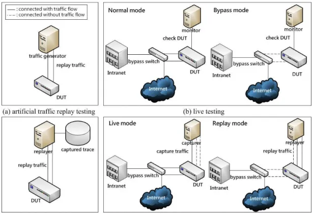
artificial traffic replay testing, live testing, real traffic replay testing and real-time capture and replay testing. Figure 1 presents the architectures of the networking device testing of the four
types.
Figure 1: Testing architecture.
Figure 1 (a) presents the artificial traffic replay testing. We deploy the DUT and the traffic generator in a closed testbed, and the traffic generator will send traffic to the DUT. The traffic is produced by network debugging tools like SmartBits, Codenomicon, etc. Figure 1 (b) presents the live testing. This testing deploys DUT in a live environment. To handle network interrupt when the DUT fails, a monitor is used to check the DUT and a bypass switch is used
to allow traffic bypass the DUT when the DUT failure. Live testing is in the normal mode when the DUT works correctly. In this mode, the traffic passes through the bypass switch as if DUT connects to live network directly. When the monitor detects a failure, it will switch to the bypass mode. In this mode, the ports connected to DUT will close and the traffic will bypass the DUT. In Figure 1 (c) presents the real traffic replay testing, which is in a closed testbed. This testing replays traffic captured from a live environment by replay tools like TCPreplay. Figure 1 (d) presents the real-time capture and replay testing. This testing has two modes: live mode and replay mode. The live mode is similar to the live mode in live testing, but the difference is that the machine not only checks the DUT but also buffers live traffic. When the failure is detected, it will turn to the replay mode. Like live testing, the bypass switch will allow traffic bypass the DUT. At the same time, the replayer can replay the traces buffered earlier to reproduce defects for debugging.
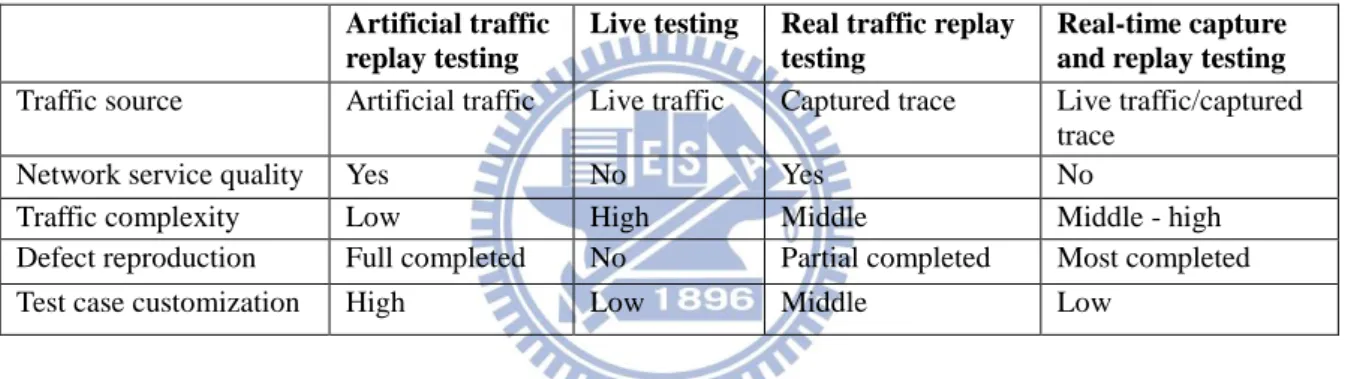
Table 1: Comparisons of testing.
Artificial traffic replay testing
Live testing Real traffic replay testing
Real-time capture and replay testing
Traffic source Artificial traffic Live traffic Captured trace Live traffic/captured trace
Network service quality Yes No Yes No
Traffic complexity Low High Middle Middle - high
Defect reproduction Full completed No Partial completed Most completed
Test case customization High Low Middle Low
We compare the four types of testing in Table 1. In spite of the simplicity of traffic, the advantages of artificial traffic replay testing are the ability of reproducing all defects and good test case customization. The customization of test cases is high because most traffic generators can configure the property of generated traffic. On the contrary, live testing keeps the reality of traffic, but it sacrifices service quality for unexpected network interrupts by DUTs. Moreover, it cannot reproduce the event and has bad test case customization either. Real traffic replay testing is the compromise between the first two types of testing. It uses captured real traffic to improve the complexity and keep the ability of defect reproduction. But the ability of defect reproduction is worse than live testing because of the limitation of replay tools and replay scenarios. It has good service quality as a closed testbed is used, and the customization is better than live testing because we can categorize the collected traces into several groups for testing. Real-time capture and replay testing has better traffic complexity than real traffic replay testing because it deploys the DUT online to encounter some un-reproducible defects, and it has better defect reproduction because more similar replay
scenario than real traffic replay testing. But the tradeoff is the network interrupt when the mode switching. Because the test cases depend on the live traffic, its customization is as low as live testing.
2.2 OpenFlow Network
OpenFlow is a protocol which provides access to the data plane of networking devices. It separates the control plane and the data plane, so that the forwarding path of networking devices can be decided by a remote controller. Administrators can change the network topology from a software controller, significantly enhancing the flexibility of network traffic management.
An OpenFlow network consists of two components: OF switch and OF controller. An OF switch transmits data packets according to a flow table and interacts with the OF controller by a secure channel. When a packet arrives, the OF switch will check its flow table first. If the packet does not match any rule in the flow table, it will be sent to the controller through the secure channel. The OF controller will make a decision for this packet and add a rule into the flow table. When the next packet that belongs to the same flow arrives, the OF switch can handle it by this rule. There are many powerful OF controller implementations like NOX/POX [18], Beacon [19], Floodlight [20], etc. By programming the controller, administrators can control traffic as they want.
2.3 Related Works
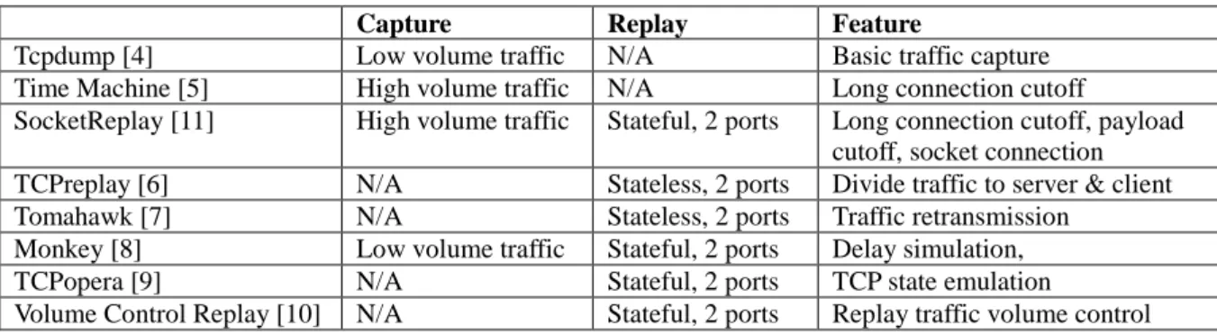
Some popular traffic capture and traffic replay tools are discussed in this subsection and their comparisons are summarized in Table 2.
Table 2: Comparisons of capture and replay tools.
Capture Replay Feature
Tcpdump [4] Low volume traffic N/A Basic traffic capture Time Machine [5] High volume traffic N/A Long connection cutoff
SocketReplay [11] High volume traffic Stateful, 2 ports Long connection cutoff, payload cutoff, socket connection TCPreplay [6] N/A Stateless, 2 ports Divide traffic to server & client Tomahawk [7] N/A Stateless, 2 ports Traffic retransmission
Monkey [8] Low volume traffic Stateful, 2 ports Delay simulation, TCPopera [9] N/A Stateful, 2 ports TCP state emulation
There are several studies related to capture losses and storage space saving. They are all developed from base traffic capture – Tcpdump[4], which is useful with low volume traffic but is inefficient with high-speed traffic because of the frequent system interrupts. To reduce capture losses, many studies use filtering. The study in [5] only records the beginning of all connections to reduce losses and save storage. The study in [11] improves this approach by recording only the beginning of all of the connections and the first part of packets.
Replay tools can be either stateless or stateful. Stateless replay tools send traffic according to the timestamps of packets. TCPreplay [6] can split traces to simulate the behavior between the server and the client through two interfaces. Tomahawk [7] is similar to TCPreplay, but it can retransmit packets when the packets are dropped. Stateful replay tools can keep the states of connections like TCP during replay. SocketReplay [11] maintains the TCP connection state by creating new socket connections. TCPopera [9] emulates the states for each TCP connection. Monkey [8] focuses on TCP replay, and it uses the socket interface to keep the connection state and simulate the delays in connections. The study in [10] focuses on the effectiveness of stateful replay, it can dynamically change the volume of generated traffic during replay. To improve the effectiveness of defect reproduction, we need to build a replay environment which is the most similar to the defect-triggering environment. Despite the above replay tools can be used for stateless and stateful devices, they are insufficient to reconstruct the replay environment for multi-port networking devices. Because these tools cannot split traffic during replay, they cannot reproduce some defects caused by the interaction of multi-port traffic such as the overloads of two different VLANs in a switch.
Chapter 3 Problem Statement
It is obvious that real-time capture and replay testing is effective, but it is not suitable for multi-port devices because of the limited number of ports in the bypass switch and the replay tools. The OF switch is a good choice for traffic handling like bypassing the DUT and splitting during replay. The purpose of this work, namely OFCR, is to combine the real-time capture and replay testing with the OF switch to construct an effective testing for multi-port DUTs. This chapter highlights the terminology and assumptions, and then discusses the problem statement.
3.1 Terminology and Assumptions
In this work, the term traffic is defined as dynamic packet flow in network, and trace is the static file which records the packet flow. A trace that records the traffic causing failures is a defect trace. Not all defects can be reproduced because some defects are due to a non-reproducible scenario like race condition. For a defect trace with reproducible defects, we call it a defect-triggering trace. Here we classify reproducible defects into two types:
overload defect and protocol defect. Overload defect is caused by a busy condition in the
DUT such as hardware overload and table overflow, while protocol defect is triggered by specific content in packets, such as too short or too long payloads and content anomaly.
The procedure in OFCR can be divided into three stages: live mode, live-to-replay
failover and replay mode. Most of the time in OFCR is in the live mode. It records the defect
traces when the DUT fails from a normal state. In order to save the storage, we set thresholds to limit the number of packets and maximum packet lengths when capturing traffic. Live-to-replay failover is a transition between the live mode and replay mode. It changes from live mode to replay mode when the network breaks down due to the DUT failure. It modifies the flow table in the OF switch to keep the network alive and deploy a multi-port replay circuit. Similarly, it can change from the replay mode to live mode when the DUT recovers from the failure. In the replay mode, OFCR replays the defect trace to the multiple ports in the DUT. If the DUT fails again after replay, then the trace is a defect-triggering trace and OFCR will process hybrid defect reduction. Hybrid defect reduction contains overload defect
to operate reduction and the latter assumes the defect is a protocol defect. After these two reductions finish, we can derive the minimum defect-triggering trace.
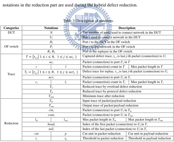
Table 3 is the descriptions of the notations used in this work. There are three types of ports in the OF switch. Di represents the port i to the DUT port Ui, Pi represents the port i to
live network and R1, R2 denote the ports to the two-port replayer. T denotes the defect trace in
traffic capture with total count of packets (connections) c and max packet length l. Inside T, ti,j
represents the last j-th packet (connection) to Ui. When the layer of the DUT is less than four,
the unit is packet, otherwise the unit is connection. uci is the count of packets (connections) to
Ui . The trace used for replaying the defect, Tr,is derived from T. Some packets in T are
incomplete because their original length is larger than l. This will reduce the effectiveness of replay for incomplete packet drop by the network interface, so we process checksum recalculation for packets in T by packet modification tools [14, 15] to derive Tr. When OFCR
operates the hybrid defect reduction, reduced trace To, Tp and Tmin will be generated. The
notations in the reduction part are used during the hybrid defect reduction.
Table 3: Description of notations.
Categories Notations Description
DUT N The number of ports used to connect network in the DUT
Ui Port i used to connect network in the DUT
OF switch
Di Port i to the DUT in the OF switch
Pi Port i to live network in the OF switch
R1, R2 Port to the replayer in the OF switch
Trace
𝑇 = {𝑡𝑖,𝑗| 1 ≤ 𝑖 ≤ 𝑁, 1 ≤ 𝑗 ≤ 𝑢𝑐𝑖 } Captured defect trace, ti, j is last j-th packet (connection) to Ui
uci Packet (connection) to port Ui in T
c l Packet (connection) count in T Max packet length in T 𝑇𝑟= {𝑟𝑖,𝑗| 1 ≤ 𝑖 ≤ 𝑁, 1 ≤ 𝑗 ≤ 𝑢𝑐𝑟𝑖 } Defect trace for replay, ri,,j is last j-th packet (connection) to Ui
ucri Packet (connection) to port Ui in Tr
cr lr Packet (connection) count in Tr Max packet length in Tr
To Reduced trace by overload defect reduction
Tp Reduced trace by protocol defect reduction
Tmin Minimum trace after reduction
Reduction
Tin Input trace of packet/payload reduction
Tout Output trace of packet/payload reduction
cini Packet (connection) to port Ui in Tin
couti Packet (connection) to port Ui in Tout
lin lout Max packet length in Tin Max packet length in Tout
headi Index of the first packet (connection) to Ui in Tr
taili Index of the last packet (connection) to Ui in Tr
cut p Cut unit in packet reduction Cut unit in payload reduction
3.2 Problem Description
We will face some problems for debugging when dealing with a trace captured during a period of time before the DUT failure. First, the packet count c and the max packet length l of trace T may be insufficient to trigger the defects. Second, defects may not be triggered because the two-port replayer cannot forward traffic to multiple ports Ui like the original
defect-triggering scenario. Finally, even though the captured defect trace Tr is small, it is not
easy to identify the defect-triggering packets in Tr.
The detailed problem description is given as follows. Given a DUT with N ports connecting to network by an OF switch and a trace T captured when the DUT fails. The objectives of our work are (1) finding out minimum c and l in T that can triggers defects, (2) replaying packet ri,j in Tr to multiple ports Ui on the DUT, and (3) deriving the minimum
Chapter 4 On-The-Fly Capture and Replay Mechanisms (OFCR)
In this chapter, we state the overview of OFCR and the details of each module in OFCR. Furthermore, we discuss the implementation issues of OFCR.
4.1 Overview of OFCR
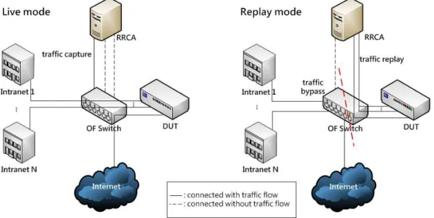
As illustrated in Figure 2, the architectures of OFCR are composed of two modes: the live mode for the DUT normal state and the replay mode for the DUT failure state. In the live mode, as illustrated in the left part of Figure 2, the OF switch not only forwards bidirectional traffic between live network (Intranets and Internet) and the DUT but also mirrors traffic to the RRCA (Remote Replay and Control Agent). The RRCA checks the DUT states and buffers the mirrored traces. In the right part of Figure 2 is the replay mode. In this mode, OF switch separates the network into two parts. The left part is live network, and the right part is the multi-port replay network. The RRCA extracts the defect traces from the buffered traces, and then replays them to the DUT. To process multi-port replay on different layer DUTs, OFCR uses existing two-port replay tools and splits replayed traffic on the OF switch. If the defects can be triggered by multi-port replay, OFCR will process defect identification to find the minimum defect-triggering trace. Defect identification uses hybrid defect reduction involving overload defect reduction and protocol defect reduction. The hybrid defect reduction processes the above two reductions sequentially to identify defects. Finally, we derive the minimum defect-triggering traces from the results of hybrid defect reduction.
The mechanism switching between the two modes is called live-to-replay failover. The major objective of live-to-replay failover is to recover from network interrupt caused by the DUT failure in the live mode as soon as possible. The details of live-to-replay failover will be discussed later.
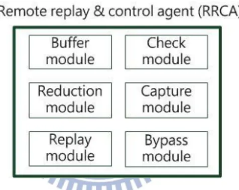
All modules worked in RRCA are shown in Figure 3. In the live mode, two modules are active, the buffer module and the check module. The buffer module is used to buffer the mirrored traces, and the check module checks the DUT state. When the OFCR is in the replay mode, there are four modules operating including the check module, the capture module, the
replay module and the reduction module. The check module is the only module used in both
modes. The capture module is used to store the defect traces. The replay module processes multi-port replay and the reduction module identifies the defect in the defect trace. Finally, the
bypass module doesn’t belong to the live mode or replay mode, it processes live-to-replay
failover.
Figure 3: Architecture of RRCA.
Bypass Module
Live-to-replay failover is operated by the bypass module in OFCR. The bypass module changes the flow table in the OF switch based on the mode of OFCR. The OF switch forwards incoming packets from port Pi to Di, so that packets pass through the DUT for testing in the
live mode, where Pi is port i to live network and Di is port i to the DUT in OF switch. When
OFCR switches to the replay mode because of the DUT failures, the bypass module needs to cut off the connections between Pi and Di and builds a backup circuit. Therefore, a
pre-defined configuration file is essential for the bypass module to modify rules in the flow table to let packets pass through ports Pi.
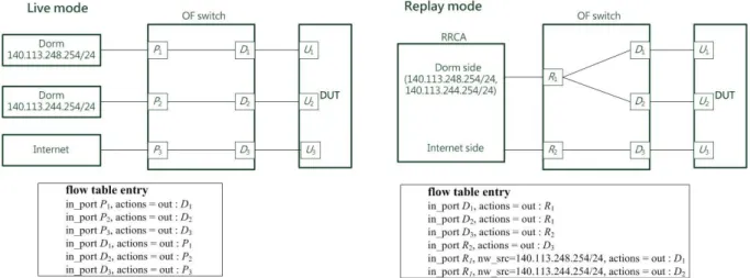
Figure 4 is an example of live-to-replay failover. The DUT connects to two dorms and Internet through an OF switch. The entries in the flow table are one-to-one mapping between
entries about Di will be introduced in the replay module. The bypass module will build the
rules of relationship between Pi by a pre-defined configuration file.
Figure 4: Example of live-to-replay failover.
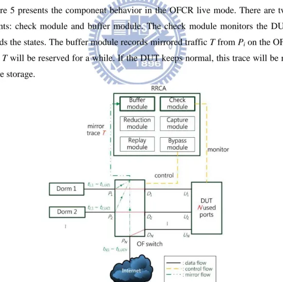
4.2 OFCR Live Mode
Figure 5 presents the component behavior in the OFCR live mode. There are two main components: check module and buffer module. The check module monitors the DUT states and records the states. The buffer module records mirrored traffic T from Pi on the OF switch.
The trace T will be reserved for a while. If the DUT keeps normal, this trace will be removed to save the storage.
Check Module
The check module is responsible to check the status of DUT by probing the DUT to be explained in subsection 4.4. To collect information for the defects, the check module accesses and records the DUT states in several ways like SNMP and console port. The states can be categorized into common states and specific states. The former states are CPU usage, memory usage, bandwidth usage and error logs. The latter states depend on the layer of the DUT, and can be the MAC table and the ARP table in switches, and the ARP table and the routing table in routers.
Buffer Module
The buffer module captures mirrored traffic T continually with c packets (connections) and the maximum packet length l bytes. The capture size has a tradeoff between memory storage and defect effectiveness. The packet count c influences the defect reproduction and memory space, and the maximum packet length l influences the defect reproduction and packet losses. The capture size depends on the traffic volume of the testbed and the layer of DUT. Because common networking devices only have 1~4 ports for traffic mirror, it is easy to encounter the bandwidth overload problem on mirror port. The buffer module can apply many-to-many mirroring by setting the flow table rules in the OF switch. This approach can resolve the bandwidth overload problem to generate less packet losses and also allocate diverse mirror groups for the intranet and internet to reduce the overhead of replay pre-processing.
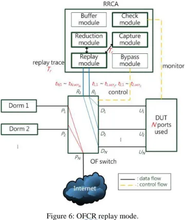
4.3 OFCR Replay Mode
Figure 6 is the components in the OFCR replay mode. The four major components in this mode: check module, capture module, replay module and reduction module. The check module does the same job as it is in the live mode, it is used to determine the effectiveness of the defect trace replay. The capture module extracts the defect trace Tr from buffer module in
the live mode. The replay module forwards packet ri,j to different ports Di in order to transmit
to the proper ports Ui in the DUT, where ri,j is last j-th packet (connection) to the DUT port Ui
in Tr. The reduction module downsizes the defect-triggering trace Tr to derive the minimum
trace Tmin. According to the type of the defect, the reduction module uses different reduce
Figure 6: OFCR replay mode.
Capture Module
The capture module extracts the defect trace from the buffered trace T. The defect trace
Tr has the same capture size cr = c, lr = l. The packet (connection) count to DUT port Ui ucri
may not be equal to uci because the DUT ports for replay can be different from the live mode
when processing multi-port replay. The maximum packet length l may produce incomplete packets during capturing, so the capture module needs to recalculate the checksum of each packet in Tr to derive packet ri,j.
Replay Module
The replay module replays Tr to trigger defects. To reconstruct similar scenario as the
DUT in the live mode, we replay each packet in Tr to the original DUT port as the live mode,
ucri = cri for i = 1…N. It splits Tr into the Intranet side and Internet side, and then replays Tr
from ports R1 and R2 depending on which side the packet (connection) belongs. To forward
packets ri,j to the corresponding port Di, the OF switch splits incoming packets by source IP
addresses. The relations between source IP addresses and ports also need to be defined in a pre-defined configuration file. Figure 7 is the example of the replay module. There are two dorms in the live mode, so the OF switch splits the packets from R1 to D1 and D2 by their
Figure 7: Example of replay module.
Reduction Module
The reduction module identifies defect-triggering traces by hybrid defect reduction. It assumes the defect is overload defect and protocol defect, and then applies the overload defect reduction and the protocol defect reduction respectively. As illustrated in the left part of Figure 8, the hybrid defect reduction processes two reductions sequentially and derives two reduced trace To and Tp. The reduced traces To and Tp are generated by the overload defect
reduction and protocol defect reduction. We can determine Tmin by comparing the traces To, Tp
and the original defect trace Tr.
There are two situations to derive the minimum trace Tmin. (1) If To = Tr and Tp = Tr, it
means that Tr is not a defect-triggering trace or Tr is the minimum defect-triggering trace with
no redundant packets. So we set Tmin as Tr. (2) Otherwise, we keep both reduced traces Tmin =
To ∪ Tp. Because two reduced trace To and Tp may be different in packet (connection) count
and max packet length, we preserve both traces to maintain more information for debugging.
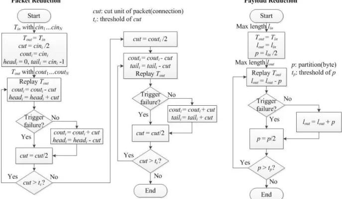
In the right part of Figure 8 is the procedure of the overload defect reduction and the protocol defect reduction. Because the overload defects are usually caused by too many packets and the number of defect-triggering packets is unclear, when we process the reduction of packets, the results will be quite different each time. Therefore, to minimize the size of reduced trace, the overload defect reduction removes redundant payloads first, and then concentrates on reducing packet count. In contract, protocol defects are caused by a single or a few packets. To save processing time of replay in reduction, the protocol defect reduction downsizes the number of packets first and then finds critical parts of payloads.
Figure 9 is the flowchart of packet reduction and payload reduction with binary search. The input trace of the reduction is Tin, the trace Tin is the subset of Tr and has two properties
cini and lin. cini presents packet (connection) count through DUT port Ui and lin means the max
packet length. The output trace of the reduction is Tout. Similarly, Tout has couti and lout. These
two reductions have cut units cut or p respectively, and they have thresholds tc and tp
respectively to stop the reduction. When the cut unit meets the threshold, the reduction stops and generates Tout. Packet reduction removes redundant packets before/after the
defect-triggering part. We use headi and taili to present the indexes of the first and the last
packet (connection) to port i in the reduced trace Tin, the packet with index between headi and
taili will keep in Tout. The left part of packet reduction in the figure deals with the packet
reduction before the defect-triggering part, and the right part handles the reduction after the defect-triggering part. When the layer of devices is larger than 3, the cut unit cut changes to connection. The packet reduction will cut entire connection during reduction because incomplete connection cannot reproduce the connection state. The procedure of payload reduction is simpler than the one of packet reduction, because it only reduces the max packet length of the reduced trace Tin.
Figure 9: Packet reduction and payload reduction.
4.4 Implementation Issues
In this subsection, we discuss the implementation issues on traffic capture and failure detection. The captured traffic may lose packets in the mirror module in the networking devices and capture interfaces in RRCA. Common networking devices only have 1~4 ports supported for traffic mirroring. The traffic volume of mirrored ports is easy to exceed the bandwidth of mirror port. To reduce packet losses in that situation, we use the OF switch to deploy several mirror ports. For packet losses on network interfaces in the RRCA, we add memory and use an improved traffic capture tool, Gulp [21]. Gulp uses ring-buffer and allocates the packet reader and writer in different CPUs to reduce packet losses. Furthermore, the buffer module records traces by add a number which is in a loop in the end of trace file name, it is used to prevent the situation that the defect-triggering packets are recorded in the end of the first trace and the beginning of the second trace, but because we buffer a single trace at a time, we only get the second trace finally.
Failure detection is important because it is the key of mode switching in RRCA. The tool used in the check module is called CheckDev which is developed by NBL [22]. It sends ARP, ICMP and HTTP requests to the DUT so as to probe the DUT status. Moreover, it retrieves the detailed DUT states by the SNMP and console ports. Because of the diverse commands in console port for different DUTs, we write specific scripts by Expect [23] to dump the state
information from the DUT. Another implementation issue in the failure detection is the failure criteria. If the failure criteria are too loose, we will lose some defect traces; otherwise, we will get more defect traces and process more live-to-replay failover. There may be some normal traces in the defect traces. It is hard to distinguish normal traces and un-reproducible defect traces from defect traces because they both don’t trigger any failure when replay. The check module implements the failure criteria by three parameters: check interval, check timeout and tolerant consecutive failure time. We use these three parameters to control live-to-replay failover and keep the effectiveness of defect traces.
Chapter 5 Experiments and Result Analysis
The experiment environment and results will be discussed in this section. In 5.1, we introduce the details about the used testbed in this work. Then we discuss the experimental results from the perspectives of the venders and users. Finally, we analyze the cases about the defect traces.
5.1 Experiment Testbed
The defects triggering in live environment are un-custom. It is hard to collect the defects of specific protocol on specific DUT efficiently, so we use debugging tools to generate specific protocol traffic for DUT used in the experiments. If the generated traffic triggers a defect on the DUT and it can trigger defect by replaying, we capture it as a defect-triggering trace for the experiments. For the reproduction of experiments, we also capture a period of dorm traffic as a normal trace used in the experiments. The testbed is presented in Figure 10. The testbed is composed of two steps. The first step is collecting normal/defect-triggering traffic which is in both sides of the figure. The left side is normal traffic collection. We mirror the dorm traffic in NCTU BetaSite as the normal traffic. The right side is defect-triggering traffic collection. Here we use the debugging tools TestCenter and Codenomicon to trigger DUT defects and capture the defect-triggering traffic. The DUTs we used are ZyXEL GS-2750 and SuperMicro SSE-G24-TG4. ZyXEL GS-2750 is an L2 (Layer-2) switch, SuperMicro SSE-G24-TG4 is an L3 (Layer-3) router and the RRCA is a PC which is equipped with Intel i3-2130 processor, 8GB memory and 9 network interfaces. After finishing normal and defect-triggering traffic collections, we conduct the experiments as the middle part of Figure 10. Because the OF switch TL-WR1043ND is a SOHO AP, it is not capable of handling captured dorm traffic. We use small traffic to process multi-port replay and live-to-replay failover with the OF switch. We process multi-port replay by sending traffic from RRCA to OF switch, then the OF switch passes traffic to the DUT. The connectivity tester is used to measure the effectiveness of live-to-replay failover. We process live-to-replay failover experiments by replaying defect-triggering traces from RRCA to the DUT directly and at the same time probing the connectivity tester though the OF switch. The OF switch transmits the probe messages to the connectivity tester directly or through the DUT according to the DUT state. We use the RRCA and the DUT without the OF switch for the experiments about the traffic capture and traffic reduction because the traffic can overload the OF switch.
Figure 10: Experimental environment.
The details of the normal traces and defect-triggering traces are shown in Table 4. The normal traces are collected from the dorm 9 and 12 in NCTU dorm network. To generate different scale testbeds, we capture the normal traces in one dorm (dorm 9) and two dorms (dorm 9, 12). The protocol defect traces with IP payload anomalies on ZyXEL switch and the OSPF payload anomalies on SuperMicro router are produced by Codenomicon. IP payload anomalies are packets with anomalous fields in the IP header, and OSPF payload anomalies are packets with anomalous fields in the OSPF packet. The overload defect traces on ZyXEL switch are generated by TestCenter, and they have two types: dense ARP requests and dense ICMP requests. Dense ARP requests are used to overflow the MAC table, and dense ICMP requests are used to overflow the ARP table. These two traces can overflow the MAC table and the ARP table in ZyXEL switch.
Table 4: Test traces.
Type Trace count Average size Packet count
Two-dorm traffic Normal 1 918.5MB 818,970
One-dorm traffic Normal 1 446.3MB 368,238
IP payload anomaly Protocol 10 144.7MB 873
Dense ARP requests Overload 1 72.1MB 540,012
Dense ICMP requests Overload 1 864KB 6,331
OSPF payload anomaly Protocol 3 20.3KB 243
To simulate defect-triggering traffic in the live network, we mix a normal trace and a defect-triggering trace. The procedure of traffic mix is replaying a normal trace and a defect-triggering trace to the DUT simultaneously, and capturing them as a defect trace from
the DUT. For L2 devices, we have 12 mixed defect traces for one-dorm environment and 12 for two-dorm environment. For one-dorm/two-dorm environment, these mixed defect traces combine a normal traffic with 10 IP payload anomaly traces, a dense ARP requests trace and a dense ICMP requests trace, so there are 10 protocol defect-triggering traces and 2 overload defect-triggering traces in these 12 mixed defect traces. For L3 devices, we only have 3 OSPF payload anomaly traces. After traffic mix of a two-dorm normal trace and an OSPF anomaly trace, we derive 3 protocol defect-triggering traces for L3 devices.
5.2 Experimental Results
We view the experimental results from the perspectives of the vender side and user side in this subsection. For venders, they care about the effective capture size in the OFCR live mode, the diversity of reduction for different types of defects and the efficiency of reduction thresholds in the OFCR replay mode. For users, the only thing they are concerned about is the outage time during the OFCR live-to-replay failover, so we show the relationship between the failure criteria and the outage time.
Capture Size
The capture size is the first we need to decide when starting OFCR. The parameters c and l influence the effectiveness and size of captured defect traces. We try to find the optimal capture size c and l to balance the above two things for different layers DUTs. The results of L2 switch ZyXEL GS-2750 in the one-dorm and two-dorm environments are presented in Figure 11 and 12, and those of L3 router SuperMicro SSE-G24-TG4 is shown in Figure 13.
Figure 11 presents the effectiveness of defect reproduction for different packet count c and max packet length l in two-dorm testbed. The results show that the first 46 bytes of payload (only ARP/ICMP headers) are enough to trigger all defects. Moreover, capturing 10,000 packets in a trace is sufficient to keep the all protocol defect-triggering packets and 50,000 packets in a trace can keep all defect-triggering packets in 12 mixed defect traces. This is because the overload defect traces need many packets to break down the DUT, packet count
c = 50,000 is enough to capture all defect-triggering packets. When l is less than 46 bytes, we
can find out that it can reproduce only one overload defect trace with c ≥ 50,000. This is because this overload defect is triggered by too many broadcast packets. Even though these captured broadcast packets only include their IP headers, they still can paralyze the DUT.
Figure 11: Capture size of L2 switch in a two-dorm testbed.
We also test the L3 SuperMicro router by these 12 mix defect traces in two-dorm testbed. And we find out that 10 protocol defect traces are not effective because they are defects specific to the ZyXEL switch, but two overload defect traces still can trigger the defects when
l is 46 bytes and c is 50000. So we capture traffic with max packet length l = 46 bytes is
enough to keep the defects for L2 devices.
Figure 12 shows that the results of L2 switch in one-dorm environment. The difference between Figure 12 and Figure 11 is the traffic scale of the environment, and the other factors in these experiments are the same. Because the traffic volume in the one-dorm environment is much smaller than the two-dorm environment, we can reproduce all two overload defect traces with c = 10,000 rather than 50,000 in the two-dorm environment and the reproduction effectiveness of protocol defect trace improves slightly in c = 3,000 and 5,000. To reproduce all protocol defect traces, the capture size of packet count c is 10,000 and the max packet length l is 46 bytes. And when the capture packet count c = 10,000 with max packet length l = 46 bytes can also reproduce all overload defect traces. Therefore, capturing 10,000 packets in a trace and max packet length 46 bytes is enough to reproduce all 12 defect-triggering traces in one-dorm environment. 0 2 4 6 8 10 1000 3000 5000 10000 50000 100000 packet count c Protocol Defect 38 (IP header)
46 (ARP, ICMP header) 78 (with IP option) 154 (ICMP payload) 1522 (Max frame) reproduced trace count
max packet length l
0 1 2 1000 3000 5000 10000 50000 100000 packet count c Overload Defect 38 (IP header)
46 (ARP, ICMP header) 78 (with IP option) 154 (ICMP payload) 1522 (Max frame) reproduced trace count
Figure 12: Capture size of L2 switch in a one-dorm testbed.
Figure 13 is the results of L3 router in the two-dorm environment. There are only three protocol defect traces in this experiment. We need to capture the first 154 bytes to trigger the protocol defects. These protocol defects are triggered by LS (Link State) Update packets in the OSPF, and the OSPF component of the DUT is unable to handle the inconsistency of fields in OSPF packets after it processes LSAs (Link State Advertisement) information after LSA header in the LS Update packet. Because these protocol defects need OSPF payload to trigger defects, the max packet length l depends on max LSA of the router. In our experiment, the SuperMicro router needs first 154 bytes to trigger defects.
Figure 13: Capture size of L3 router in a two-dorm testbed. 0 2 4 6 8 10 1000 3000 5000 10000 50000 100000 packet count c Protocol Defect 38 (IP header)
46 (ARP, ICMP header) 78 (with IP option) 154 (ICMP payload) 1522 (Max frame) reproduced trace count
max packet length l
0 1 2 1000 3000 5000 10000 50000 100000 packet count c Overload Defect 38 (IP header)
46 (ARP, ICMP header) 78 (with IP option) 154 (ICMP payload) 1522 (Max frame) reproduced trace count
max packet length l
0 1 2 3 1000 3000 5000 10000 50000 100000 packet count c Protocol Defect 34 (IP header) 42 (ICMP header) 58 (OSPF header) 78 (OSPF+LSA header) 154 (ICMP payload) 65535 (max IP packet) reproduced trace count
Diversity of Reductions
Because of different properties of the protocol and overload defects, a single reduction will not be suitable for both types of defects. To evaluate the effectiveness of the different reductions, we compare them by the processing time and the downsizing ratio. The processing time is the time from receiving the trace to finishing, and the downsizing ratio represents the relationship between the size of the trace after reduction and that of the original defect trace. The formula is expressed as 𝑑𝑜𝑤𝑛𝑠𝑖𝑧𝑖𝑛𝑔 𝑟𝑎𝑡𝑖𝑜 = 1 −𝑜𝑟𝑖𝑔𝑖𝑛𝑎𝑙 𝑑𝑒𝑓𝑒𝑐𝑡 𝑡𝑟𝑎𝑐𝑒 𝑠𝑖𝑧𝑒𝑟𝑒𝑑𝑢𝑐𝑒𝑑 𝑡𝑟𝑎𝑐𝑒 𝑠𝑖𝑧𝑒 .
We compare five reductions in the OFCR with the protocol defects and overload defects in Figure 14 and 15. The original defect traces have 50,000 packets and the max packet length is 1,522 bytes. The reduction thresholds tc and tp are 1,000 and 10 bytes, respectively.
Figure 14: Downsizing ratio of reductions.
In Figure 14, we can find that the packet reduction and payload reduction are not good on trace downsizing. The protocol defect reduction and overload defect reductions have the same downsizing ratio (98.8%) on the protocol defects, but the overload defect reduction has better downsizing ratio on the overload defects up to 96%. The hybrid defect reduction chooses the best result from the protocol defect reduction and overload defect reduction, so it certainly has the best downsizing ratio.
92.0 87.3 98.8 98.8 98.8 82.6 79.1 91.6 96.0 96.0 75% 80% 85% 90% 95% 100% Packet Reduction Payload Reduction Protocol Defect Reduction Overload Defect Reduction Hybrid Defect Reduction Protocol Defect Overload Defect
Figure 15: Processing time of reductions.
Figure 15 shows the results of processing time of different reductions. The processing time of the protocol defects is longer than that of the overload defects in each reduction. The reason is that there are a few defect-triggering packets in the protocol defect traces, so protocol defect traces need to take more turns to replay the reduced trace during the reduction. Because the packet count influences the replay time significantly, the packet reduction and protocol defect reduction which reduces packet counts first will take shorter processing time than other reductions. However, considering the downsizing ratio, protocol defect reduction is more efficient than packet reduction because it takes additional 200 seconds to reduce more 6% of the size (up to 98% for protocol defect). But the downsizing ratio of the protocol defect reduction is not sufficient for overload defect (91%), the overload defect reduction spends more 230 seconds to remove additional 4% of the size (up to 96%). The processing time of the hybrid defect reduction is the longest because it is the sum of protocol defect reduction and overload defect reduction.
Efficiency of Reduction Thresholds
The efficiency of the reduction is controlled by tc and tp, which are the thresholds of the
cut unit for packet count and the max packet length, respectively. The results of choosing diverse thresholds in the hybrid defect reduction are presented in Figure 16. The defect traces are also with 50,000 packets and max packet length 1522 bytes. Large thresholds tc and tp will
save the processing time but lower the downsizing ratio. However, when the thresholds tc and
tp are too small, the processing time increases significantly but the downsizing ratio rises
0 200 400 600 800 1000 1200 1400 Packet Reduction Payload Reduction Protocol Defect Reduction Overload Defect Reduction Hybrid Defect Reduction Protocol Defect Overload Defect
limitedly. Given the thresholds tc is 5,000, 1,000 and 500, tp is 50, 10 and 5, we can derive the
best downsizing ratio 98.8% when tc ≤ 1,000 (2% of packet count) and tp ≤ 10.
Considering the processing time, the reduction is the most efficient when tc = 1,000 and tp =
10.
Figure 16: The efficiency of reduction thresholds.
Outage Time vs. Failure Criteria
The defects affect different parts of the DUT. Some defects make the DUT fail slightly, and the DUT can recover from the failure by itself in a short period of time. Some defects break down the DUT, and the DUT cannot be recovered until the administrators reboot it. The outage time is the time when the OFCR spends for switching from live to replay mode during the DUT failure and from replay to live mode when DUT recovers. The connections of users will be disconnected in this period. To reduce the outage time, we detect a failure with different check intervals, tolerant consecutive failure times. The tolerant consecutive failure time is the threshold of the DUT consecutive failure time in a specific check interval and response times, the live-to-replay failover will execute when the DUT consecutive failure time exceeds it. The response timeout is the waiting time for the reply of the probing request. Figure 17 presents the results of different check intervals and tolerant consecutive failure times with 1 second response timeout. Two situations occur in the experiment, a defect triggers in the experiment and no defect triggers in the experiment. The leftmost bar presents the outage time without failover (19 seconds), which is the real failure time of the DUT. We
0 200 400 600 800 1000 1200 1400 97.4% 97.6% 97.8% 98.0% 98.2% 98.4% 98.6% 98.8% 99.0% (500, 5) (500, 10) (500, 50) (1000, 5) (1000, 10)(1000, 50)(5000, 5) (5000, 10)(5000, 50) (tc, tp)
Downsizing Ratio Processing Time
can find out that most failure criteria can reduce the outage time except (7, 3). With the same tolerant consecutive failure time, the smaller check interval is, the less outage time is. Small tolerant consecutive failure time can also reduce outage time, but it is better to larger than one. If the tolerant consecutive failure time is one, we may presume a DUT failure because of the incomplete reply packets or packet losses, and then process meaningless live-to-replay failover.
Figure 17: Outage time under different failure criteria.
5.3 Case Studies
In this subsection, we interpret the protocol defect traces in the test traces. When we use Codenomicon to test ZyXEL switch with IP anomaly traces, the ICMP module of the switch crashes but the switch itself does not detect it. Under no error logs, we try to analyze the packets in the IP anomaly defect trace, and find out that the anomaly is on the flags and fragment offset. Figure 18 is the details about the IP anomalies.
Figure 18 (a) is the anomaly in the flags field of the IP header. The first bit in the flags field is a reserved bit and it should be 0, but here it is 1. Figure 18 (b) is the anomaly which combines the flags and fragment offset anomalies in the IP header. The more bit in the flags field is set to 1 which means there is another fragment, but the value of fragment offset is the maximum value. It is impossible to have another fragment after this packet. This anomaly is hard to be detected because if we check these two fields separately, both of them are correct in that field. However, they become an anomaly when they appear together.
0 5 10 15 20 25 no failover (1,2) (2,1) (1,3) (3,1) (3,2) (3,3) (5,2) (5,3) (7,2) (7,3) (check interval, # tolerant consecutive failure)
Defect Trigger No Defect Trigger outage time (sec)
Figure 18: The example of IP anomaly.
Although the logs in the DUT have no error messages, we still can analyze the defects by accessing other DUT states. We find out that there is no overflow in any tables, and the CPU and memory are not at the busy states. Combining with the information and the behavior of the DUT failure, we can conjecture that a single anomalous packet may generate an exception but it does not break down the relevant component in the DUT. However, consecutive packets of IP fragment anomaly could break down the component because of the queues for fragment buffer. Therefore, the protocol defects may be not just caused by a single anomalous packet. They could be generated by a sequence of anomalous packets which is much less than the number of packets triggering overload defects.
Chapter 6 Conclusions and Future Works
The proposed OFCR mechanism collects real traffic in live network and reproduces defects in replay environment, also implements multi-port replay to simulate the situation which a defect happens in multi-port networking devices. There are live mode and replay mode in the OFCR architecture. In the live mode, the OF switch passes live network traffic to the DUT and mirrors the traffic to the RRCA. OFCR switches to the replay mode when detecting the DUT failure. The OF switch lets the live traffic bypass the DUT and connects the DUT to the RRCA to replay the captured defect trace to the proper DUT ports. If the defect can be reproduced, the OFCR processes the defect identification by hybrid defect reduction.
Venders care about the ability and efficiency of defect reproduction, diversity of reduction and reduction thresholds. It is shown that the capture size for defect reproduction only needs first parts of packets and the packet count is based on the traffic volume of the testbed. Our results show that first 46 bytes of packet is enough for L2 devices and max packet length is specific to the L3 device, first 154 bytes is sufficient for our L3 router, and the 10,000 packets are required for our one-dorm testbed and 50,000 packets are required for our two-dorm testbed. For reductions used in defect identification, protocol defect reduction is specific to protocol defects (98.8%), and the overload defect reduction is specific to overload defects (96%). Hybrid defect reduction processes the protocol defect reduction and overload defect reduction individually to get the best downsizing ratio and more information for debugging. The reduction thresholds influence downsizing ratio and processing time. Our results show that the thresholds are 10 bytes for packet length and 1,000 for packets (2% of total packet counts) have the best downsizing ratio and the least processing time on our defect traces. Finally, the only thing which the users care is the outage time. The setting that the check interval is 1 second and the tolerant consecutive failure time is 2 derives the minimum outage time.
We plan to test more upper layer DUTs to find suitable capture size for them in the future. Improving the accuracy of failure detection is a direction of our future work. So far CheckDev only sends ARP, ICMP and HTTP requests to probe the DUT, but sometimes specific component in the DUT breaks down and the DUT can still serve those probe messages. In this
condition, CheckDev cannot detect the DUT failure, so the functionality of CheckDev should be expanded to support more types of service probing like IGMP, RIP. Moreover, some failures are caused by the medium not the DUT, and it is impossible to reproduce this kind of failure by replaying traffic to the DUT. We hope to develop a checking mechanism on the OF switch to detect the failure of medium between the DUT and RRCA.
References
[1] The Spirent SmartBits homepage. http://www.spirent.com/Products/Smartbits/. [2] The Spirent TestCenter homepage.
http://www.spirent.com/Products/Spirent-TestCenter/EnterpriseAndDataCenterNetworks /.
[3] The Codenomicon Defensics homepage. http://www.codenomicon.com/defensics/. [4] The Tcpdump homepage. http://www.tcpdump.org/.
[5] Stefan Kornexl, Vern Paxson, Holger Dreger, Anja Feldmann, Robin Sommer, "Building a Time Machine for Efficient Recording and Retrieval of High-Volume Network
Traffic," Proc. ACM Internet Measurement Conf., October 2005. [6] The TCPreplay homepage. http://tcpreplay.synfin.net/.
[7] The Tomahawk homepage. http://tomahawk.sourceforge.net/.
[8] Yu-Chung Cheng, Urs Hӧlzle, Neal Cardwell, Stefan Savage, and Geoffrey M. Voelker, " Monkey See, Monkey Do: A Tool for TCP Tracing and Replaying," USENIX Annual
Technical Conference, General Track, 2004.
[9] Seung-Sun Hong, S. Felix Wu, "On Interactive Internet Traffic Replay," Proc. Symp.
Recent Advanced Intrusion Detection, September 2005.
[10] Weibo Chu, Xiaohong Guan, Zhongmin Cai, Lixin Gao, "Real-Time Volume Control for Interactive Network Traffic Replay," Computer Networks, Volume 57, Issue 7, pp. 1611-1629, May 2013.
[11] Ying-Dar Lin, Po-Ching Lin, Tsung-Huan Cheng, I-Wei Chen, Yuan-Cheng Lai,
"Low-Storage Capture and Loss-Recovery Selective Replay of Real Flows," IEEE Communications Magazine, Volume 50, Issue 4, pp. 114-121, April 2012.
[12] Wu-Chang Feng, Ashvin Goel, Abdelmajid Bezzaz, Wu-Chi Feng, Jonathan Walpole,
"TCPivo: A High Performance Packet Replay Engine," ACM SIGCOMM Workshop on MoMeTools, pp. 57-64, August 2003.
[13] Weibo Chu, Xiaohong Guan, Zhongmin Cai, Mingxu Chen, "Balance Based
Performance Enhancement for Interactive TCP Traffic Replay," IEEE International
Conference on Communications, pp. 1-5, May 2010
[14] Chia-Yu Ku, Ying-Dar Lin, Yuan-Cheng Lai, Pei-Hsuan Li, Kate Ching-Ju Lin, "Real Traffic Replay over WLAN with Environment Emulation," IEEE Wireless
[15] The Colasoft packet builder homepage. http://www.colasoft.com/packet_builder/. [16] The scapy homepage. http://www.secdev.org/projects/scapy/.
[17] The OpenFlow protocol. http://www.openflow.org/wp/documents/. [18] The NOX/POX homepage. http://www.noxrepo.org/.
[19] The Beacon homepage. https://openflow.stanford.edu/display/Beacon/Home/. [20] The Floodlight homepage. http://floodlight.openflowhub.org/.
[21] The Gulp homepage. http://staff.washington.edu/corey/gulp/.
[22] The Network Benchmarking Lab homepage. http://www.nbl.org.tw/. [23] The Expect homepage. http://www.nist.gov/el/msid/expect.cfm/.