國 立 交 通 大 學
機械工程學系
碩士論文
新 Duffing-Van der Pol 系統的渾沌現象,實用渾沌廣
義同步,辛同步,應用 GYC 部分區域穩定理論的渾沌
同步及控制
Chaos, Pragmatical Chaotic Generalized
Synchronization, Symplectic Synchronization, and
Chaos Synchronization and Control by GYC Partial
Region Stability Theory of a New Duffing-Van der Pol
System
研 究 生:許凱銘
指導教授:戈正銘 教授
辛同步,應用 GYC 部分區域穩定理論的渾沌同步及控制
Chaos, Pragmatical Chaotic Generalized Synchronization,
Symplectic Synchronization, and Chaos Synchronization
and Control by GYC Partial Region Stability Theory of a
New Duffing-Van der Pol System
研究生:許凱銘 Student: Kai-Ming Hsu
指導教授:戈正銘 Advisor: Zheng-Ming Ge
國 立 交 通 大 學
機 械 工 程 研 究 所
碩 士 論 文
A Thesis
Submitted to Institute of Mechanical Engineering College of Engineering
National Chiao Tung University In Partial Fulfillment of the Requirement
For the Degree of master of science In
Mechanical Engineering November 2008
Hsinchu, Taiwan, Republic of China
新 Duffing-Van der Pol 系統的渾沌現象,實用渾沌廣義同步,辛同步,
應用 GYC 部分區域穩定理論的渾沌同步及控制
學生:許凱銘 指導教授:戈正銘
摘要
本篇論文以相圖、龐卡萊映射圖、Lyapunov 指數、分歧圖以及參數圖等數
值方法研究新 Duffing-Van der Pol 系統的渾沌現象。對此系統研究應用實用漸進 穩定性理論和適應性控制法則來達成實用正反投影渾沌廣義同步;應用新動態表 面控制和實用漸進穩定理論來獲得不同階系統之實用渾沌交織同步。更進一步使 用 GYC 部分區域穩定理論來研究系統的廣義渾沌同步、渾沌控制和渾沌反控制。 此外,將探討新 Duffing-Van der Pol 系統以 Legendre function 為參數的渾沌行 為及同步。在以上研究中,皆可由相圖和時間歷程圖得到驗證。
Chaos, Pragmatical Chaotic Generalized Synchronization, Symplectic
Synchronization, and Chaos Synchronization and Control by GYC Partial
Region Stability Theory of a New Duffing-Van der Pol System
Student:Kai-Ming Hsu Advisor:Zheng-Ming Ge
Abstract
In this thesis, the chaotic behavior in new Duffing-van der Pol system is studied by phase portraits, time history, Poincaré maps, Lyapunov exponent, bifurcation diagrams, and parametric diagram. A new kind of chaotic generalized synchronization system, pragmatical hybrid projective chaotic generalized synchronization (PHPCGS), is obtained by pragmatical asymptotical stability theorem and adaptive control law. Second new type for chaotic synchronization, pragmatical chaotic
symplectic synchronization (PCSS), is obtained by new dynamic surface control and
pragmatical asymptotical stability theorem. A new method, using GYC partial region stability theory, is studied for chaos synchronization, chaos control, and chaos anti-control. Moreover, the new Duffing-van der Pol system with Legendre function parameters is studied for chaos and synchronization. Numerical analyses, such as
phase portraits and time histories can be provided to verify the effectiveness in all above studies.
誌 謝
此篇論文及碩士學業之完成,首先必須感謝指導教授 戈正銘老師的耐心指 導與教誨。老師專業領域上的成就以及對於文學和史學上的熱情,都令學生印象 深刻且受益匪淺。這兩年的相處,在學術研究之餘也體會到古典文學的美,這都 開拓了學生不一樣的視野。 這研究的日子中,承蒙張晉銘、李仕宇、李乾豪、李式中、吳宗訓學長和翁 郁婷學姐的熱心指導,同時也感謝彥賢、俊諺、峻宇、聰文、瑜韓、志銘、育銘同學 的相互勉勵和幫忙,使得本篇論文能夠順利的完成。 最後感謝我的家人,讓我可以不必擔心課業以外的事物,無後顧之憂的完成 學業。最後,僅以此論文獻給你們。CONTENTS
CHINESE ABSTRACT ... i ABSTRACT ... ii ACKNOWLEDGMENT ... iii CONTENTS ... iv LIST OF FIGURES ... vi Chapter 1 Introduction...1Chapter 2 Chaos of a New Duffing-Van der Pol System...3
2.1 Description of New Duffing-Van der Pol System...3
2.2 Computational Analysis of a New Duffing-Van der Pol System...4
Chapter 3 Pragmatical Hybrid Projective Chaotic Generalized Synchronization of Chaotic System with Uncertain Parameters by Adaptive Control...10
3.1 The PHPCGS Scheme of Chaotic Systems by Adaptive Control....10
3.2 Description of Two New Chaotic 4D Systems, a New Duffing-Van der Pol System and a New Mathieu-Duffing System...12
3.3 Numerical Results for PHPCGS of Two New Duffing-Van der Pol Systems...14
Chapter 4 Pragmatical Chaotic Symplectic Synchronization with Different Order System by New Dynamic Surface Control………...19
4.1 Pragmatical Chaotic Symplectic Synchronization Scheme...20
4.2 Numerical Results for the PCSS by New Dynamic Surface Control ……….23
Chapter 5 Chaos Generalized Synchronization of New Duffing-Van der Pol Systems by GYC Partial Region Stability Theory...31
5.2 Numerical Simulations...32
Chapter 6 Chaos Control and Anti-control of a New Duffing-Van der Pol System by GYC Partial Region Stability Theory...43
6.1 Chaos Control Scheme...43
6.2 Numerical Simulations for Chaos Control...44
6.3 Numerical Simulations for Chaos Anti-control...48
Chapter 7 Hybrid Projective Symplectic Synchronization of a New Duffing-Van der Pol System with Legendre function Parameters by GYC Partial Region Stability Theory...57
7.1 Hybrid Projective Symplectic Synchronization Scheme...57
7.2 Chaos of a New Duffing-Van der Pol System with Legendre Function Parameters...58
7.3 Numerical Results...60
Chapter 8 Conclusions...67
Appendix I GYC Pragmatical Asymptotical Theorem [29]...69
Appendix II GYC Partial Region Stability Theory [42]...72
LIST OF FIGURES
Fig. 2.1 The bifurcation diagram for new Duffing-van der Pol system. 5
Fig. 2.2 The Lyapunov exponents for new Duffing-van der Pol system. 5
Fig. 2.3 Phase portrait, Poincaré maps, and time histories for new Duffing-van der Pol system with a=0.012 (period 2).
6
Fig. 2.4 Phase portrait, Poincaré maps, and time histories for new Duffing-van der Pol system with a=0.01 (chaos).
7
Fig. 2.5 Phase portrait, Poincaré maps, and time histories for new Duffing-van der Pol system with a=0.0006 (chaos).
8
Fig. 2.6 The parametric diagram for new Duffing-van der Pol system with b=1, c=5, f=0.05.
9
Fig. 3.1 Phase portrait and time histories of chaotic Mathieu-Duffing system.
16
Fig. 3.2 Time histories of errors. 17
Fig. 3.3 Time histories of the differences of uncertain parameters and estimated parameters.
18
Fig. 4.1 Time histories of errors. 27
Fig. 4.2 Time histories of the differences of uncertain parameters and estimated parameters.
28
Fig. 4.3 Time histories of boundary layer errors. 29
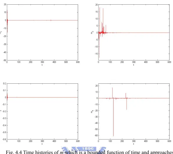
Fig. 4.4 Time histories of m which is a bounded function of time and approaches to zero.
30
Fig. 5.1 Phase portraits of error dynamics for Case I. 39
Fig. 5.3 Time histories of ,
i i
x y for Case I. 39
Fig. 5.4 Phase portrait of error dynamics for Case II. 40
Fig. 5.5 Time histories of errors for Case II. 40
Fig. 5.6 Time histories of 50
i i
x − +y and −Fsinωtcosωt for Case II. 40
Fig. 5.7 Phase portraits of error dynamics for Case III. 41
Fig. 5.8 Time histories of errors for Case III. 41
Fig. 5.9 Time histories of 3 80
10
i
x + and y for Case III. i 41
Fig. 5.10 Phase portrait of error dynamics for Case IV. 42
Fig. 5.11 Time histories of errors for Case IV. 42
Fig. 5.12 Time histories of 150
i i
x− +y and -2
i
z
for Case IV. 42
Fig. 6.1 Chaotic phase portraits for a new Duffing-Van der Pol system in the first quadrant.
52
Fig. 6.2 Phase portrait of error dynamics for Case I. 52
Fig. 6.3 Time histories of errors for Case I. 53
Fig. 6.4 Phase portrait of error dynamics for Case II. 53
Fig. 6.5 Time histories of errors for Case II. 54
Fig. 6.6 Time histories of
i
x for Case II. 54
Fig. 6.7 Phase portrait of error dynamics for Case III. 54
Fig. 6.8 Time histories of errors for Case III. 55
Fig. 6.9 Time histories of
i
x for Case III. 55
Fig. 6.10 Periodic phase portraits for a translated new Duffing-Van der Pol system in the first quadrant.
55
Fig. 6.12 Time histories of errors. 56 Fig. 6.13 Time histories of
i
x . 56
Fig. 7.1 Time histories of
1
L , L , and 1 L . 1 63
Fig. 7.2 The bifurcation diagram for new Duffing-Van der Pol system with Legendre function parameters.
63
Fig. 7.3 The Lyapunov exponents for new Duffing-Van der Pol system with Legendre function parameters.
64
Fig. 7.4 Phase portrait, Poincaré maps, and time histories for new Duffing-Van der Pol system with Legendre function parameters when k=0.35 (period 1).
64
Fig. 7.5 Phase portrait, Poincaré maps, and time histories for new Duffing-Van der Pol system with Legendre function parameters when k=0 (chaos).
65
Fig. 7.6 Phase portraits of error dynamics. 65
Fig. 7.7 Time histories of errors. 66
Fig. A2.1 Partial regions Ω and
1
Chapter 1
Introduction
In the phenomenon of chaos, the chaotic state is very sensitive to its initial condition and chaos causes often irregular behavior in practical systems. Slight errors occurring in initial states of two identical oscillators will lead to completely different trajectories after enough time. Research efforts have studied control and synchronization of chaos in many chaotic systems [1-4].
Many methods have been applied theoretically and experimentally to synchronize chaotic system [5-7]. Chaos synchronization has been widely investigated in a variety of fields such as secure communication [8], biological science [9], chemical reaction [10], physical science [11], and many other fields. So far, there exist many types of synchronization such as complete synchronization [4,12,13], phase synchronization [14,15], lag synchronization [16,17], projective synchronization [18-22], and generalized synchronization [23], etc. Complete synchronizations and antisynchronizations are the special cases of generalized projective synchronization where the scaling factor α = 1 and α = -1 , respectively.
Many approaches for the synchronization of chaotic systems are based on the exact knowledge of the system structure and parameters. But in practice, almost all parameters of the system are uncertain. In current study, the traditional Lyapunov stability theorem and Babalat lemma are used to prove that the error vector approaches zero in adaptive synchronization [24-28]. But the question of that why the estimated parameters also approach uncertain parameters remains unanswered. By the pragmatical asymptotical stability theorem, the question can be answered strictly [29-31].
〝master〞 system and 〝slave〞 system. The final state y of 〝slave〞 system not only depends upon the state x of 〝master〞 system but also depends upon itself. In other words, the 〝slave〞 system does not completely obey the 〝master〞 system but plays a role to determine the final state y of 〝slave〞 system [32]. The generalized synchronization is a special case of the symplectic synchronization. Besides, the state variables of another different order system as a constituent of functional relation between 〝master〞and 〝slave〞are used.
Chaos control has attracted a great deal of attention from various fields. There are many control techniques for chaos control, such as active control [33], observer-based control [34], feedback and non-feedback control [35-38], inverse optimal control [39], adaptive control [40,41], etc. A new chaos synchronization and chaos control strategy by GYC partial region stability theory are proposed [42,43]. By using the GYC partial region stability theory, the controllers are of lower degree than that of controllers by using traditional Lyapunov asymptotical stability theorem [21-28]. The simple linear homogeneous Lyapunov function of error states makes the controllers introducing less simulation error.
This thesis is organized as follows. Chapter 2 gives the dynamic equation of new Duffing-Van der Pol system. The chaotic behaviors are studied. In Chapter 3 and Chapter 4, numerical simulations of generalized and symplectic synchronization scheme based on the pragmatical asymptotical stability theorem with adaptive control and new dynamic surface control are presented. In Chapter 5, numerical simulations of chaos synchronization scheme based on GYC partial region stability theory are presented. In Chapter 6, numerical simulations of chaos control and anti-control scheme based on GYC partial region stability theory are presented. In Chapter 7, numerical simulations of chaos synchronization scheme using chaotic system with Legendre function parameters are presented. In Chapter 8, conclusions are drawn.
Chapter 2
Chaos of a New Duffing-Van der Pol System
In this Chapter, the chaotic behaviors of a new Duffing-Van der Pol system is studied numerically by phase portraits, time histories, Poincaré maps, Lyapunov exponents, bifurcation diagrams, and parametric diagram.
2.1 Description of New Duffing-Van der Pol System
Duffing equation and Van der Pol equation are two typical nonlinear nonautonomous systems: 1 2 3 2 1 1 2 sin dx x dt dx x x ax d t dt ω ⎧ = ⎪⎪ ⎨ ⎪ = − − − + ⎪⎩ (2.1)
(
)
3 4 2 4 3 1 3 4 sin dx x dt dx bx c x x f t dt ω ⎧ = ⎪⎪ ⎨ ⎪ = − + − + ⎪⎩ (2.2)A new autonomous Duffing-Van der Pol system is proposed by coupling of these two typical nonautonomous systems. Exchanging sinωt in Eq. (2.1) with x3 and
sinωt in Eq. (2.2) with x1, we obtain the new autonomous Duffing-van der Pol
system:
(
)
1 2 3 2 1 1 2 3 3 4 2 4 3 1 3 4 1 dx x dt dx x x ax dx dt dx x dt dx bx c x x fx dt ⎧ = ⎪ ⎪ ⎪ = − − − + ⎪ ⎨ ⎪ = ⎪ ⎪ ⎪ = − + − + ⎩ (2.3)follows.
2.2 Computational Analysis of a New Duffing-Van der Pol
System
For numerical analysis of computation, this system exhibits chaos when the parameters of system are a=0.01,b=1,c=5,d =0.67, f =0.05 and the initial states of system are x1(0) 2, (0) 2.4, (0) 5, (0) 6= x2 = x3 = x4 = . The bifurcation diagram by
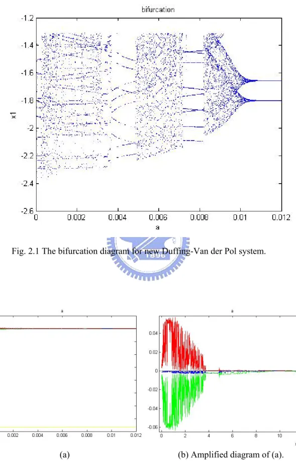
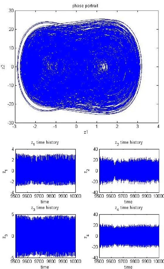
changing damping parameter a is shown in Fig. 2.1. Its corresponding Lyapunov exponents are shown in Fig. 2.2. The phase portraits, time histories, and Poincaré maps of the systems are showed in Fig. 2.3~Fig. 2.5. When a=0.012, period 2 phenomena are shown in Fig. 2.3. When a=0.01 and a=0.0006, the chaotic behaviors are given in Fig. 2.4 and Fig. 2.5, respectively. In addition, the parametric diagram is obtained in Fig. 2.6.
Fig. 2.1 The bifurcation diagram for new Duffing-Van der Pol system.
(a) (b) Amplified diagram of (a). Fig. 2.2 The Lyapunov exponents for new Duffing-Van der Pol system.
Fig. 2.3 Phase portrait, Poincaré maps, and time histories for new Duffing-Van der Pol system with a=0.012 (period 2).
Fig. 2.4 Phase portrait, Poincaré maps, and time histories for new Duffing-Van der Pol system with a=0.01 (chaos).
Fig. 2.5 Phase portrait, Poincaré maps, and time histories for new Duffing-Van der Pol system with a=0.0006 (chaos).
Fig. 2.6 The parametric diagram for new Duffing-Van der Pol system with b=1,
Chapter 3
Pragmatical Hybrid Projective Chaotic Generalized
Synchronization of Chaotic System with Uncertain
Parameters by Adaptive Control
A new kind of generalized synchronization, pragmatical hybrid projective
chaotic generalized synchronization (PHPCGS) of two identical chaotic systems of
which one has uncertain parameters, by pragmatical adaptive control, is achieved with the state vector of another hyperchaotic chaotic system as a constituent of the functional relation between master and slave. The PHPCGS is as follows:
( ) y G x= =zH x (3.1) where n 1 2 1 2 ( , ,..., ) ,T ( , ,..., )T R n n
x= x x x y= y y y ∈ are the n-dimensional state
vectors of master system and slave system, respectively,
[
]
( )1, ,...,2
n n n
H =diag h h h ∈R × is a constant scaling diagonal matrix where
i
h are
called scaling factors, which may either positive or negative to form the hybrid projective synchronization. z=
[
z ( ), ( ),..., ( )1 t z t2 z tn]
is a given state vector withchaotic time function components. The existence of z causes so called chaotic synchronization. Based on the pragmatical asymptotical stability theorem, adaptive control law is used. Furthermore, the scheme can achieve not only projective synchronization, but also projective anti-synchronization. With all above consideration, PHPCGS is achieved. Numerical simulations are provided to verify the effectiveness of the proposed scheme.
3.1 The PHPCGS Scheme of Chaotic Systems by Adaptive
Control
controls the slave system. The master system is given by ( , ) x=Ax+ f x B (3.2) where [ , ,1 2 ] T n n
x= x x x ∈R denotes a state vector, A is an n n× uncertain
constant coefficient matrix, f is a nonlinear vector function, and B is a vector of uncertain constant coefficients in f. The slave system is given by
ˆ ( , )ˆ ( )
y=Ay+ f y B +u t (3.3)
where [ , ,1 2 ]
T n n
y= y y y ∈R denotes a state vector, ˆA is an n n× estimated
coefficient matrix, ˆB is a vector of estimated coefficients in f, and
1 2
( ) [ ( ), ( ), ( )]T n n
u t = u t u t u t ∈R is a control input vector. The chaotic system which affords chaotic z matrix, is called functional system because in Eq. (3.1), it is a constituent of function G. The functional system is given by
( )
z Cz g z= + (3.4)
where [ , ,1 2 ]
T n n
z= z z z ∈R denotes a state vector, C is an n n× constant
coefficient matrix, g is a nonlinear vector function. PHPCGS demands:
( , z) z
y = G x = H x (3.5) Our goal is to accomplish Eq. (3.5) via controller u(t) and parameter update dynamics. Define the error vector e:
z -
e = H x y (3.6) The synchronization is achieved when
(
)
lim i 0 1, 2,...,
t→∞e = i= n (3.7)
By (3.2), (3.3), and (3.4), the error dynamics is
( )
ˆ ˆ - ( , ) - ( , ) - ( ) e zHx zHx y zHAx A y zHf x B f y B CzHx g z Hx u t = + − = + + + (3.8)A Lyapunov function V e A B( , c, c) is chosen as a positive definite function of , c, c e A B : c T c c T c T c c B e e A A B B A e V ~ ~ 2 1 ~ ~ 2 1 2 1 ) ~ , ~ , ( = + + (3.9)
where A A A= − ˆ, B B B= − ˆ, Ac and Bc are two vectors whose elements are all
the elements of matrix A and of matrix B , respectively. By properly choosing
( )
,u t Ac, and Bc, its time derivative V along any solution of Eq. (3.8) and
parameter update differential equations for Ac and Bc can be obtained as T
V =e Ce (3.10) where C is a diagonal negative definite matrix. V is a negative definite function of e but a negative semi-definite function of e A B, c, c. In the current scheme of adaptive synchronization [24-28], the traditional Lyapunov stability theorem and Babalat lemma are used to prove that the error vector approaches zero, as time approaches infinity. But the question that why the estimated parameters also approach uncertain parameters remains unanswered. By the GYC pragmatical asymptotical stability theorem, the question can be answered strictly. The equilibrium point e A B= = = 0 is pragmatically asymptotically stable. Under the assumption of equal probability, it is actually asymptotically stable, as shown in Appendix. Hence, PHPCGS can be achieved.
3.2 Description of Two New Chaotic 4D Systems, a New
Duffing-Van der Pol System and a New Mathieu-Duffing
System
This section introduces new Duffing-Van der Pol system and new Mathieu-Duffing system.
3.2.1 New Duffing-Van der Pol system
The master new Duffing-Van der Pol system:
(
)
1 2 3 2 1 1 2 3 3 4 2 4 3 1 3 4 1 dx x dt dx x x ax dx dt dx x dt dx bx c x x fx dt ⎧ = ⎪ ⎪ ⎪ = − − − + ⎪ ⎨ ⎪ = ⎪ ⎪ ⎪ = − + − + ⎩ (3.11)The slave system is
(
)
1 2 1 3 2 1 1 2 3 2 3 4 3 2 4 3 3 4 1 4 ˆ ˆ ˆ ˆ 1 ˆ dy y u dt dy y y ay dy u dt dy y u dt dy by c y y fy u dt ⎧ = + ⎪ ⎪ ⎪ = − − − + + ⎪ ⎨ ⎪ = + ⎪ ⎪ ⎪ = − + − + + ⎩ (3.12)where u u u1, , ,2 3 u are control inputs, a, b, c, d, f are uncertain parameters, 4
ˆ ˆ ˆ, , ˆ,
a b c d and ˆf are estimated parameters. The master system exhibits chaos when the parameters are a=0.01,b=1,c=5, d =0.67, f =0.05and the initial states are x1(0) 2, (0) 2.4, (0) 5,= x2 = x3 = x4(0) 6= .
3.2.2 New Mathieu-Duffing system
The functional system is a new Mathieu-Duffing system. By coupling two noautonomous nonlinear Mathieu system and Duffing system, a new Mathieu-Duffing system is obtained:
(
)
(
)
1 2 3 2 3 3 3 1 3 3 3 1 3 2 3 3 3 4 3 4 3 3 3 4 3 1 dz z dt dz a b z z a b z z c z d z dt dz z dt dz z z f z g z dt ⎧ = ⎪ ⎪ ⎪ = − + − + − + ⎪ ⎨ ⎪ = ⎪ ⎪ ⎪ = − − − + ⎩ (3.13)3
b =0.597 ,c =0.005,3 d =-24.44 ,3 f =0.002 ,3 g =14.63 and the initial states of system 3 are z (0)=-2 ,1 z (0)=10 ,2 z (0)=-2 ,3 z (0)=10 , its phase portraits and time histories as 4 shown in Fig. 3.1.
3.3 Numerical Results for PHPCGS of Two New
Duffing-Van der Pol Systems
Since the master system, slave system, and functional system are described by Eq. (3.11), Eq. (3.12), and Eq. (3.13), respectively, the error dynamics Eq. (3.8) becomes:
(
)
(
)
(
)
{
}
(
)
(
)
{
}
(
)
1 1 2 1 1 2 2 1 3 3 2 2 2 1 1 2 3 2 3 3 3 1 1 3 2 3 3 3 1 1 2 3 2 3 3 4 3 3 4 4 3 2 3 4 4 4 3 3 4 1 4 3 3 3 4 3 1 2 3 3 4 1 4 ˆ ˆ 1 ˆ ˆ 1 ˆ e h x z x z y u e h z x x ax dx x a b z z z c z d z y y ay dy u e h x z x z y u e h z bx c x x fx x z z f z g z by c y y fy u = + − − ⎧ ⎪ ⎡ ⎤ ⎪ = ⎣⎡− − − + ⎤⎦+ ⎣− + + − + ⎦ + + + − − ⎨ = + − − ⎡ ⎤ ⎡ ⎤ = ⎣− + − + ⎦+ ⎣− − − + ⎦ + − − − − ⎪ ⎪⎪ ⎪ ⎪ ⎪ ⎪ ⎪⎩ (3.14)Choose a positive definite Lyapunov function for e1, e2, e3, e4, a b c d, , , , f :
2 2 2 2 2 2 2 2 2 1 2 3 4 1 ( ) 2 V = e +e +e +e +a +b +c +d + f (3.15) where a a a= − ˆ, b b b= − ˆ, c c c= − ˆ, d = −d dˆ, and f = −f fˆ . Controllers and parameter update dynamics are selected as:
(
)
(
)
(
)
{
}
(
)
(
)
{
}
(
)
1 1 2 1 1 2 2 1 3 3 2 2 2 1 1 2 3 2 3 3 3 1 1 3 2 3 3 3 1 1 2 3 2 3 3 4 3 3 4 4 3 2 3 4 4 4 3 3 4 1 4 3 3 3 4 3 1 2 3 3 4 1 4 ˆ ˆ ˆ ˆ 1 ˆ ˆ 1 ˆ u h x z x z y e u h z x x ax dx x a b z z z c z d z y y ay dy e u h x z x z y e u h z bx c x x fx x z z f z g z by c y y fy e = + − + ⎧ ⎪ ⎡ ⎤ ⎡ ⎤ ⎪ = − ⎣ + + − ⎦− ⎣ + + + − ⎦ ⎪ ⎪ + + + − + ⎪ ⎨ = + − + ⎡ ⎤ ⎡ ⎤ = ⎣− + − + ⎦+ ⎣− − − + ⎦ + − − − + ⎪ ⎪ ⎪ ⎪ ⎪⎩ (3.16)(
)
2 2 2 2 4 4 4 3 2 4 4 4 3 4 2 2 2 3 4 4 4 1 ˆ ˆ ˆ 1 ˆ ˆ a e h z x b e h z x c e h z x x d e h z x f e h z x ⎧ = − ⎪ ⎪ = − ⎪ ⎪ = − ⎨ ⎪ ⎪ = ⎪ ⎪ = ⎩ (3.17)The time derivative of V is
2 2 2 2
1 2 3 4 0
V = − −e e −e −e ≤ (3.18) which is negative semi-definite function for e1, e2, e3, e4, a b c d, , , , f . The Lyapunov asymptotical stability theorem cannot be satisfied in this case. The common origin of error dynamics and parameter update dynamics cannot be concluded to be asymptotically stable. By pragmatical asymptotical theorem, D is a 9-manifold, n = 9 and the number of error state variables p = 4. Whene = 1 e = 2 e = 3 e = 0 and 4
a
,b , c , d , f take arbitrary values , V =0, so X is a 5-manifold, m = n - p = 9 – 4 = 5. m + 1 < n are satisfied. By the pragmatical asymptotical stability theorem, the common origin of error dynamics (3.14) and parameter dynamics (3.17) is asymptotically stable. The equilibrium point e = 1 e = 2 e = 3 e = a = b = c 4
= d = f = 0 is pragmatically asymptotically stable. The PHPCGS is achieved under this scheme.
In this numerical simulation, we select the “unknown” parameter and initial states of the master system and of functional system the same as that in Section 3.2 to ensure the chaotic behavior. The initial states of slave system are y1
( )
0 = y2( )
0 =5and y3
( )
0 = y4( )
0 =10 , the estimated parameters have initial conditions( ) ( ) ( )
ˆ ˆ( )
ˆ( )
ˆ 0 0 ˆ 0 0 0 0
a =b =c =d = f = and the scaling matrix is
1 1 (2, , 2, )
2 2
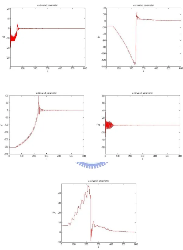
Fig. 3.3 Time histories of the differences of uncertain parameters and estimated parameters.
Chapter 4
Pragmatical Chaotic Symplectic Synchronization
with Different Order System by New Dynamic
Surface Control
A new type of chaotic synchronization, pragmatical chaotic symplectic
synchronization (PCSS), is obtained with the state variables of another different order
system as a constituent of the functional relation between 〝master〞 and 〝slave〞. The PCSS as follows:
(
, ,)
( )
y H x y t= +F t (4.1) where x and y are the 〝master〞 and the 〝slave〞 system, respectively. The final state y of 〝slave〞 system not only depends upon the state x of 〝master〞 system but also depends upon itself. In other words, the 〝slave〞 system does not completely obey the 〝master〞 system but plays a role to determine the final state y of 〝slave〞 system. This kind of synchronization called “symplectic synchronization”*, and the 〝master〞 and 〝slave〞 system called partner A and partner B, respectively. When
H=H(x,t) symplectic synchronization becomes traditional generalized synchronization.
Therefore the latter is a special case of the former.
* The term ‘‘symplectic’’ comes from the Greek for ‘‘intertwined’’. H. Weyl first introduced the term in 1939 in his book “The Classical Groups”(P. 165 in both the first edition, 1939, and second edition, 1946, Princeton University Press)
( )
F t is a given chaotic vector of time from the states of another different order
chaotic system. Based on the pragmatical asymptotical stability theorem, new dynamic surface control (NDSC) which makes the controllers more simple, and adaptive control, the synchronization is achieved. Numerical simulations are provided to verify the effectiveness of the proposed scheme.
4.1 Pragmatical Chaotic Symplectic Synchronization Scheme
There are two identical nonlinear chaotic dynamical systems, and the 〝master 〞 system controls the 〝slave〞 system. In symplectic synchronization, the 〝master〞 system is called partner A:
( , )
x=Ax+ f x B (4.2)
where [ , ,1 2 ]
T n n
x= x x x ∈R denotes a state vector, A is an n n× uncertain
constant coefficient matrix, f is a nonlinear vector function, and B is a vector of uncertain constant coefficients in f. The 〝slave〞 system is called partner B:
ˆ ( , )ˆ
y= Ay+ f y B (4.3)
where [ , ,1 2 ]
T n n
y= y y y ∈R denotes a state vector, ˆA is an n n× estimated
coefficient matrix, ˆB is a vector of estimated coefficients in f. With controllers, partner B becomes ˆ ( , )ˆ ( ) u y =Ay f y B+ +u t (4.4) where ( ) [ ( ), ( ),1 2 ( )] T n n
u t = u t u t u t ∈R is a control input vector. The chaotic system which affords chaotic F(t) vector, is called functional system. However, the PCSS also can be achieved even the order of functional system is different from that of partners A and B. Now we choose the order of the former is less than the latter. The augmented functional system can be easily obtained as shown in Section 4.3. The
augmented functional system becomes ( ) F =CF g F+ (4.5) where [ , ,1 2 ] T n n
F = F F F ∈R denotes a state vector, C is an n n× constant
coefficient matrix, g is a nonlinear vector function. PCSS demands:
(
, ,)
( )
y H x y t= +F t
(4.6)
where H x y t consists of state vector x of partner A and state vector y of partner
(
, ,)
B. Our goal is to accomplish Eq. (4.6) via controller u(t) and parameter update dynamics. Define the error vector e:(
)
( )
, , u
e =H x y t −y +F t (4.7) The synchronization is achieved when
(
)
lim i 0 1, 2,...,
t→∞e = i= n (4.8)
The error dynamics is
( ) u H H H e x y y F t x y t ∂ ∂ ∂ = + + − + ∂ ∂ ∂ (4.9)
By Eq. (4.2) ~ Eq. (4.5), Eq. (4.9) becomes
(
)
( )
( )
( )
( )
ˆ ˆ , , ˆ , ˆ H H H e Ax f x B Ay f y B x y t Ay f y B u t CF g F ∂ ∂ ⎡ ⎤ ∂ = ⎡⎣ + ⎤⎦+ ⎣ + ⎦+ ∂ ∂ ∂ − − − + + (4.10)In order to reduce terms of the u(t), NDSC is used which makes u(t) more simple. This method extends the traditional dynamic surface control [44]. A virtual controller
W is chosen as follows
( )
( , , ) ( ), lim ( , , ) ( ) t mW W H x y t F t W t H x y t F t →∞ + = + = + (4.11)( , , ) ( ) s W H x y t= − +F t (4.12) Its derivative is
(
( , , ) ( ))
s d s H x y t F t m dt − = − + (4.13) Eq. (4.7) and Eq. (4.10) becomesu
e =W y− (4.14)
( )
( )
ˆ , ˆ
e W= −Ay− f y B −u t (4.15) A Lyapunov function V e s A B( , , c, c) is chosen as a positive definite function of
, , c, c e s A B : 1 1 1 1 ( , , , ) 2 2 2 2 T T T T c c c c c c V e s A B = e e+ s s+ A A + B B (4.16) where A A A= − ˆ, B B B= − ˆ, Ac and Bc are two vectors whose elements are all
the elements of matrix A and of matrix B , respectively. Its time derivative along any solution of Eq. (4.13) and Eq. (4.15) and parameter update differential equations for Ac and Bc is V . Choose u(t), m(t), Ac and Bc so that
T T
V =e Pe s Qs+ (4.17) where P and Q are diagonal negative definite matrixes, and V is a negative semi-definite function of e s A B, , c, c . In the current scheme of adaptive synchronization [24-28], the traditional Lyapunov stability theorem and Babalat lemma are used to prove that the error vector approaches zero, as time approaches infinity. But the question that why the estimated parameters also approach uncertain parameters remains unanswered. By the pragmatical asymptotical stability theorem, the question can be answered strictly. The equilibrium point e s A B= = = = is 0 pragmatically asymptotically stable (see Appendix). Under the assumption of equal
probability, it is actually asymptotically stable. Hence, the PCSS can be achieved.
4.2 Numerical Results for the PCSS by New Dynamic
Surface Control
Since the partner A, new Duffing-Van der Pol system, is described as
(
)
1 2 3 2 1 1 2 3 3 4 2 4 3 1 3 4 1 dx x dt dx x x ax dx dt dx x dt dx bx c x x fx dt ⎧ = ⎪ ⎪ ⎪ = − − − + ⎪ ⎨ ⎪ = ⎪ ⎪ ⎪ = − + − + ⎩ (4.18)where a, b, c, d, f are uncertain parameters. The partner B is described as
(
)
1 2 3 2 1 1 2 3 3 4 2 4 3 3 4 1 ˆ ˆ ˆ ˆ 1 ˆ dy y dt dy y y ay dy dt dy y dt dy by c y y fy dt ⎧ = ⎪ ⎪ ⎪ = − − − + ⎪ ⎨ ⎪ = ⎪ ⎪ ⎪ = − + − + ⎩ (4.19)where a b c dˆ, ˆ, ˆ, ˆ and ˆf are estimated parameters.
For this scheme, u1, u2, u3 and u4 are added to the partner B then becomes
controlled partner B:
(
)
1 2 1 3 2 1 1 2 3 2 3 4 3 2 4 3 3 4 1 4 ˆ ˆ ˆ ˆ 1 ˆ dy y u dt dy y y ay dy u dt dy y u dt dy by c y y fy u dt ⎧ = + ⎪ ⎪ ⎪ = − − − + + ⎪ ⎨ ⎪ = + ⎪ ⎪ ⎪ = − + − + + ⎩ (4.20)variable is 2 4 1 z =z :
(
)
(
)
1 2 1 2 1 3 2 3 1 2 3 4 1 2 1 2 dz g z z dt dz z z hz dt dz z z kz dt dz gz z z dt ⎧ = − ⎪ ⎪ ⎪ = − + ⎪ ⎨ ⎪ = − ⎪ ⎪ ⎪ = − ⎩ (4.21)In the PCSS, we select the
(
) ( )
1, 2, , , , 2, 3, j j i i i i i n H x y t x y z i even j i odd = ⎧ ⎪ = − + ⎨ = ⎨⎧ = ⎪ = ⎩ ⎩ (4.22) Now n=4. By NDSC, the error dynamics Eq. (4.15) becomes:(
)
1 1 2 1 3 2 2 1 1 2 3 2 3 3 4 3 2 4 4 3 3 4 1 4 ˆ ˆ ˆ ˆ 1 ˆ e W y u e W y y ay dy u e W y u e W by c y y fy u ⎧ = − − ⎪ = + + + − − ⎪ ⎨ = − − ⎪ ⎪ = + − − − − ⎩ (4.23)and the boundary layer error dynamics Eq. (4.13) becomes:
(
)
(
)
(
)
(
)
(
)
(
)
(
)
2 3 2 1 1 1 2 1 1 2 1 2 1 1 3 2 3 2 2 2 2 1 1 2 3 2 1 1 2 3 2 2 1 3 2 2 3 2 3 3 3 4 3 3 4 3 1 2 3 3 2 2 4 4 4 4 3 3 4 1 4 3 3 4 3 3 ˆ ˆ 2 2 3 3 ˆ ˆ 2 1 1 s s x x y x y gz z z m s s x y x x ax dx x y y ay dy m z z z hz s s x x y x y z z z kz m s s x y bx c x x fx x by c y m − ⎡ ⎤ = − −⎣ − + − ⎦ − ⎡ = − −⎣ − − − + − − − − + + − + ⎤⎦ − ⎡ ⎤ = − −⎣ − + − ⎦ − = − − − + − + −(
− +(
−)
)
(
)
2 4 1 1 4 2 1 ˆ 4 y fy gz z z z ⎧ ⎪ ⎪ ⎪ ⎪ ⎪ ⎪⎪ ⎨ ⎪ ⎪ ⎪ ⎪ ⎡ + ⎣ ⎪ ⎪ + − ⎤ ⎪ ⎦ ⎩ (4.24)Choose a positive definite Lyapunov function for e1, e2, e3, e4, s1, s2, s3, s 4,
, , , , a b c d f : 2 2 2 2 2 2 2 2 2 2 2 2 2 1 2 3 4 1 2 3 4 1 ( ) 2 V = e +e +e +e + + + + +s s s s a +b +c +d + f (4.25) where a=(a a− ˆ), b~=(b−bˆ), ~c =(c−cˆ), d~=(d−dˆ), and ~f = (f − fˆ). We
select controllers, estimated parameter dynamics, and the m as:
(
)
1 1 2 1 3 2 2 1 1 2 3 2 3 3 4 3 2 4 4 3 3 4 1 4 ˆ ˆ ˆ ˆ 1 ˆ u W y e u W y y ay dy e u W y e u W by c y y fy e ⎧ = − + ⎪ = + + + − + ⎪ ⎨ = − + ⎪ ⎪ = + − − − + ⎩ (4.26)They are more simple.
(
)
2 2 2 2 3 4 4 4 2 2 4 4 3 4 2 3 2 2 1 4 4 4 ˆ 2 ˆ 2 ˆ 2 1 ˆ 2 ˆ 2 a x y s b x x y s c x y x s d x x y s f x x y s ⎧ = − ⎪ ⎪ = − ⎪ ⎪ = − ⎨ ⎪ ⎪ = ⎪ ⎪ = ⎩ (4.27)(
)
(
) (
)
(
)
(
)
( )
(
)
(
( )
)
1 1 2 3 2 1 1 2 1 1 2 1 2 1 2 2 3 2 3 2 2 2 1 1 2 3 2 1 1 2 3 2 1 3 2 3 3 2 3 2 3 3 4 3 3 4 3 1 2 3 4 4 2 2 2 4 4 4 3 3 4 1 4 3 3 4 1 3 3 ˆ ˆ ˆ ˆ 2 2 3 3 ˆ ˆ ˆ ˆ ˆ ˆ 2 1 1 4 s m s x x y x y gz z z s m s x y x x ax dx x y y ay dy z z z hz s m s x x y x y z z z kz s m s x y bx c x x fx x by c y y fy g − = − − − + − − = − − − − − + − − − − + + − + − = − − − + − − = − − − + − + − − + − + + z z z z1 4(
2 1)
⎧ ⎪ ⎪ ⎪ ⎪ ⎪⎪ ⎨ ⎪ ⎪ ⎪ ⎪ ⎪ − ⎪⎩ (4.28)The time derivative of V is
2 2 2 2 2 2 2 2
1 2 3 4 1 2 3 4 0
V = − −e e −e −e −s −s −s −s ≤ (4.29) which is negative semi-definite function for e1, e2, e3, e4, s1, s2, s3, s4, a ,
, , ,
b c d f . The Lyapunov asymptotical stability theorem cannot be satisfied in this case. The common origin of error dynamics, parameter update dynamics, and boundary layer error dynamics cannot be concluded to be asymptotically stable. By pragmatical asymptotical theorem, D is a 13-manifold, n = 13 and the number of error state variables p = 8. When e = 1 e = 2 e = 3 e = 4 s = 1 s = 2 s = 3 s = 0 and 4
a
,b , c , d , f take arbitrary values , V =0, so X is a 5-manifold, m = n - p = 13 – 8 = 5. m + 1 < n are satisfied. By the pragmatical asymptotical stability theorem, the common origin of error dynamics (4.23), boundary layer error dynamics (4.24), and parameter dynamics (4.27) are asymptotically stable. The equilibrium point e = 1 e 2
= e = 3 e = 4 s = 1 s = 2 s = 3 s = a = b = c = d = 4 f = 0 is pragmatically asymptotically stable. The PCSS is achieved under this scheme.
In this numerical simulation, we select the “unknown” parameter and initial states of the partner A and of functional system as a=0.01, b=1, c=5, d=0.67, f=0.05,
g=36, h=20, k=3 to ensure the chaotic behavior. The initial states of those system are
( )
( )
( )
( )
( )
( )
( )
1 0 2, 2 0 2.4, 3 0 5, 4 0 6, 1 0 5, 2 0 5, 3 0 10,
x = x = x = x = y = y = y =
( )
( )
( )
( )
( )
4 0 10, 1 0 2 0 3 0 4 0 10
y = z =z =z =z = . The estimated parameters have initial
conditions aˆ
( )
0 =bˆ( ) ( )
0 =cˆ 0 =dˆ( )
0 = fˆ( )
0 =0. The numerical results are shown in Fig. 4.1 ~ Fig. 4.4.Fig. 4.2 Time histories of the differences of uncertain parameters and estimated parameters.
Fig. 4.4 Time histories of m which is a bounded function of time and approaches to zero.
Chapter 5
Chaos Generalized Synchronization of New
Duffing-Van der Pol Systems by GYC Partial Region
Stability Theory
A new chaos generalized synchronization strategy, using the GYC partial region stability theory, the controllers are of lower degree than that of controllers by using traditional Lyapunov asymptotical stability theorem. The simple linear homogeneous Lyapunov function of error states makes the controllers introducing less simulation error. A new Duffing-Van der Pol system and hyper-chaotic Lü system [46] are used as simulated examples.
5.1 Chaos Generalized Synchronization Strategy
Consider the following unidirectional coupled chaotic systems ( , ) ( , ) t t = = + x f x y h y u (5.1) where
[
1, , ,2]
T n n x x x R = ∈ x ,[
1, , ,2]
T n n y y y R = ∈y denote the master state
vector and slave state vector respectively, f and h are nonlinear vector functions, and
[
1, , ,2]
T nn
u u u R
= ∈
u is a control input vector.
The generalized synchronization can be accomplished when t→ ∞ , the limit of the error vector
[
1, , ,2]
T n e e e = e approaches zero: lim 0 t→∞e= (5.2) where ( ) = − e G x y (5.3) ) ( x G is a given function of x .
By using the partial region stability theory (see Appendix), the linear homogeneous terms of the entries of e can be used to construct a positive definite Lyapunov function and the controllers can be designed in lower degree.
5.2 Numerical Simulations
Two new Duffing-Van der Pol systems with unidirectional coupling are given:
(
)
1 2 3 2 1 1 2 3 3 4 2 4 3 1 3 4 1 x x x x x ax dx x x x bx c x x fx = ⎧ ⎪ = − − − + ⎪ ⎨ = ⎪ ⎪ = − + − + ⎩(
)
1 2 1 3 2 1 1 2 3 2 3 4 3 2 4 3 1 3 4 1 4 y y u y y y ay dy u y y u y by c y y fy u = + ⎧ ⎪ = − − − + + ⎪ ⎨ = + ⎪ ⎪ = − + − + + ⎩ (5.4)CASE I. The generalized synchronization error function is
30, 1, 2, 3, 4
i i i
e = − +x y i= (5.5) The addition of the constant 30 makes the error dynamics always happens in the first quadrant. Our goal is yi = +xi 30, i.e.
limt→∞ei =lim(t→∞ xi− +yi 30) 0,= i=1, 2, 3, 4 (5.6)
The error dynamics becomes
(
)
(
(
)
)
2 2 1 1 1 2 2 1 1 1 3 3 2 2 2 2 2 1 1 2 3 1 1 2 3 1 1 2 2 2 3 3 3 4 4 3 3 3 2 2 2 2 4 4 4 3 3 4 1 3 3 4 1 3 3 4 ( ) 1 1 e x y x y x x u e x y x x ax dx y y ay dy x x u e x y x y x x u e x y bx c x x fx by c y y fy x x u ⎧ = − = − + − − ⎪ = − = − − − + − − − − + + − − ⎪ ⎨ = − = − + − − ⎪ ⎪ = − = − + − + − − + − + + − − ⎩ (5.7)Let initial states be ( , , , )x x x x = (2, 2.4, 5, 6), 1 2 3 4 ( ,y y y y = (5, 5, 1, 1) and 1 2, 3, )4 system parameters a=0.01, b=1, c=5, d =0.67, f =0.05, we find that the error
dynamic always exists in first quadrant as shown in Fig. 5.1. By GYC partial region asymptotical stability theory, one can choose a Lyapunov function in the form of a positive definite function in first quadrant:
1 2 3 4
V = + + + (5.8) e e e e
Its time derivative is
(
)
(
)
(
)
(
)
(
)
(
)
1 2 3 4 2 2 2 2 1 1 1 3 3 2 2 1 1 2 3 1 1 2 3 1 1 2 2 2 4 4 3 3 3 2 2 2 2 3 1 3 4 1 3 1 3 4 1 3 3 4 V e e e e x y x x u x x ax dx y y ay dy x x u x y x x u bx c x x fx by c y y fy x x u = + + + = − + − − + − − − + + + + − + − − + − + − − + − + − + + − − − + − − (5.9) Choose(
)
(
)
2 1 2 2 1 1 3 3 2 2 1 1 2 3 1 1 2 3 1 2 2 3 4 4 3 3 2 2 2 4 3 1 3 4 1 3 1 3 4 1 3 4 u x y x e u x x ax dx y y ay dy x e u x y x e u bx c x x fx by c y y fy x e ⎧ = − + + ⎪ = − − − + + + + − − + ⎪ ⎨ = − + + ⎪ ⎪ = − + − + + − − − − + ⎩ (5.10) We obtain 1 2 3 4 0 V = − − − − <e e e e (5.11) which is negative definite function in the first quadrant. Four state errors versus time and time histories of states are shown in Fig. 5.2 and Fig. 5.3.CASE II. The generalized synchronization error function is
sin cos 50, 1, 2, 3, 4
i i i
e = − +x y F ωt ωt+ i= (5.12)
Our goal is yi = +xi Fsinωtcosωt+50, i.e.
limt→∞ei =lim(t→∞ xi− +yi Fsinωtcosωt+50) 0,= i=1, 2, 3, 4 (5.13)
2 2 cos sin i i i e = − +x y Fω ωt F− ω ωt
(
)
(
)
(
)
2 2 2 2 1 2 2 2 2 1 3 2 2 2 1 1 2 3 3 2 2 1 1 2 3 2 2 2 2 2 2 2 3 4 4 4 4 3 2 2 2 4 3 3 4 1 2 3 3 4 1 cos sin cos sin ( ) cos sin 1 cos sin 1 e x F t F t y x x u e x x ax dx F t F t y y ay dy x x u e x F t F t y x x u e bx c x x fx F t F t by c y y fy ω ω ω ω ω ω ω ω ω ω ω ω ω ω ω ω = + − − + − − = − − − + + − − − − − + + − − = + − − + − − = − + − + + − − − + − + + 2 2 4 4 4 x x u ⎧ ⎪ ⎪ ⎪ ⎪ ⎨ ⎪ ⎪ ⎪ ⎪ − − ⎩ (5.14)Let initial states be ( , , , )x x x x = (2, 2.4, 5, 6), 1 2 3 4 ( ,y y y y = (5, 5, 1, 1) and 1 2, 3, )4 system parametersa=0.01, b=1, c=5, d =0.67, f =0.05,F = and 5 ω=0.2, we find that the error dynamics always exists in first quadrant as shown in Fig. 5.4. By GYC partial region asymptotical stability theory, one can choose a Lyapunov function in the form of a positive definite function in first quadrant:
1 2 3 4
V = + + + (5.15) e e e e
Its time derivative is
(
)
(
)
(
)
(
)
(
(
)
)
2 2 2 2 2 2 2 2 1 3 2 2 3 2 2 1 1 2 3 1 1 2 3 2 2 2 2 2 2 2 4 4 4 4 3 2 2 2 3 3 4 1 3 2 2 2 3 4 1 4 4 4 cos sin cos sin cos sin 1 cos sin 1 V x F t F t y x x u x x ax dx F t F t y y ay dy x x u x F t F t y x x u bx c x x fx F t F t by c y y fy x x u ω ω ω ω ω ω ω ω ω ω ω ω ω ω ω ω = + − − + − − + + − − − + + − + + + − + − − + + − − + − − + − + − + + − + − − − + − − (5.16) Choose(
)
(
)
2 2 2 1 2 2 2 1 3 2 2 3 2 2 1 1 2 3 1 1 2 3 2 2 2 2 2 3 4 4 4 3 2 2 2 4 3 3 4 1 3 2 2 3 4 1 4 4 cos sin cos sin cos sin 1 cos sin 1 u x F t F t y x e u x x ax dx F t F t y y ay dy x e u x F t F t y x e u bx c x x fx F t F t by c y y fy x e ω ω ω ω ω ω ω ω ω ω ω ω ω ω ω ω ⎧ = + − − + + ⎪ ⎪ = − − − + + − + + + − − + ⎪⎪ = + − − + + ⎨ ⎪ =− + − + + − + ⎪ ⎪ − − − − + ⎪⎩ (5.17) We obtain1 2 3 4 0
V = − − − − <e e e e (5.18) which is negative definite function in first quadrant. Four state errors versus time and time histories of states are shown in Fig. 5.5 and Fig. 5.6.
CASE III. The generalized synchronization error function is
3 1 80, 1, 2, 3, 4 10 i i i e = x − +y i= (5.19) Our goal is 1 3 80 10 i i y = x + , i.e. 3 1 lim lim( 80) 0, 1, 2,3, 4 10 i i i t→∞e =t→∞ x − +y = i= (5.20)
The error dynamics become
2 3 10 i i i i e = x x − y
(
) (
)
(
)
(
)
(
(
)
)
2 2 2 1 1 2 2 1 1 1 2 3 3 2 2 2 2 1 1 2 3 1 1 2 3 1 1 2 2 2 2 3 3 4 4 3 3 3 2 2 2 2 2 4 4 3 3 4 1 3 3 4 1 3 3 4 3 10 3 10 3 10 3 1 1 10 e x x y x x u e x x x ax dx y y ay dy x x u e x x y x x u e x bx c x x fx by c y y fy x x u ⎧ = − + − − ⎪ ⎪ ⎪ = − − − + − − − − + + − − ⎪ ⎨ ⎪ = − + − − ⎪ ⎪ ⎪ = − + − + − − + − + + − − ⎩ (5.21)Let initial states be ( , , , )x x x x = (2, 2.4, 5, 6), 1 2 3 4 ( ,y y y y = (5, 5, 1, 1) and 1 2, , )3 4 system parametersa=0.01, b=1, c=5, d =0.67, f =0.05, we find the error dynamics always exists in first quadrant as shown in Fig. 5.7. By GYC partial region asymptotical stability theory, one can choose a Lyapunov function in the form of a positive definite function in first quadrant:
1 2 3 4
V = + + + (5.22) e e e e
(
)
(
)
(
)
(
)
2 2 2 1 2 2 1 1 1 2 3 3 2 2 2 1 1 2 3 1 1 2 3 1 1 2 2 2 2 3 4 4 3 3 3 2 2 2 2 2 4 3 3 4 1 3 3 4 1 3 3 4 3 10 3 10 3 10 3 1 1 10 V x x y x x u x x x ax dx y y ay dy x x u x x y x x u x bx c x x fx by c y y fy x x u ⎛ ⎞ =⎜ − + − − ⎟ ⎝ ⎠ ⎛ ⎞ +⎜ − − − + + + + − + − − ⎟ ⎝ ⎠ ⎛ ⎞ +⎜ − + − − ⎟ ⎝ ⎠ ⎛ ⎞ +⎜ − + − + + − − − + − − ⎟ ⎝ ⎠ (5.23) Choose(
)
(
)
(
)
(
)
2 2 1 1 2 2 1 1 2 3 3 2 2 2 1 1 2 3 1 1 2 3 1 2 2 2 3 3 4 4 3 3 2 2 2 2 4 4 3 3 4 1 3 3 4 1 3 4 3 10 3 10 3 10 3 1 1 10 u x x y x e u x x x ax dx y y ay dy x e u x x y x e u x bx c x x fx by c y y fy x e ⎧ = − + + ⎪ ⎪ ⎪ = − − − + + + + − − + ⎪ ⎨ ⎪ = − + + ⎪ ⎪ ⎪ = − + − + + − − − − + ⎩ (5.24) We obtain 1 2 3 4 0 V = − − − − <e e e e (5.25) which is negative definite function in first quadrant. Four state errors versus time and time histories of states are shown in Fig. 5.8 and Fig. 5.9.CASE IV. The generalized synchronization error function is
1 150, 1, 2, 3, 4 2 i i i i e = − +x y z + i= (5.26)
[
1 2 3 4]
Tz= z z z z is the state vector of hyperchaotic Lü system.
The goal system for synchronization is hyperchaotic Lü system and initial states is (1, 1, 1, 1), system parametersa1=36, b1 =20, c1=3, d1 =1.3.
(
)
1 1 2 1 4 2 1 2 1 3 3 1 3 1 2 4 1 4 1 3 z a z z z z b z z z z c z z z z d z z z = − + ⎧ ⎪ = − ⎪ ⎨ = − + ⎪ ⎪ = + ⎩ (5.27) We have 1 lim lim( 150) 0 1, 2, 3, 4 2 i i i i t→∞e =t→∞ x − +y z + = i= (5.28)The error dynamics becomes 1 2 i i i i e = − +x y z
(
)
(
)
(
)
(
)
(
)
(
)
(
)
2 2 1 2 1 2 1 4 2 2 2 1 3 3 2 2 2 1 1 2 3 1 2 1 3 1 1 2 3 2 2 2 2 2 3 4 1 3 1 2 4 4 4 3 2 2 2 2 4 3 3 4 1 1 4 1 3 3 3 4 1 4 4 4 1 2 1 2 1 2 1 1 1 2 e x a z z z y x x u e x x ax dx b z z z y y ay dy x x u e x c z z z y x x u e bx c x x fx d z z z by c y y fy x x u ⎧ = + ⎡⎣ − + ⎤⎦− + − − ⎪ ⎪ ⎪ =− − − + + − − − − − + + − − ⎪ ⎨ = + − + − + − − ⎡ ⎤ = − + − + + + − − +⎣ − + ⎦+ − − ⎪ ⎪ ⎪ ⎪ ⎩ (5.29)Let initial states be ( , , , )x x x x = (2, 2.4, 5, 6), 1 2 3 4 ( ,y y y y = (1, 1, 1, 1) and 1 2, , )3 4 system parametersa=0.01, b=1, c=5, d =0.67, f =0.05, we find the error dynamics always exists in first quadrant as shown in Fig. 5.10. By GYC partial region asymptotical stability theorem, one can choose a Lyapunov function in the form of a positive definite function in first quadrant:
1 2 3 4
V = + + + (5.30) e e e e
(
)
(
)
(
)
(
)
(
)
(
)
2 2 2 1 2 1 4 2 2 2 1 3 3 2 2 1 1 2 3 1 2 1 3 1 1 2 3 2 2 2 2 2 4 1 3 1 2 4 4 4 3 2 2 2 2 3 3 4 1 1 4 1 3 3 3 4 1 4 4 4 1 2 1 2 1 2 1 1 1 2 V x a z z z y x x u x x ax dx b z z z y y ay dy x x u x c z z z y x x u bx c x x fx d z z z by c y y fy x x u ⎛ ⎞ =⎜ + ⎡⎣ − + ⎤⎦− + − − ⎟ ⎝ ⎠ ⎛ ⎞ + − − −⎜ + + − + + + − + − − ⎟ ⎝ ⎠ ⎛ ⎞ +⎜ + − + − + − − ⎟ ⎝ ⎠ ⎛ ⎞ + −⎜ + − + + + + − − − + − − ⎝ ⎟⎠ (5.31) Choose(
)
(
)
(
)
(
)
(
)
(
)
2 1 2 1 2 1 4 2 1 3 3 2 2 1 1 2 3 1 2 1 3 1 1 2 3 2 2 2 3 4 1 3 1 2 4 3 4 3 2 2 2 4 3 3 4 1 1 4 1 3 3 3 4 1 4 4 1 2 1 2 1 2 1 1 1 2 u x a z z z y x e u x x ax dx b z z z y y ay dy x e u x c z z z y u x e u bx c x x fx d z z z by c y y fy x e ⎧ = + ⎡⎣ − + ⎤⎦− + + ⎪ ⎪ ⎪ = − − − + + − + + + − − + ⎪ ⎨ ⎪ = + − + − − + + ⎪ ⎪ ⎪ = − + − + + + + − − − − + ⎩ (5.32) We obtain 1 2 3 4 0 V = − − − − <e e e e (5.33) which is negative definite function in first quadrant. Four state errors versus time and time histories of states are shown in Fig. 5.11 and Fig. 5.12.
Fig. 5.1 Phase portraits of error dynamics for Case I.
Fig. 5.2 Time histories of errors for Case I. Fig. 5.3 Time histories of ,xi y i
for Case I.
Fig. 5.4 Phase portrait of error dynamics for Case II.
Fig. 5.5 Time histories of errors for Case II. Fig. 5.6 Time histories of xi− +yi 50
and −Fsinωtcosωt for Case II.
Fig. 5.7 Phase portraits of error dynamics for Case III.
Fig. 5.8 Time histories of errors for Case III. Fig. 5.9 Time histories of
3 80 10
i
x +
and y for Case III. i
Fig. 5.10 Phase portrait of error dynamics for Case IV.
Fig. 5.11 Time histories of errors for Fig. 5.12 Time histories of x yi− +i 150
Case IV. and -2
i
z
for Case IV.
Chapter 6
Chaos Control and Anti-control of a New
Duffing-Van der Pol System by GYC Partial Region
Stability Theory
Using the GYC partial region stability theory, a new chaos control and anti-control strategy is proposed. The controllers are of lower degree than that of controllers by using traditional Lyapunov asymptotical stability theorem. The simple linear homogeneous Lyapunov function of error states makes the controllers introducing less simulation error. A new Duffing-Van der Pol system and hyper-chaotic Lü system are used as simulated examples.
6.1 Chaos Control Scheme
Consider the following chaotic systems ( , )t = x f x (6.1) where
[
1, , ,2]
T n n x x x R = ∈x is a the state vector, : n n
R+×R →R
f is a vector
function.
The goal system which can be either chaotic or regular, is ( , )t = y g y (6.2) where
[
1, , ,2]
T n n y y y R = ∈ y is a state vector, :R Rn Rn +× → g is a vector function.In order to make the chaos state vector x approaching the goal state vector y , define = −e x y as the state error. The chaos control is accomplished in the sense that [35-41]:
lim lim( ) 0