AuJomatica, Vol. 25, No. 3, pp. 431-436, 1989 Printed in Great Britain.
0005-1098/89 $3.00 + 0.O0 Pergamon Pre~ plc 1989 International Federation of Automatic Conuol
Brief Paper
LQG Optimal Control System Design Under
Plant Perturbation and Noise Uncertainty:
a State-space Approach*
B O R - S E N C H E N t a n d T A Y - Y U H D O N G ~ t Key Words--Optimal control; minimax theory; perturbation techniques.
Alanaratq--In this paper, the stochastic linear dynamic system with uncertain parametric perturbations and uncertain noise covariances is studied. Based on minimax theory and the Bellman-Gronwall inequality, a sufficient condition for robust stability is derived. Finally, a robust LQG optimal control design technique is employed to treat this problem.
1. Introduction
A REMARKABLE property of the LQG optimal control problem is that the optimal control law designed by the LQ optimal method is generated from the estimated state, which is generated by the Kalman-Bucy filter. That is, the so-called LQG problem combines the available theory of optimal quadratic control with that of optimal estimation to provide a unified design procedure (Kwakernaak and Sivan, 1972). The LOG optimal control design for a linear stochastic system apparently requires an exact system model for a real plant and requires an accurate description of the statistical behaviour of the noise signal.
Some schemes have previously been proposed around the subject about the form of uncertain disturbances or noises such as Johnson (1971) who has mentioned that the disturbances, which are both not known beforehand and not accessible for measurement but do have a known set of possible waveforms, can be modelled as a state-space description which characterizes these possible waveform modes of disturbances. Johnson (1984) extended the kind of disturbance-accommodating control (DAC) theory in John- son (1971) to both noise-type disturbances and waveform- type disturbances. Looze et al. (1983) employed the minimax
approach to treat the linear stochastic systems with noise uncertainty.
Another problem is that any system model of a real plant is at best an approximation of reality such that the parameters of the system model are some approximate values. Thau and Kestenbaum (1974) discussed the effect of modelling errors on linear state reconstruction and regulator via the techniques of Liapunov equation and Bellman- Gronwall inequality. Several papers such as Doyle and Stein (1981) and Lchtomaki et al. (1981) suggested a robust LQG
control design from the concept of a singular value in the s-domain to cope with the unstructured perturbations.
However, in an actual control system, both plant parameters and noise may not be known precisely. In order * Received 10 July 1987; revised 8 February 1988; revised in final form 26 September 1988. The original version of this paper was not presented at any IFAC meeting. This paper was recommended for publication in revised form by Associate Editor E. Kreindler under the direction of Editor H. Kwakernaak.
? Department of Electrical Engineering, National Tsing Hua University, Kuang Fu Road, Hsinchu, Taiwan, R.O.C. Author to whom all correspondence should be addressed.
~: Institute of Control Engineering, National Chiao-Tung University, Hsinchu, Taiwan, R.O.C.
431
to make the control design more practical, a robust LQG design for the stochastic systems with uncertain parameters and uncertain noises is proposed. Based on minimax theory and Bellman-Oronwall inequality, a sufficient condition of robust stability is derived.
This paper is organized as follows. Section 2 gives a description of a conventional LQG optimal design. The problem formulation is given in Section 3. Some robust stability criteria are derived and a robust LQG design algorithm is proposed in Section 4. An example and conclusions are given in Sections 5 and 6, respectively.
Throughout this paper, we will use the following notation: R* set of real vectors with dimensions a
R axb set of real matrices with dimensions a by b
~.i(A)
ith eigenvalue of AIJA li maximum singular value of matrix A, i.e.
IIAII -~ max V().t(ATA)) i
Ilxll Ilxll _a V(E(xWx)), x ~ R °
coy [., -] covariance function E[-] expected value operator tr [-] trace operator
6(.) Dirac delta function
Re [.] real part of a complex number.
2. Description of conventional L Q G optimal control problem
The conventional LOG optimal design is to control the stochastic continuous linear systems optimally under the quadratic criterion and under the assumption that the continuous linear system is driven by a white Gaussian process with known statistics.
Let us consider a linear time-invariant system described by
k(t) = Ax(t) + Bu(t) + ~(t) (la)
y(t) = Cx(t) + O(t) (Ib)
where state x(t) is an R" vector; control u(t) is an R " vector; observation y(t) is an R" vector; process noise ~(t) is an R ~ vector; and observation noise O(t) is an R" vector.
It is assumed that the noise processes (~(t)}, (0(t)} are stationary white Gaussian with the following properties:
E[#(t)] = E[O(t)] = 0 (2a) cov [~(t), ~0r)] = F,a(t - r), Z >- 0 (2b) cov [0(t), 0(r)] = O~(t - O, O >- 0. (2c) Meanwhile, { ~(t) } and { O(t) } are independent of each other.
The performance index J to be minimized will be chosen as = lira 1 E ~ f r ( x ' r ( t ) Q x ( t ) + puT(t)Ru(t)) dt} (3)
J
r ~ T (Jo
where R = R T > 0 ; Q = Q T > 0 .
The optimal admissible control u*(t), which minimizes the
performance index J in (3) subject to dynamic system (1), is given by
where
G = 1 R_]B~p (4b)
O
0 = PA + AXP + Q - 1 PBR_]BTp (4c) P
and ,~(t) is the output of the Kaiman-Bucy filter given by J~(t) = A£(t) + Bu(t) + K(y(t) - C$(t)) (5a)
K = ~ c T o -1 (Sb)
0 = A X + ~..A T "~ E -- ~ . C T O - 1 C ~r~. (5c)
3. Problem formulation
In practical design, the effects like ignored dynamics, iinearization or order reduction will cause the uncertainties of parameters of the system model and some other effects such as nonstationarity, and non-Gaussian type will also cause some uncertainties in statistical descriptions. In order to be faithful to a practical plant, the system model including the statistics of noise perturbations must be considered by a more general form to describe the dynamic processes. We reformulate the system model as
~(t) = (A + &A(t))x(t) + (B + AB(t))u(t) + ~(t) (6a)
y(t) = (C + AC(t))x(t) + O(t) (6b)
where x, y, A, B, C, ~, and 0 are defined as in system (1). AA(t), AB(t), and AC(t), respectively, are the parametric uncertainties of matrices A, B, and C which are considered as the nominal system parameters and are assumed to be bounded in a non-empty set described as
AA(t) e {IIAA(t)II ~ ~r) (7a) AB(t) e {IIAB(t)II -<- /$) (7b) AC(t) 6 (IIAC(t)II ~ ~') (7c) where a¢, /3, and y are some positive constants obtained by experiences or experiments.
The covariances of process noise and measurement noise in (2) are not fixed and are assumed to be bounded in a non-empty set described as
-- e S~ = {11~ - Foil <-- rh, ~ > 0} (ga)
O e S o = ( 1 1 0 - O o l l < n2, O > 0 ) (8b) where ~ and Oo are the nominal parts estimated for actual noise ~(t) and O(t), respectively; and r h and r/2 are the
experimental values of the deviation from the nominal values ",Eo and O0, respectively.
In the face of these widespread objective environments, the conventional LQG design method may not produce a stabilizing controller for the overall system. Thus, some new problems are raised which need to be addressed and stated as follows. When such a stochastic linear time-invariant but parameter-perturbed and noise-uncertain system model (6) with conditions (7) and (8) are given, what is the robust condition which will guarantee that a linear controller will stabilize and regulate the overall closed-loop system? Under the above mentioned parameter perturbation and noise uncertainty, how do we design a robust LQG optimal controller in accordance with the robust condition such that the overall closed-loop stochastic system has enough robust stability?
4. The design of a robust L Q G system
The design issue seems complicated because it involves the effect of parameter variations and uncertain noise covari- antes which are equivalently important to affect the controller design. Nonetheless, two design steps are provided to tackle the robust control design problem. The first step is to use the minimax approach to treat uncertain noise. After the problem of uncertain noise has been coped with, we take step 2 by using the Beliman-Gronwall inequality (Vid- yasagar, 1978) to override the effect of parametric perturbation.
4.1. A minimax approach for uncertain none spectra--step
1. In the first step, we pretend that the system model is correct except that the noise covariances are not sure. The linear time-invariant stochastic system model becomes
£(t) = Ax(t) + Bu(t) + ~(t) (9a)
y(t) = Cx(t) + O(t) (gb)
with conditions (8).
A useful approach for control design in the presence of inaccurate noise covariances is to employ the minimax control scheme which minimizes the worst-case performance. We will apply this approach and adopt the schemes developed in the works of Looze et al. (1983), Martin and
Mintz (1983), and Verdu and Poor (1984) to consider the problem of designing a linear minimax control law for system (9).
Let the performance index to be minimized be quadratic as follows:
J = ~ m ® E { l f o T ( X T ( t ) Q x ( t ) + p u X ( t ) R u ( t ) ) d t } (10)
where Q = QT>O, R = R X > 0 and it is assumed that [,4, Qlr~] is observable and [A, ~trz] is controllable.
If we assume that --- and O are a known pair in the sets S e and S e of (8), (4)-(5) is the solution to the stochastic regulator system (9) with cost functional (10).
Our consideration of controls generated by causal and measurable functions of the system states is restricted to a non-empty set denoted by ~ which is the class of all admissible linear controls with the same type as (4a). The following attempt is then to choose an optimal control u, a member of the set ~ , in the sense that the optimal control minimizes the worst possible performance (10) under a certain pair (~-, O ) e S~ × So. The problem, now, can be stated in mathematic language as the minimax problem
rain maxJ(u, ~, O). (11)
~ E .~,+ _ ~ s ~
eese
We wish to find a saddle-point solution of problem (11) which has an important relation to optimal stochastic regulator design with the worst case of noise uncertainties. The following facts based on the theorems in Looze et al.
(1983) are helpful for understanding Theorem 1 below.
Fact 1. There exists a triplet (u., ~ . , O . ) e ~ + × S t × So
satisfying the saddle-point condition J ( u . , ~, O) < J ( u . , ~,., O.)'<J(u, ~ , , 0 . ) ,
u e ~ + ~ , ' ~ ¢ S t , O e S o (12) if and only if the values of (11) are equal to
max min J(u, ~, 0). (13)
-Es~ ue~+
o~so •
Pact 2. The cost function J defined in (10) subject to system
(9) with control of the form of (4) and (5) can be calculated and arranged to the following new formulation:
J = tr [-~P] + tr [(E + KOKT)X] (14a) where X is the unique positive semidefinite solution of
(A - K c ) T x + X ( A - KC) + OG'rRG = 0. (14b)
Combining the concept of Fact 1 with the result of Fact 2, we can obtain the following theorem which guarantees the existence of a saddle point at which an equivalence between a saddle-point solution to minimax problem (11) and an optimal stochastic regulator solution of (4) and (5) corresponding to a particular (~', O) pair is established.
Theorem 1. If S~ and So are convex and compact sets, a
saddle-point solution (Uo, ~ . , O . ) for the minimax problem (11) exists and satisfies
tr [~Y] ~- tr [~.Y] E~S~ (15a)
B r i e f P a p e r
433
where K, is the Kalman-Bucy filter gain of (5b)corresponding to F., and O , , X is given by (14b), and Y is the solution of
(A - K , c ) T y + Y ( A - g , c )
+ Q + P K , C + C K . P = O "r T (16) and P is given by (4c). Then, the minimax controller is simply the optimal stoclmstic regulator designed for the particular pair (E., O . ) which satisfies (15) and is called a least favourable pair.
Proof. See Looze et al. (1983). •
Because the two sets S~ and So defined in (8) are
equivalent to
S~ = {.~: F.o- T/II--< E <-- -Zo + T/:I, E > 0} (17a)
So = {O: Oo - %I <- O < Oo + T/2I, O > 0} (17b) the maximal elements are Eo+ rhI and O o + v/2I and the following lemma provides a minimax controller for our problem defined by (9)-(11).
Lemma 1. The robust controller for system (9) with
uncertain noise covariance is the minimax controller to solve (11) with least favourable noise covariances F.o+ThI and Oo + %I, i.e. u(t) = - G . ~ ( t ) (18a) G = 1 R - a B T p (18b) O 0 = PA + A T p + Q - 1 P B R _ l B w p (18c) P and
,~(t) = A.~(t) + Bu(t) + K ( y ( t ) - C$(t)) (19a)
/~" = zc'r(Oo + T/:I) -1 (19b)
O = A Z + Z A T + ( ~ - o + q I I ) - Z c T ( O o + r l 2 I ) ) - a C Z (19c)
Proof. See I.ooze et al. (1983). •
4.2. A norm approach--step 2. The minimax control
problem (11) is still not suitable for the system with both uncertain noise covariances and parametric variations, i.e. in order to override the effect of parameter perturbations, it is necessary to impose some restrictions or make some modification to the minimax controller in (18) and (19). Before taking one step ahead, we claim that a sufficient robust condition is desirable for checking whether the stability of the closed-loop system of (6), designed by a minimax controller (18) and (19) under both parameter perturbations and noise uncertainties described in (7) and (8), is preserved or not.
Considering the stochastic control system with the worst case of uncertain noise and plant perturbation, and subtracting (19a) from (6a), we have
Yc(t) - ~(t) = (A - l(C)(x(t) - ,~(t)) + AA(t)x(t) + A B(t)u(t) - [(AC(t)x(t) + ~(t) - [(O(t), (20) Defining .~(t) __a x(t) - ~(t), (20) becomes
~(t) = (A - [(C)$(t) + AA(t)x(t)
+ AB(t)u(t) - l(AC(t)x(t) + ~(t) - l(O(t). (21)
Substituting the control law (18a) into (6a) and combining (6a) with (21), we obtain
~(t)/ ~" A - KC] \~(t)] { AA(t) - A B ( t ) G A n ( t ) G ] ( x ( t ) ] ~ A A ( t ) - A B ( t ) G - / ( A C ( t ) A B ( t ) G ] k X ( t ) ]
+(I
I 0 ~(~(t)~
(22)
- K / \ O ( t ) ] " • and Let us define (x(t)~ (23a)~(t) a= \~(t)/
( "-0
BG )(23b)
A ~ A BG A - K CA.4p(t) -~ ( /XA(t) - AB(t)G A B ( t ) G ] (23c) \ A A ( t ) - A B ( t ) G - K A C ( t ) A B ( t ) G ]
n(t)
a_
( ~(t) ] (23e)\ O(t)]"
Then (22) can be rewritten as
~(t)
= AX(t)
+ A.4p(t)X(t)
+ Gn(t)
(24)
where
cov [n(t), n(t)] = (=-o + ~h I O ) 0 Oo + %I ' If we define • (t) = exp (,4t) (25)the solution of (24) can be obtained as
i(t) = ~,(t)~(0) + f~ ~(t ~') AAp('g).l~ (1:)
d rI2
+
~(t - r)Gn(~) dr.
(26)
Because the eigenvalues of fi, in (23b) are all in the left-hand half of the s-plane, there exists a positive constant value # such that - # is the real part of the eigenvalue of A nearest to the imaginary axis, i.e.- # = max (Re [).t(,4)]). (27)
/
It is known that if all the eigenvalues of ,,i lie in the left-hand half of the s-plane, the matrix ~(t) in (25) is bounded as a function of t such that from Chen (1984) the following inequality holds:
IIO(t)ll-<m e x p ( - ~ ) , t>-0 (28) where m is a certain appropriate positive constant and # satisfies (27).
We require the overall closed-loop system composing of the perturbed plant (6)-(8) and minimax controller (18) and (19) to be stable. From (24), to achieve stability, the state ~(t) must converge asymptotically. The following theorem provides a sufficient condition to guarantee the asymptoticai stability of the closed-loop system.
Theorem 2. Let ~ satisfy (27) and suppose the following
inequality holds:
~ > m(2tr + 2fl IIGI{ + 3' II/(ID (29) then the minimax controller (18) and (19) stabilizes the regulator system (6) with parametric variations of (7) and uncertain noise covariances of (8), and the output of the overall closed-loop system will converge asymptotically to some small fixed value which is dependent on the intensity of noise uncertainties as t--, ~o.
Proof. See appendix. •
Remark 1.
(1) Since A/]p(t) in (24) is uncertain, the true value of IIAAp(t)ll is unknown. From (A3), (2oc + 2fl IIGII + y II/~ll) is the worst estimation of ]lA.4p(t)ll. Therefore, the ratio
((2a+2#llGll+Yllf~ll)/ll&/]p(t)[I) can be used as a measure of the conservatism o f the Bellman-Gronwall test in stability analysis.
(2) The physical meaning of (29) is that if #, the degree of stability of the minimax optimal controller in Lemma 1, is large enough to override the effect caused by the parameter
perturbation, then the LOG optimal perturbed system is
robustly stable. n
As the parameter and noise uncertainties in the system of
(1) If n2 > p1 and only p, cannot satisfy (32), then some appropriate p’ or p in (30) has to be selected in order to satisfy (32).
(6) become larger, inequality (29) may not hold. In order to overcome this design difficulty, we propose the following exponential weighting method by increasing the relative degree of stability (i.e. increase the robust stability) for the optimal regulator and the Kalman-Bucy filter. They are stated respectively in the following two remarks.
(2) If r~, >nz and only ,nz cannot satisfy (32). then an appropriate n” in (31) has to be selected in order to satisfy (32).
(3) If p1 and p2 both cannot satisfy (32) then some appropriate n’ and p in (30) and n’ in (31) have to be selected to satisfy (32).
Remark 2 (Anderson and Moore, 1971). 5. Example
(1) If v’ is a non-negative constant and the following steady-state version of the Riccati equation in (18~) is changed as
The following example is given to illustrate our approach. Consider the following stochastic linear dynamic system:
P(A + ~‘1) + (A +
p’I)‘P
-$PBR-‘B”.P + Q = 0 (30) then all the eigenvalues of matrix (A - BG) have real parts less than -f~‘. The above result is equivalent to imposing the following exponential weighting cost functional to the stochastic system:with
EN’)1 =
E[Wl= 0
cov [H’),
E(t)1
= =ow - 4
cov [e(t), e(t)] = 8,6(’ - t)
where I= IimE ( TITexp (2Fc’t)(xT(r)f?x(t) + ~u~(r)Ru(r)) dr]. 1
7-m
(2) If u’ is chosen so large that the poles of A - BG are pushed extremely far to the left, a very high-gain high-bandwidth control will occur. In this situation p in (30) can be specified to achieve robust stability in (29) by increasing p from 0 to m.
Remark 3 (Anderson, 1973; Sorenson and Sacks, 1971). If p’ is a non-negative constant and the following steady-state version of the Riccati equation in (19~) is changed
(A + p”I)t: + Z(A + ~“1)~ + (& + ‘hI)
- ZCT(8” + r/g)-‘cz = 0 (31) all eigenvalues of matrix (A - RC) have real parts less than
-$‘. Similarly, the Riccati equation in (31) is equivalent to obtaining an optimal filter by minimizing the following cost function: J= ;w~f I 7 {(v(t) - Cw(t))‘@;‘(t)(Y(‘) 0 where - CW(t)) + (5T(‘)%L’W&‘))I d’ e,(t) = exp (-2p”t)@(t) and S*(t) = exp (-2p”t)Z(t). n
From the analysis in Remarks 2 and 3, it is seen that if we choose (30) and (31) instead of (18c) and (19c), respectively, the minimax controller in Lemma 1 will shift all the eigenvalues of the closed-loop system to the left-hand side at least -mitt {r’, p”}, i.e. the value of p in (29) increases by a value min {r’, $). Let
-p, 2 m;x {Re [&(A - BG)]) -p, 2 m;x {Re [I,(A - kc)]}.
From (23b), using the separation principle, the robust stability in (29) is equivalent to
P = min (ri. Pz) >m(2a + 28 Wll + Y 11~11). (32) A robust LQG optimal design algorithm is proposed as foIIows.
Step 1. Design a minimax control system (18) and (19) and check whether condition (29) is satisfactorv or not. If (29) is not satisfied, we go to step 2; otherwise, we complete the design.
Step 2. Based on a minimax control system, there are three situations to be considered repeatedly until one of them holds.
(33b)
and
We call system (33) a nominal system and this system suffers some uncertainties as foll0ws:
+ Abu(t) + g(t) (34a)
with
cov [E(r), 5(r)] = 26(‘- z) cov
[e(t), e(f)] = m(t - 5)
EkXt)l = E[eWl =
0
where A,,, b,, and C,, are the same as above(354
Ab= c0 0
l is an uncertain value varying in (-0.05 0.051
AC(t) =
(
o’2
“0””
(‘)
o, 1s;n
(‘))
(35c)z+={&-(‘;
;7)s8sG+(o;
i7)]
(35d)Suppose the weighting matrices are given as
Q=(; ;j, R=l, and p=l.
How do we design a robust LQG optimal controller to stabilize the stochastic linear dynamic system (34) with uncertain parameters and noise covariances?
Solution. First, we c0nstruct a minimax controller to overcOme the problem of the uncertain noise covariances. From the definition of SE and S, in (35d) and (35e). we can
B r i e f P a p e r 435
obtain the following description: I1= - ~11 <0.7 ~- r/]
IlO - Ooll < 0.9 __a ~2.
The minimax control system according to (18) and (19) is described as follows: ,~t(t) u ( t ) =
-G(ycz(t))
(36a)(~,(t)~
~(t)
= +bo,,(,)
~(t)
/[ \y2(t)/
~°\~2(t )] J
where and (36b) (37a) (37b) c = [0.3345 0.5471]: 0.7414 -00 9
\-0.2191 0.2687]" The definitions in (35a)-(35c) lead toIIAA(t)II -< 2 =~ 0~; IlAbll <0.05 ~ p; and IIAC(t)ll < 0.2 ~ y.
The robust inequality (32) does not hold because
max {Re [~.,(A - bG)]) = -1.9408 = -p, (38a)
i
m a x {Re [;t,(A -/(C)]} = -3.4879 = -/z 2 (38b)
i
and
right-hand side of inequality (32) = 4.2215. (38c) From (38), we must take the third case of step 2 in the
design algorithm by selecting an appropriate pair, p' and
p",
to increase the robust stability. We find that the choice of p ' = 3 and /~"= 4 is adequate for our design because from (32) we obtain
/~ = 6.4067 > m(2oc + 2fl lIGII + Y II/(ll) =6.1295. So, the robust LQG optimal controller for system (34) with uncertain parameters and noise covariances is
_ ~ 1 ( t )
u(t)- - G (.~(t))
:~t(t) _
~l(t)
~ ( Y l ( t ) ~
r {Xl(t)~]
(.~2(t))- Ao(~2(t))+
bou(t) +
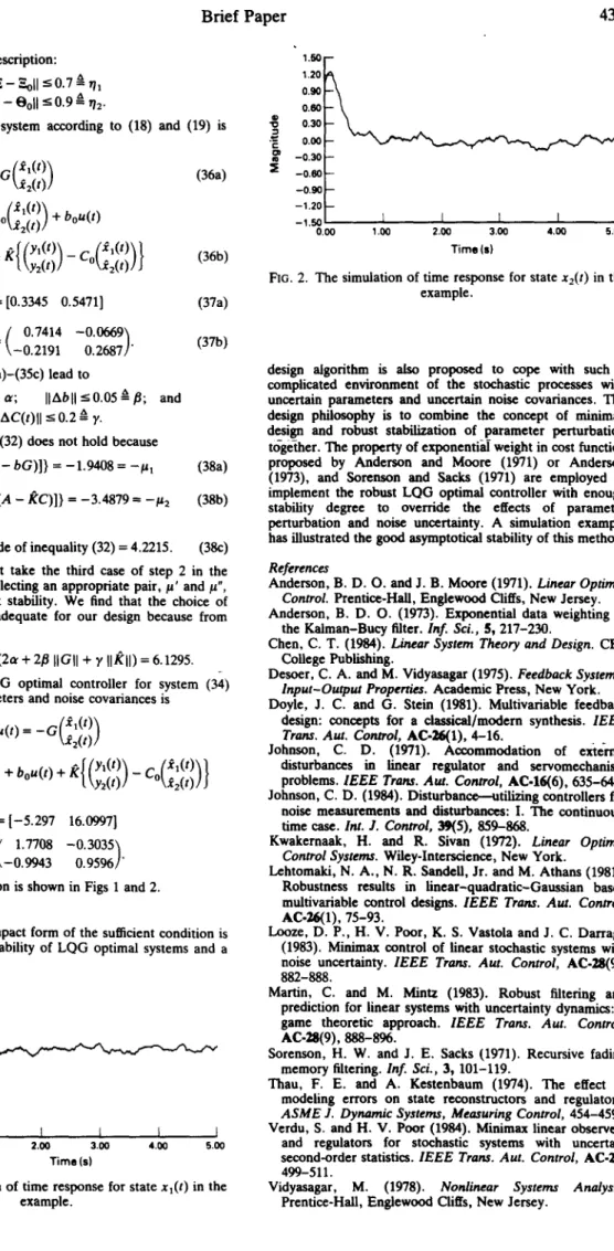
[\y2(t) ] - "~°':~2(t)] J withG = [-5.297 16.0997] / ~ = ( 1.7708-0.3035~ \-0.9943 0.9596]" The result of simulation is shown in Figs 1 and 2.
6. Conclusions
In this paper, a compact form of the sufficient condition is obtained for robust stability of LQG optimal systems and a
1.20 - - 0 . 9 0 ~ 0.60 ~ 0 . 3 0 "~ 0 . 0 0 ~ -0,30 • - 0 . ~ V - 0 . 9 0 - - - 1 . 2 0 0.00 1.00 2.00 3.00 4.00 s.00 T i m e Is)
FIG. 1. The simulation of time response for state
xl(t)
in the example. 1.50 1.20 0.90 0.60 0.30 0.00 - 0 . 3 0 - 0 . 6 0 - 0 . 9 0 - - - 1 . 2 0 - - - 1 . 5 0 0.00 m 1 1 1 I I 't .00 2.00 3.oo 4.oo s.00 T i m e (s)FIG. 2. The simulation of time response for state
x2(t)
in the example.design algorithm is also proposed to cope with such a complicated environment of the stochastic processes with uncertain parameters and uncertain noise covariances. The design philosophy is to combine the concept of minimax design and robust stabilization of parameter perturbation together. The property of exponential weight in cost function proposed by Anderson and Moore (1971) or Anderson (1973), and Sorenson and Sacks (1971) are employed to implement the robust LQG optimal controller with enough stability degree to override the effects of parameter perturbation and noise uncertainty. A simulation example has illustrated the good asymptotical stability of this method.
References
Anderson, B. D. O. and J. B. Moore (1971).
Linear Optimal
Control.
Prentice-Hall, Englewood Cliffs, New Jersey. Anderson, B. D . O. (1973). Exponential data weighting inthe Kalman-Bucy filter.
Inf. Sci., 5,
217-230.Chen, C. T. (1984).
Linear System Theory and Design.
CBS College Publishing.Desoer, C. A. and M. Vidyasagar (1975).
Feedback Systems:
Input-Output Properties.
Academic Press, New York. Doyle, J. C. and G. Stein (1981). Multivariable feedbackdesign: concepts for a classical/modern synthesis.
IEEE
Trans. A ut. Control,
AC-26(1), 4-16.Johnson, C. D. (1971). Accommodation of external disturbances in linear regulator and servomechanism problems.
IEEE Trans. Aut. Control,
AC-I6(6), 635-644. Johnson, C. D. (1984). Disturbance-utilizing controllers fornoise measurements and disturbances: I. The continuous- time
case. Int. J. Control,
39(5), 859-868.Kwakernaak, H. and R. Sivan (1972).
Linear Optimal
Control Systems.
Wiley-Interscience, New York.Lehtomaki, N. A., N. R. SandeU, Jr. and M. Athans (1981). Robustness results in finear-quadratic-Gaussian based multivariable control designs.
IEEE Trans. Aut. Control,
AC-26(1), 75-93.
Looze, D. P,, H. V. Poor, K. S. Vastola and J. C. Darragh (1983). Minimax control of linear stochastic systems with noise uncertainty.
IEEE Trans. Aut. Control,
AC-28(9), 882-888.Martin, C. and M. Mintz (1983). Robust filtering and prediction for linear systems with uncertainty dynamics: a game theoretic approach.
IEEE Trans. Aut. Control,
AC.28(9), 888-896.
Sorenson, H. W . and J. E. Sacks (1971). Recursive fading memory filtering. Inf. Sci., 3, 101-119.
Thau, F. E. and A. Kestenbaum (1974). The effect of modeling errors on state reconstructors and regulators.
A S M E J. Dynamic Systems, Measuring Control, 454-459. Verdu, S. and H. V. Poor (1984). Minimax linear observers
and regulators for stochastic systems with uncertain second-order statistics. I E E E Trans. Aut. Control, AC-28, 499-511.
Vidyasagar, M. (1978). Nonlinear Systems Analysis.
Appendix. Proof o f Theorem 2
From (26), we have
£(t) = * ( t ) / ( 0 ) + * ( t - ~)Zk,4p(r)/(t) d r
£,
+ q~(t - r ) G n ( r ) dr.
When we take the norm operation to both sides of (26), the following inequality is obtained:
Ili(t)ll < II~(t)ll I1,~(0)11
fo' II~(t - r)ll II&~ip(r)~(r)ll d r +
+ I I ~ ( t - r)ll IIGII IIn(t)ll dr. (A1) Since, from (23c)
A- " - - ' " [ & A ( t ) x ( t ) - AB(t)G$(t) \ p(t)x~t) = k&A(t)x(t) - AB(t)GX(t) - KAC(t)x(t)]"
(A2) Consequently from (23), (28) and (A2), we find that
IIZ~p(t)x(t)ll
<-II&A(t)x(t) - AB(t)G$(t)II + II~A(t)x(t) - AB(t)G~(t) - lCAC(t)x(t)ll
<-2 II&A(t)x(t)ll + 2 IIAB(t)G$(t)II
+ IIRII IIAC(t)x(t)ll
--2or IIx(t)ll + 2/3 IIGII II$(t)ll + Y IIKII IIx(t)ll 2a~ II$(t)ll + 2fl IlOll II$(t)ll + ~' II/¢11 II,~(t)ll
= ( 2 ~ + 2fl IIGII + ~' IIKII) II-~(t)ll ( A 3 )
IIGII ~ IIIII + IIIII + IIKII - 2 + IIRII (A4) IIn(t)ll < II~(t)ll + II 0(t)ll
--- ~/(tr (~o + rhI)) + ~/(tr (Oo + r/:I)) (A5) II~(t)lt < m exp ( - ~ t ) (A6) then inequality (A1) becomes
II~(t)ll ~ m I1~(0)11 exp ( - / a ) + m e x p ( - ~ ( t - ~))
x (2e + 2/3 IIGII + r IIKII) II$(r)ll d t Jj m(~/(tr (-So + r/tI)) + X/(tr (Oo + r/:I)) +
x (2 + IIRll) exp (-?~(t - r)) d~. (A7)
Multiplying both sides of (A7) by exp (/at) leads to ]]i(t)]] exp (~t)
f~ (X/(
-< m II•(0)ll + m tr (Et~ + r/tl)) + X/(tr (Oo + r/2I)))(2 + II/(11) exp (~t) d r
£
+ m(2a, + 2/3 Ilall + ~' II/(ll) II~(t)ll exp (/~r) dr = m I1-~(0)11 + (exp (/~t) - 1)((V(tr (-~,, + rhI))
+ V(tr (Oo + 02I)))(2 + IIRIf))/~
+ m(2ac + 2/3 ItG[I + y II/(11) II,~(r)ll exp (~r) dr. By applying the Bellman-Gronwall inequality to the above inequality, we get the following inequality:
II$(t)ll exp(la)<-c(t) + m(2tr + 2fl IIG[I + Y II/(ll)
f2
x e x p ( m ( 2 o l + 2/3 IIGtl
+ ~' II/(ll)(t - s ) ) c ( s ) d s (A8) where
c(t) = m I1~(0)11 + (exp (m) - 1)(k/( tr (Eo + r/¿l)) + X/(tr (Oo + r/2I)))(2 + IIRII)/ta.
Multiplying e x p ( - / a ) to both sides of (A7) and integrating the second term, we obtain the following result:
II$(t)l/- m IIx(0)l[ exp (-/zt)
+ (rn(~/(tr (~.o + 01I)) + V~(tr (Oo + 02I)) x (2 + IIKII)(1 - exp ( - / a ) ) ) / #
+ (/an I1~(0)11 - (V'(tr ( ~ + rhI)) + ~/(tr (Oo + r/zI)))(2 + IIKII))
x (exp ((2mot + 2m/3 llall + m y [I/([I - tot)
- exp ( - / a ) ) / g
+ m(2tr + 2fl IIGII + Y IIKll)(X/(tr ('-o + r/lI))
+ X/(tr (Oo + r/2I)))(2 + II/¢11)(1 - exp (2mtr + 2raft IIa[I + m~, II/~'11 - tot)/
(g(g - m(2~r + 2/3 IIGII + ~' II/¢11))). (A9) S i n c e / ~ > 0 and we assume # > m(2ot + 2/3 IIGll + Y II/(ll). I[$(t)ll in (A9) will converge to a certain value as t----~ oo
(m(X/(tr (-Zo + rhI)) + ~/(tr (Oo + ~/:I)))(2 + Ilgll))/~ + (m(2ol + 2fl IIGll + Y Ilgll)(~/(tr (-% + r/tl)) + X/(tr (Oo + r/:I)))(2 + II/¢11))/
(/~(g - m ( 2 o ~ + 2/3 IIG[I + Y IIKII))) which is dependent on the density of external noises. Hence, the system is asymptotically stable. The proof is completed.