k子棋的複雜度和公平性之探討

國

立

交

通

大

學

資訊科學與工程研究所

碩

士

論

文

k 子 棋 的 複 雜 度 和 公 平 性 之 探 討

On the Complexity and Fairness of the Generalized

k-in-a-row Games

研 究 生：余謝銘

指導教授：蔡錫鈞 教授

k 子棋的複雜度和公平性之探討

On the Complexity and Fairness of the Generalized k-in-a-row Games

研 究 生：余謝銘 Student：Ming Yu-Hsieh

指導教授：蔡錫鈞 Advisor：Shi-Chun Tsai

國 立 交 通 大 學

資 訊 科 學 與 工 程 研 究 所

碩 士 論 文

Submitted to Institute of Computer Science and Engineering College of Computer Science

National Chiao Tung University in partial Fulfillment of the Requirements

for the Degree of Master

in

Computer Science

June 2006

Hsinchu, Taiwan, Republic of China

On the Complexity and Fairness of

the Generalized k-in-a-row Games

Ming Yu-Hsieh

June 23, 2006

Abstract

Recently, Wu and Huang[15] introduced a new game called Connect6, where two players, Black and White, alternately place two stones of their own color, black and white respectively, on an empty Go-like board, except for that Black (the first player) places one stone only for the first move. The one who gets six consecutive (horizontally, vertically or diagonally) stones of his color first wins the game. Unlike Go-Moku, Connect6 appears to be fairer and has been adopted as an official competition event in Computer Olympiad 2006.

Connect(m, n, k, p, q) is a generalized family of k-in-a-row games, where two players place p stones on an m×n board alternatively, except Black places q stones in the first move. The one who first gets his stones k-consecutive in a line (horizontally, vertically or diagonally) wins. Connect6 is simply the game of Connect(m, n, 6, 2, 1). In this paper, we study two interesting issues of Connect(m, n, k, p, q): fairness and complexity. First, we prove that no one has a winning strategy in Connect(m, n, k, p, q) starting from an empty board when k ≥ 4p + 7 and p ≥ q. Second, we prove that, for any fixed constants k, p such that k − p ≥ max{3, p} and a given Connect(m, n, k, p, q) position, it is PSPACE-complete to determine whether the first player has a winning strategy. Consequently, this implies that the Connect6 played on an m × n board (i.e., Connect(m, n, 6, 2, 1)) is PSPACE-complete.

Acknowledgements

I am grateful to my advisor, Dr. Shi-Chun Tsai, for his guidance and en-couragement. I thank my family for their financial and spiritual support.

Table of Contents

1 Introduction and preliminaries 11

2 Fairness 17

3 PSPACE-completeness 23

3.1 Global idea . . . 23

3.2 Construction of winning zone and auxiliary zones . . . 25

3.3 Construction of simulation zone . . . 26

3.3.1 Gadgets for vertices . . . 27

3.3.2 Gadgets for arcs . . . 34

3.4 Put it together . . . 36

3.5 Correctness . . . 39 4 Conclusion and remarks 43 A Drawing 3-planar graphs orthogonally in linear time 45

List of Figures

2.1 Three types of tiles of size (p + 2) × (p + 2), for p = 2. . . 20 2.2 The game board is divided into infinite many 4 × 4 tiles. . . . 20 3.1 The global view of the constructed connect game position. . . 24 3.2 The constructed position in the winning zone. . . 25 3.3 The constructed position in an auxiliary zone. . . 26 3.4 (1a) and (1b) are two kinds of vertices with in-degree and

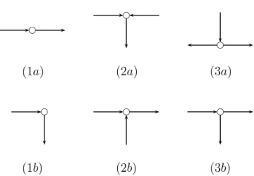
out-degree 1. (2a) and (2b) are two kinds of vertices with in-out-degree 2 and out-degree 1. (3a) and (3b) are two kinds of vertices with in-degree 1 and out-degree 2. The other possibilities can be obtained by flipping or rotating the above. . . 28 3.5 A vertex with in-degree 1 and out-degree 1 corresponds to

Figure 3.4(1a), where node a indicates the entry point and node h the exit point. . . 28 3.6 A vertex with in-degree 1 and out-degree 1 corresponds to

Figure 3.4(1b), where node a indicates the entry point and node h the exit point. . . 29 3.7 A vertex with in-degree 2 and out-degree 1 corresponds to

Figure 3.4(2a), where nodes a and e indicates the entry points and z for the exit point. . . 30 3.8 A vertex with in-degree 2 and out-degree 1 corresponds to

Figure 3.4(2b), where nodes a and e indicates the entry points and z for the exit point. . . 31

10 LIST OF FIGURES 3.9 A vertex with in-degree 1 and out-degree 2 corresponds to

Figure 3.4(3b), where nodes u and z indicate the exit points and a for the entry point. . . 32 3.10 A vertex with in-degree 1 and out-degree 2 corresponds to

Figure 3.4(3b), where nodes u and z indicate the exit points and a for the entry point. . . 33 3.11 (a) A unit component. (b) An arc with 2 unit of length. (c)

Gadget for a bend. . . 35 3.12 A starting vertex with in-degree 1 and out-degree 1

corre-sponds to Figure 3.5. . . 36 3.13 An example with k − p = 4 and the starting vertex gadget

Chapter 1

Introduction and preliminaries

The game family k-in-a-row, or (m, n, k)-Games, is well-known and has been studied for a while. It is a two-player game played on an m × n board. Two players P1 and P2 alternatively place one black and one white stone, respectively, on an unoccupied square on the board and the one who first gets his stones k-consecutive in a line (horizontally, vertically or diagonally) wins. Some of the special (m, n, k)-games, such as TicTacToe ((3, 3, 3)-game) and Go-Moku ((19, 19, 5)-game), are very popular worldwide. Moreover, there are many other modified versions, such as Maker-Breaker version, Inverse version, Periodic version, Higher dimensions version, Multi-Player version and so on[6, 10, 16]. Maker-Breaker is an asymmetric version of the extended (m, n, k)-Game, where in each move, Maker(P1) or Breaker(P2) can place t ≥ 1 stones, and Maker wins by getting his stones k-consecutive in a line, while Breaker wins by preventing Maker from winning. The winning condition of Inverse k-in-a-row game is opposite to that of k-in-a-row game: The one who gets his stones k-in-a-row first loses the game. This version is obviously more complex, since the goal of each player is to avoid his stones k-in-a-row and it is hard to force opponent’s stones row. The board of Periodic k-in-a-row game has some modifications: the left connects with the right, and the top connects with the bottom. It seems fairer with such modification, since all the first moves are equivalent. As for the Higher dimensions version and

12 CHAPTER 1. INTRODUCTION AND PRELIMINARIES Multi-Player version, it just extends the board into three or more dimensions and extend two players to three or more players, respectively. Such modified versions are interesting and generally studied in theoretical computer science and combinatorial game theory.

In this paper, we study a new family of generalized k-in-a-row games: Connect(m, n, k, p, q), which was introduced by Wu and Huang [15]. In Connect(m, n, k, p, q), two players place p stones on an m × n board al-ternatively, except Black places q stones in the first step. The one who first gets his stones k-consecutive in a line (horizontally, vertically or diagonally) wins. For example, TicTacToe is a Connect(3, 3, 3, 1, 1) game, Go-Moku is a Connect(19, 19, 5, 1, 1) game and Connect6 is simply a Connect(∞, ∞, 6, 2, 1) game. For convenience, Connect(∞, ∞, k, p, q) is denoted as Connect(k, p, q)[15]. W.L.O.G., we can assume that max{m, n} ≥ k > p, q > 0. Recently, Connect6 has become an official competition event in the 11th Computer Olympiad in 2006 because of its fairness and state-space complexity. For fur-ther fairness and state-space complexity discussion of Connect6, we refer to Wu and Huang’s paper[15].

Talking about (the generalized) k-in-a-row games, fairness is considered to be the most interesting issue. Herik et al.[14] gave a definition of fairness as follows.

Definition 1 [14] A game is fair if (1) this game has a draw for two perfect players and (2) both players have a roughly equal probability on making a mistake.

However, it is hard to prove that whether both players have a roughly equal probability on making a mistake in general. Wu and Huang[15] gave some empirical results for small cases with k ≤ 9 and k − p ≤ 3. For convenience, this paper focus on the first part of fairness defined above, i.e., for two perfect players, whether Connect(m, n, k, p, q) has a draw or who can win? There are some partial results for this question. For example, the strategy-stealing argument shows that P2 has no winning strategy when

13 q ≥ p : Suppose P2 has a winning strategy, then P1 can make the first move randomly, act as the second player and win by stealing P2’s strategy, which leads to a contradiction. Moreover, for p = q = 1, Herik et al.[14] listed resolved cases for k ≤ 5, while Zetters [17] proved that P2 can tie the game when k ≥ 8 and as a consequence on any finite board. The cases when k = 6, 7 are still unknown. As for the results of the generalized k-in-a-row games, Wu and Huang[15] showed that P1 can win Connect(k, p, q) when p < ⌊_δq2⌋(4δ + 4) + min(q mod δ

2

,⌊8_δ2q⌋), where δ = k − p. Pluh´ar[10]

showed that P2 can tie Connect(k, p, q) when k ≥ p + 80 log2p+ 160 and q = p ≥ 1000, and as a consequence that no one has a winning strategy in Connect(m, n, k, p, q) for any m, n when k ≥ p + 80 log2p+ 160 and p ≥ q. However, this bound can be large even for smaller p. In chapter 2, we give a better result for small p. Indeed, we prove that no one has a winning strategy in Connect(m, n, k, p, q) for any m, n when k ≥ 4p+7 and p ≥ q. As a result, our bound is better than Pluh´ar’s bound for smaller p(≤ 265), although their result is asymptotically better.

Another important issue, for mathematical games, is complexity. The hardness of many popular “small” games is not as easy as we think. Further-more, two-player games are often more complicated than one-player games. For example, it is shown to be PSPACE-complete for Go-moku[11] and Othello[2], EXPTIME-complete for Checkers[12], which is also PSPACE-hard[1], while NP-complete for Minesweeper[4]. For further readings, we refer to Nowakowski’s books[7, 8]. In chapter 3, we study the complexity of Connect(m, n, k, p, q).

Definition 2 [5, 9, 13] A problem is said to be PSPACE-complete if it can be solved within polynomial space and every problem solvable in polyno-mial space can be reduced to it in polynopolyno-mial time. (Note that polynopolyno-mial space/time mentioned here is with respect to the input size.)

Definition 3 For any fixed constants k, p and given an arbitrary Connect(m, n, k, p, q) game position, the decision Connect(m, n, k, p, q) problem is to determine

14 CHAPTER 1. INTRODUCTION AND PRELIMINARIES We will prove that the decision Connect(m, n, k, p, q) problem is PSPACE-complete for k − p ≥ max{3, p} by reducing the generalized geography game played on a planar bipartite graphs of maximum degree 3 to it. The gen-eralized geography game is a two-player game (∃-player and ∀-player) on a directed graph. The ∃-player starts from a specific marked starting vertex, and both players alternatively mark any unmarked vertex to which there is an arc from the last marked vertex. The one who cannot mark vertex any-more loses the game. Sipser[13] showed that the generalized geography game is PSPACE-complete.

Theorem 1 [5, 9, 13] Generalized geography played on a planar bipartite graph of maximum degree 3 is PSPACE-complete.

A key idea of the reduction is to “embed” a graph into the connect game board, and thus two players will be forced to play the geography game in ef-fect. To ensure the embedding can be done in polynomial time, the following theorem is useful.

Theorem 2 [3] There is a linear time algorithm to draw any planar graph of maximum degree 3 on a ⌊V

2⌋ × ⌊ V

2⌋ grid orthogonally, where V is the number of vertices. Moreover, each edge has at most 1 bend.

Once the instance of geography game is drawn orthogonally on a grid, we can transform it into a connect game board efficiently. We will show the details of reduction in chapter 3 and introduce the framework of the algorithm in appendix A. We also need the following definition of threat in a game.

Definition 4 [15] In a Connect(m, n, k, p, q) game, a player is said to have t threats, if and only if his opponent needs to place t stones to prevent him from winning in his next move.

There are other interesting implementation issues, such as game strat-egy, search technique and so on, which are typically addressed in artificial

15 intelligence. Wu and Huang’s paper[15] shows some related results and use-ful references. In this paper, we focus on the theoretical foundation of the games.

Chapter 2

Fairness

Since we have shown that P2 has no winning strategy when q ≥ p, by the strategy-stealing argument, we focus on the cases when q ≤ p in this chapter. The following is our first result.

Theorem 3 No one has a winning strategy in Connect(m, n, k, p, q) for any m, n with max{m, n} ≥ k when q ≤ p and k ≥ 4p + 7.

To prove Theorem 3, we define a new game modified from the Maker-Breaker game, denoted as mMB(n, p) for short, which is a two-player game played on an n × n board. In move 2i − 1, i ∈ N, P1 can choose an integer t, 1 ≤ t ≤ p, and then P1 and P2 are required to place exactly t black stones and t white stones in move 2i − 1 and move 2i, respectively, until there is a winner or no more empty square. If there exist n black stones in a line (horizontally or vertically, but not diagonally), then P1 wins, else P2 wins. Since it can be easily verified that P1 wins when n ≤ p + 1 (trivial case), we can assume n ≥ p + 2. In the following, we will focus on the mMB(n, p) game, and our goal is to prove that P2 has a winning strategy, i.e., preventing P1 from winning. For convenience, we define environment variables ri for the i-th row, 1 ≤ i ≤ n. The value of ri is equal to −1 if there exists a white stone in the i-th row; otherwise, ri indicates the number of black stones in the i-th row. The environment variables cj for the j-th column, 1 ≤ j ≤ n,

18 CHAPTER 2. FAIRNESS are defined similarly, and we let R = {ri|1 ≤ i ≤ n} and C = {ci|1 ≤ i ≤ n}. Moreover, we use (x, y) = B and W to denote that square (x, y) has a black stone and a white stone respectively, and E for empty. We will use a “loop invariant” as shown in Lemma 1 to prove that P1 cannot win, where a “loop” consists of one move of P1 and the countermove of P2.

Lemma 1 In an mMB(p + 2, p) game position, assume there is at most one positive variable in C ∪ R with value 1. Then P2 has a strategy such that, after one move of P1 and one move of P2, (1) P1 cannot win. (2) Before the game terminates, there is at most one positive variable in C ∪ R with value 1.

Proof. Since at most one variable is positive, say ci = 1, there are at most p+ 1 black stones in a line after P1’s move (Note that P1 wins if and only if there are p + 2 black stones in a column or row). We prove the rest by induc-tion on the integer t that P1 chooses. P2’s strategy is given in the induction step below.

Basis: (t = 1) By assumption, there is at most one positive variable ci with value 1. Assume P1 places one black stone at (a, b). First, we consider the case when b 6= i and thus ra ≤ 1, cb ≤ 1, ci ≤ 1, since there may be white stone(s) in row a or column b. If (a, i) = W or (a, i) = E and hence P2 can place a white stone at (a, i), then we have ra ≤ 0, cb ≤ 1, ci ≤ 0 and the lemma holds. Suppose (a, i) = B, then ra ≤ 0 by the assumption that there is at most one positive variable. Hence if there is already one white stone in the i-th column or P2 places a white stone at any empty square in the i-th column, then we are done with at most one variable cb > 0 and cb = 1. The latter case can happen, because P1 has not won yet (that is, the i-th column has an empty square or a white stone in it). Next, we con-sider the case when b = i and then we have ra ≤ 1 and ci ≤ 2. Since there must be an empty square in column i, P2 can place a white stone in the i-th column, and then this lemma holds with at most one positive variable ra= 1.

19 Induction: Assume it is true for all t up to w < p. Consider the case t = w + 1. By the hypothesis, P2 has a strategy Sw using w white stones against the first w black stones P1 placed by ignoring the existence of the (w + 1)-st black stone. Assume P1 placed the (w+1)-st black stone at (a, b). If Sw doesn’t place a white stone at (a, b), then it reduces to the case t = 1. If Sw chooses (a, b), we know that there are at most three variables with positive values (i.e. ra>0, cb >0, ci ≤ 1), and P2 still has two white stones to play (i.e., the one placed at (a, b) is withdrawn). Then P2 can place the two white stones in the a-th row and the b-th column, and we are done with ci ≤ 1. 2

Lemma 2 P2 has a winning strategy in mMB(p + 2, p).

Proof. Since all variables in C ∪ R are zero in the beginning, by Lemma 1, we know that P2 has a winning strategy. 2

Then we have the following obvious consequence. Corollary 1 P2 can win mMB(n, p), when n ≥ p + 2.

Lemma 3 P2 can tie Connect(k, p, q) when q ≤ p and k ≥ 4p + 7. Proof. The strategy for P2 is by divide-and-conquer:

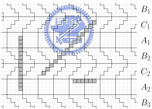
1. Tile the game board with infinite many (p + 2) × (p + 2) tiles as shown in Figure 2.2 (an example of p + 2 = 4). There are three types of tiles: A, B and C as shown in Figure 2.1. Tile B and C are just “twisted” from tile A.

2. In each tile where P1 placed black stones, P2 responds with the same number of white stones in it. This is possible since q ≤ p. If q < p, P2 has extra p − q white stones to play in the following move.

3. Play mMB(p + 2, p) game in each tile, where P2 has enough white stones to play. Note that when playing in a twisted tile P1 tries to

20 CHAPTER 2. FAIRNESS

A

B

C

Figure 2.1: Three types of tiles of size (p + 2) × (p + 2), for p = 2. get (p + 2) black stones horizontally or diagonally. By Lemma 2, we know that P2 has a strategy such that there are at most p + 1 black stones in a line in each tile A(horizontally or vertically), at most p + 1 black stones in a line in each tile B(horizontally or diagonally down), and at most p + 1 black stones in a line in each tile C(horizontally or diagonally up).

B

1

C

1

A

1

B

2

C

2

A

2

B

3

Figure 2.2: The game board is divided into infinite many 4 × 4 tiles. In the whole game board (refer to Figure 2.2), since there are at most (p+1)-consecutive black stones in a vertical line in section {Ai} and at most (p+2)-consecutive black stones in a vertical line in section {Bi,Ci}, we obtain

21 that there are at most (4p+6)-consecutive black stones in a vertical line, i.e., (p+1) in A1, (p+2) in B2, (p+2) in C2, and (p+1) in A2. Similarly, there are also at most (4p+6)-consecutive black stones in a diagonal line (diagonally up and diagonally down). As for the horizontal line, since there are at most (p+1) black stones in section {Ai, Bi, Ci}, there are at most (2p+2)-consecutive black stones in a horizontal line. We show the longest possible black lines with the shaded cells in Figure 2.2. From the above, we get the desired result: there are at most (4p+6)-consecutive black stones in a line (horizontally, vertically and diagonally). 2

Corollary 2 P2 can tie Connect(m, n, k, p, q) for any m, n when q ≤ p and k≥ 4p + 7.

Proof. It is obvious that the strategy for P2 shown in the proof of Lemma 3 can be applied to any finite board. 2

Proof of Theorem 3. This is true since P1 can adopt the strategy for P2, shown in Lemma 3 as well. 2

Chapter 3

PSPACE-completeness

In this chapter, we investigate the computational complexity of the decision

Connect(m, n, k, p, q) problem. We will show that the decision Connect(m, n, k, p, q) problem is PSPACE-complete when k − p ≥ max{3, p}. Recall that the

deci-sion Connect(m, n, k, p, q) problem is to determine whether P1 has a winning strategy when given an arbitrary non-empty Connect(m, n, k, p, q) position, where k and p are fixed constants. Note that this result does not mean to determine which player has a winning strategy when the play starts with an empty board as stated in [5]. Since the given game position in the decision Connect(m, n, k, p, q) problem is not an empty board, q is negligible.

3.1

Global idea

Lemma 4 The decision Connect(m, n, k, p, q) problem is in PSPACE. Proof. Since this game must end in O(mn) steps, this problem can be com-puted by an alternating Turing machince in polynomial time. We know that ATIME(poly) = PSPACE [13]. Hence, this problem is in PSPACE. 2

The next step is to show the PSPACE-hardness of the decision Connect(m, n, k, p, q) problem. It is already known for the case p = 1.

24 CHAPTER 3. PSPACE-COMPLETENESS Lemma 5 [11] The decision Connect(m, n, k, p, q) problem is PSPACE-hard when k ≥ 5 and p = 1.

We focus on the case p ≥ 2 as follows. We show a polynomial time re-duction from the generalized geography game played on a planar bipartite graph of maximum degree 3 to the decision Connect(m, n, k, p, q) problem. For an arbitrary generalized geography game, we will construct a correspond-ing Connect(m, n, k, p, q) game position, where m, n are polynomial in terms of the input size and q is negligible, such that the ∃-player has a winning strategy in the generalized geography game if and only if P1 has a winning strategy from the constructed game position.

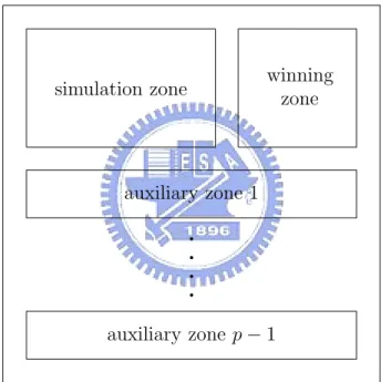
winning zone b b b b simulation zone auxiliary zone 1 auxiliary zone p − 1

Figure 3.1: The global view of the constructed connect game position. The main difference between Go-Moku and Connect(m, n, k, p, q) is that each player can place more than one stone in a move in Connect(m, n, k, p, q) game. In order to deal with this difference, we construct the connect game position with one simulation zone, one winning zone and p − 1 auxiliary zones, as shown in Figure 3.1. The key idea behind the construction is to force each player to place exactly one stone in each of the p − 1 auxiliary

3.2. CONSTRUCTION OF WINNING ZONE AND AUXILIARY ZONES25 zones and the simulation zone until the play in the simulation zone termi-nates, which means no more stone will be placed in the simulation zone. The constructed position in the simulation zone, in effect, forces P1 and P2 to play the generalized geography game. The winner in the simulation zone, can then place stones in the winning zone and will win. Next, we show the constructed position of each zone in details.

3.2

Construction of winning zone and

auxil-iary zones

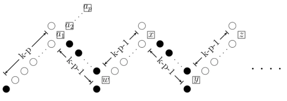
The constructed position in the winning zone is shown in Figure 3.2 and the constructed position in an auxiliary zone is shown in Figure 3.3. Note that the constructed positions of the p − 1 auxiliary zones are the same and the number of the repeated patterns will be determined later. In Figure 3.2 and 3.3, we find that no one has threat in the winning zone (there are only k− p − 1 black and white stones, respectively), and P2 has exactly one threat in each auxiliary zone (the (k − p)-consecutive white stones on the left-hand side), hence p − 1 threats in total, while P1 has no threat in any of the aux-iliary zones yet.

x x xb b b x

a k-p-1

h h hb b b h

k-p-1

26 CHAPTER 3. PSPACE-COMPLETENESS h h h h x a1 a2 b b b ap h b b b k-p x x x b b b w x k-p_-1 h h h b b b h x k- p-1 x x x b b b y x k-p_-1 h h h b b b h z k- p-1 b b b b

Figure 3.3: The constructed position in an auxiliary zone.

3.3

Construction of simulation zone

We construct the simulation zone from an instance of the geography game. The purpose is to force two players to play the generalized geography game in the simulation zone. For a planar bipartite geography graph with maximum degree 3, we will first apply Theorem 2 to draw it orthogonally on a grid, and then construct a corresponding game position in the simulation zone. Next, we give the corresponding constructed positions of the vertices and arcs, which are viewed as gadgets and from which the desired connect position is constructed. Since the vertices and arcs are viewed as gadgets, we can use copies of their mirror images or rotate them 90o_{, 180}o _{or 270}o _whenever necessary .

In the construction, each vertex has one or more entry points and exit points, respectively, and each arc has a head point and a tail point. More specifically, for an arc (u, v), the head point of its corresponding gadget will connect (overlap) the exit point of u’s gadget, and its gadget tail point will connect (overlap) the entry point of v’s gadget. We show the constructions of gadgets as follows.

3.3. CONSTRUCTION OF SIMULATION ZONE 27

3.3.1

Gadgets for vertices

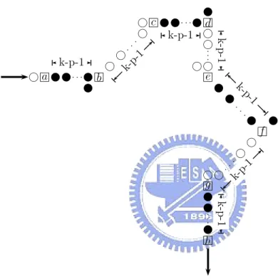
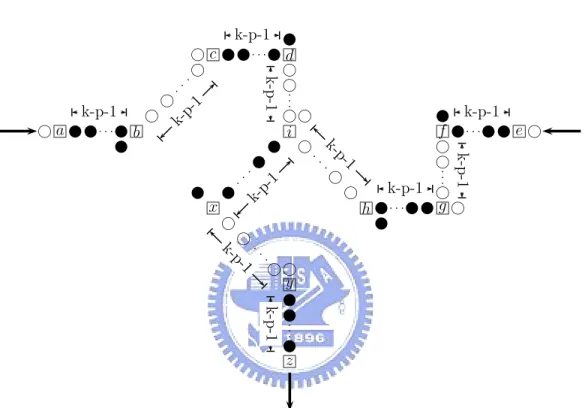
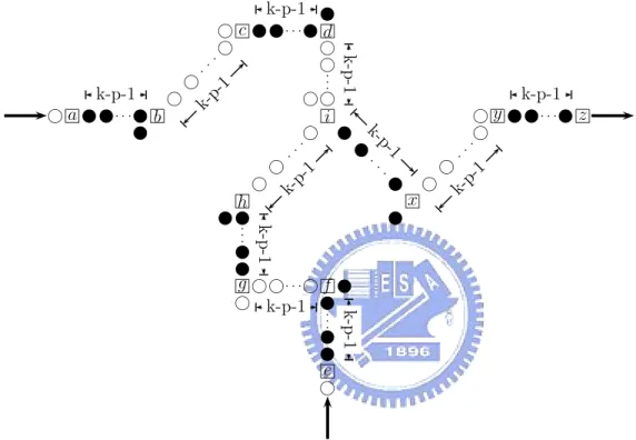
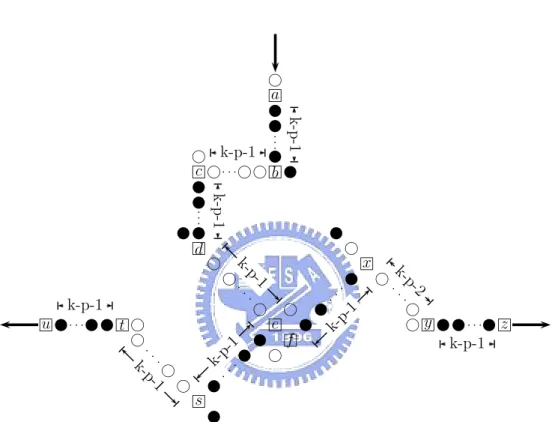
Since the Connect(m, n, k, p, q) game is a two-player game and the general-ized geography game is played on a bipartite graph, we can divide all vertices into two groups, Black and White. Moreover, the starting vertex belongs to Black group, and w.l.o.g., we will illustrate the constructed positions of the vertices in Black group as in the following examples. The constructed po-sitions of the vertices in the White group can be obtained by exchanging the colors. According to [5, 9], there are only three types of vertices in the generalized geography game played on a bipartite graph with maximum de-gree 3, i.e., (1) in-dede-gree 1 and out-dede-gree 1, (2) in-dede-gree 2 and out-dede-gree 1, (3) in-degree 1 and out-degree 2, and for each we construct two kinds of positions as shown in Figure 3.4. The constructed positions of the six kinds of vertices are shown in Figures 3.5 to 3.10. In Figure 3.5 and 3.6, the entry point is at a and the exit point is at h. In Figure 3.7 and 3.8, the two entry points are at a and e, and the exit point is at z. In Figure 3.9 and 3.10, the entry point is at a and the two exit points are at u and z.

28 CHAPTER 3. PSPACE-COMPLETENESS e (1a) e (2a) e (3a) e (1b) e (2b) e (3b)

Figure 3.4: (1a) and (1b) are two kinds of vertices with in-degree and degree 1. (2a) and (2b) are two kinds of vertices with in-degree 2 and degree 1. (3a) and (3b) are two kinds of vertices with in-degree 1 and out-degree 2. The other possibilities can be obtained by flipping or rotating the above. a h x xbbb xb x h h h b b b c h x xbbb x d x h h h b b b e h x x x b b b f x h h h b b b g h x xbbb xh k-p-1 k -p -1 k-p-1 k-p_-1 k- p-1 k-p_-1 k-p-1

Figure 3.5: A vertex with in-degree 1 and out-degree 1 corresponds to Figure 3.4(1a), where node a indicates the entry point and node h the exit point.

3.3. CONSTRUCTION OF SIMULATION ZONE 29 a h x xbbb xb x h h h b b b c h x xbbb x d x h h h b b b e h x x x b b b f x h h h b b b gh x x x b b b h k-p-1 _k-p-1 k-p-1 k -p -1 k-p_-1 k- p-1 k -p -1

Figure 3.6: A vertex with in-degree 1 and out-degree 1 corresponds to Figure 3.4(1b), where node a indicates the entry point and node h the exit point.

30 CHAPTER 3. PSPACE-COMPLETENESS a h x xbbb xb x h h h b b b c h x xbbb xd x h h h b b b i h h h h b b b h xbbb xxg x h h h b b b f h x x xbbb e x h x x x b b b x x h h h b b b yh x x x b b b z k-p-1 k-p-1 k-p-1 k- p-1 k- p-1 k-p-1 k -p -1 k -p -1 k -p -1 k-p_-1 k-p_-1

Figure 3.7: A vertex with in-degree 2 and out-degree 1 corresponds to Figure 3.4(2a), where nodes a and e indicates the entry points and z for the exit point.

3.3. CONSTRUCTION OF SIMULATION ZONE 31 a h x xbbb xb x h h h b b b c h x xbbb x d x h h h b b b i h h h h b b b h x x x x b b b g h h hbbb hf x x x x b b b e h x x x b b b x x h h h b b b y h x xbbb xz k-p-1 k-p-1 k- p-1 k- p-1 k- p-1 k-p-1 k-p-1 k -p -1 k -p -1 k -p -1 k-p_-1

Figure 3.8: A vertex with in-degree 2 and out-degree 1 corresponds to Figure 3.4(2b), where nodes a and e indicates the entry points and z for the exit point.

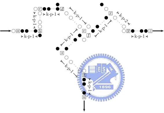
32 CHAPTER 3. PSPACE-COMPLETENESS a h x x x b b b b x h h hbbb c h x x x b b b x d h h h b b b e h x x x b b b s x h h h b b b t h xbbb x x u f h x x x b b b x x h h h b b b y h x xbbb xz k -p -1 k -p -1 k-p-1 k-p-1 k-p-1 k-p_-1 k- p-1 k-p_-1 k- p-1 k-p_-2

Figure 3.9: A vertex with in-degree 1 and out-degree 2 corresponds to Figure 3.4(3b), where nodes u and z indicate the exit points and a for the entry point.

3.3. CONSTRUCTION OF SIMULATION ZONE 33 a h x xbbb xb x h h h b b b c h x xbbb xd x h h h b b b e h f h x x x b b b x h x h h b b b y h xbbb xxz x x x b b b s x h h h b b b t h x x x b b b u k-p_-2 k -p -1 k -p -1 k-p-1 k-p-1 k-p-1 k- p-1 k-p-1 k-p_-1 k-p_-1

Figure 3.10: A vertex with in-degree 1 and out-degree 2 corresponds to Figure 3.4(3b), where nodes u and z indicate the exit points and a for the entry point.

34 CHAPTER 3. PSPACE-COMPLETENESS

3.3.2

Gadgets for arcs

There are two types of arcs: (1) from a vertex in Black group to a vertex in White group, and (2) from White group to Black group. W.L.O.G., we show the construction of type-1 arcs, and type-2 arcs can be obtained by exchanging the colors of the stones. By Theorem 2, we can assume that each arc is horizontal, vertical, or composed of a horizontal segment and a vertical segment. The constructed position of the bend of an arc is shown in Figure 3.11(c). Since the usage of a bend is to connect a vertical segment and a horizontal segment, we can view it as a special vertex with the entry point at a and exit point at i. Furthermore, each straight arc and straight segment may consist of several unit components as shown in Figure 3.11(a), and we define the distance between a and c as a unit for convenience (that is, each unit equals to 2(k − p) in the game board and suppose each side of the cell in the game board has length 1). Thus each arc gadget is of integer unit of length. Moreover, the head point of the arc shown in Figure 3.11(b) is at a and the tail point is at e.

3.3. CONSTRUCTION OF SIMULATION ZONE 35 a h h h x b h b b b k- p-1 x x x b b b c k-p_-1 Length 1

(a)

(b)

(c)

Figure 3.11: (a) A unit component. (b) An arc with 2 unit of length. (c) Gadget for a bend.

36 CHAPTER 3. PSPACE-COMPLETENESS

3.4

Put it together

To obtain the desired connect position in the simulation zone, we need to deal with: (1) the starting vertex and (2) embedding the geography graph into the game board correctly. First the construction of the starting vertex is easy. Since there are only six kinds of vertices, we have six kinds of starting vertices. The constructed position of a starting vertex with in-degree 1 and out-degree 1, as shown in Figure 3.12, is modified from Figure 3.5. The location a is replaced with a black stone and location b with a white stone. The constructed positions of the starting vertex of the other five kinds can be obtained similarly as follows. In Figure 3.6, replace a with a black stone and b with a white stone. In Figure 3.7 and 3.8, replace a, e with black stones and b, f with white stones. In Figure 3.9 and 3.10, replace a with a black stone and b with a white stone. Note that, in the simulation zone, P2 has exactly one threat in the starting vertex (refer to Figure 3.12 for example) while P1 has no threat.

x h x xbbb xh x h h h b b b c1 h c2 b b b cp x xbbb x d x h h h b b b e h x x x b b b f x h h h b b b g h x xbbb xh k-p k -p k-p-1 k-p_-1 k- p-1 k-p_-1 k-p-1

Figure 3.12: A starting vertex with in-degree 1 and out-degree 1 corresponds to Figure 3.5.

Second, we need to embed the geography graph into the game board. By Theorem 2, we can assume the geography graph is drawn orthogonally on a ⌊V

2⌋ × ⌊ V

2⌋ grid, where V is the number of the vertices in the geography graph. Next, we map (i, j) in the grid to (t × L × i + 3 × L, t × L × j + 3 × L) in the game board, where L = 2(k − p) and t is a large enough constant (for

3.4. PUT IT TOGETHER 37 instance, 5 is enough). The reason why we add 3 × L is to reserve spaces for the boundaries.

The constructed position of each vertex has a center point, and we will put the center point at the corresponding coordinate of the vertex. Note that the bend of an arc is viewed as a special vertex. Both of the center points in Figure 3.5,3.6 (Figure 3.7,3.8 and Figure 3.9,3.10) are at e (i and e respectively). The center point of a bend as in Figure 3.11(c) is at e. In Figure 3.5 and 3.6, the distance between the center point and the entry (exit) point has 3

2 units of length. Moreover, the entry (exit) point and the center point is either in the same vertical or horizontal line. The same properties also hold in Figure 3.7 to Figure 3.10 and Figure 3.11(c).

Now we are going to connect the head (tail) point of an arc gadget with the exit (entry respectively) point of the corresponding vertex gadget. Since each arc is of integer units of length, and its corresponding entry point and exit point lie in a line (we can view the bend as a vertex here) with distance a multiple of unit length, we can connect the vertex gadgets and the arc gadgets correctly.

An example with k − p = 4 (ignoring the boundaries) is shown in Figure 3.13. The starting vertex is located at (0,0). The vertices located at {(0,0), (1,1), (0,2)} belong to Black group, and those located at {(0,1), (1,0), (1,2)} belong to White group. The corresponding vertex gadgets in the game board are shadowed with gray color.

38 CHAPTER 3. PSPACE-COMPLETENESS z j z j z j (0,0) (1,0) (0,1) (1,1) (0,2) (1,2) 0 1 0 1 0 1 2 0 1 2 b r b r r r r bb b b r r r r b b bb r r r r bb b b r r rr b b b b rr r r b b b b rr r r b b bb r r r r b b b b r r r r bb b b r r r r b b b b rr r r b b b b rr r r b b b b r r r r b b b b r r r r b b b b r r r r b b b b r r r b rr r r b b b b r r r r r r b bb b r r r r b bb b r r b b b b r r r r b b b b r r rr b b b b r r r r b b b r b b b b r r rr b b b b r r r b b b r rr r b b b b r rr r b r bb b b r r r r bb b b r r r r r r b bb b r r r r b bb b r r b b b b rr r r b b bb r r r r b b b b r r r r b b b b b b r rr r b b b b r rr r b b r r r r b b b b r r r r b b b b r r r r b b b b r r r

Figure 3.13: An example with k − p = 4 and the starting vertex gadget located at (0,0).

3.5. CORRECTNESS 39

3.5

Correctness

We now argue that the constructed position will mimic a generalized geog-raphy game if both of the players play “correctly”. If a player does not play correctly, then it leads to a losing game within a few moves. Let us consider the case that the starting vertex is of in-degree 1 and out-degree 1 as shown in Figure 3.12. The arguments for the other five cases are similar.

Proposition 1 Consider Figure 3.3 and Figure 3.12. In the first move, if P1 does not place stones at one of c1, c2,· · · , cp points in Figure 3.12 and one of a1, a2,· · · , ap in Figure 3.3 in each of the auxiliary zones, then P2 can win immediately.

Proof. Since P1 has no threat, he cannot win in the first move. W.L.O.G., assume that P1 does not place stone at any of a1, a2,· · · , ap in Figure 3.3, then P2can place p white stones at a1, a2,· · · , apand win in the second move. 2

Proposition 2 P1 will have p threats against the second move if and only if he places stones at c1 in Figure 3.12 and a1 in Figure 3.3 in each of the auxiliary zones in the first move. Moreover, P2 has no threat before the second move.

Proof. Clear. 2

Proposition 3 P2 will have p threats against the third move if and only if he places stones at d in Figure 3.12 and w in Figure 3.3 in each of the auxiliary zones in the second move. Moreover, P1 has no threat before the third move. Proof. The same as for Proposition 2. 2

Proposition 4 In the first move, if P1 does not place a black stone at c1 in Figure 3.12 or a1 in Figure 3.3 in one of the auxiliary zones, then P2 can win in two moves.

40 CHAPTER 3. PSPACE-COMPLETENESS Proof. By Proposition 2, P1 will have less than p threats in the second move. W.L.O.G., we can assume that P1 has no threat in the simulation zone (see Figure 3.12). Then by Proposition 3, P2 can place p − 1 stones on w’s in the auxiliary zones to get p − 1 threats and make P1 have no threat. Moreover, P2 can place one white stone at a in the winning zone in Figure 3.2 to get 2 threats. Since P1 has no threat and P2 has more than p threats against the third move, P2 can win in the fourth move. 2

Proposition 5 In the second move, if P2 does not place a white stone at d in Figure 3.12 or w in Figure 3.3 in one of the auxiliary zones, then P1 can win within two moves.

Proof. Similar to Proposition 4. 2

The arguments for the following moves are similar and can be verified easily. Next, we show the cases of different situations.

Proposition 6 The constructed position in Figure 3.9 simulates a vertex of in-degree 1 and out-degree 2 in Black group.

Proof. According to the construction, when entering such a vertex, P1 is forced to place a black stone at a, otherwise, with a similar argument to the proof of Proposition 1, P1 would lose. Then P2 is forced to respond a white stone at b, P1 is forced to respond a black at c, and then P2 is forced to respond a white stone at d. Now, P1 can respond at e or f since p > 1 (if p = 1, P1 is forced to respond at e). Actually, the choice of e and f simulates a vertex with out-degree 2. The arguments for the following moves are straightforward. 2

Proposition 7 The constructed position in Figure 3.10 simulates a vertex of in-degree 1 and out-degree 2 in Black group.

3.5. CORRECTNESS 41 Proposition 8 If a player chooses to visit a visited vertex (not the starting vertex), then it leads to a losing game.

Proof. W.L.O.G., assume P2 revisits a vertex. Then this vertex must be of in-degree 2. Consider Figure 3.7. Assume this vertex has been visited via the left entry point and hence there must be black stones at a, c and i, and white stones at b and d, otherwise P1 would have lost the game earlier. Next, according to the construction of the connect position, when reentering such a vertex, P1 is forced to place one black stone at e, P2 is forced to respond a white stone at f , and P1 is forced to respond a black stone at g. Now, in the whole game board, P2 has no threat and P1 has p threats by Proposition 2. In the auxiliary zones, P2 can get p − 1 threats in the following move and make P1 no threat there. However, in the simulation zone (Figure 3.7), P2 can only make P1 no threat but cannot create new threat at the same time, since there is already a black stone at i. Finally, similar to the argument in Proposition 4, P2 will lose in two moves and P1 will win. The case of Figure 3.8 is similar. 2

Proposition 9 If P2 chooses to visit the starting vertex, then he will lose. Proof. Similar to Proposition 8. 2

Since the play in the simulation zone will terminate when a player chooses to revisit a vertex and the opponent will then win, we have shown that the ∃-player has a winning strategy in the generalized geography game if and only if P1 has a winning strategy from the constructed position of the Connect(m, n, k, p, q) game. Moreover, the setting k − p ≥ p and the large enough constant distance between any two mapped coordinates ensure the required empty squares, e.g. c1, c2,· · · , cp in Figure 3.12, will not be affected by any components of the constructed position. The reason why k − p ≥ 3 is trivial, i.e., in Figure 3.7, there are two consecutive black stones next to b, and hence k − p must be greater than 2.

42 CHAPTER 3. PSPACE-COMPLETENESS Finally, we have to make sure that the reduction can be done in polyno-mial time. We estimate the required size for each zone of the constructed position in the following:

1. Winning zone: O(k − p) × O(k − p), see Figure 3.2.

2. Simulation zone: Since k and p are fixed constants, the size of the simulation zone is bounded by O(V ) × O(V ), refer to Theorem 2. 3. Auxiliary zone: We now determine the number of the repeated parts

in Figure 3.3. Since we require that the play in the simulation zone always terminates a few moves earlier than the play in the auxiliary zones, the number of the repeated parts is related to the size of the simulation zone. Hence, the required size is O(1) × O(V ).

Therefore, we obtain that m = O(V ) and n = O(V ). Since the construction mentioned above can be done in polynomial time, we have the following lemma.

Lemma 6 The decision Connect(m, n, k, p, q) problem is PSPACE-hard when k− p ≥ max{3, p} and p ≥ 2.

Theorem 4 The decision Connect(m, n, k, p, q) problem is PSPACE-complete when k − p ≥ max{3, p} and p ≥ 2.

Proof. Immediately from Lemma 4 and 6. 2

Corollary 3 To determine whether P1 has a winning strategy in a given non-empty Connect6 game position is PSPACE-complete.

Proof. Immediately from Theorem 4. 2

Corollary 4 The decision Connect(m, n, k, p, q) problem is PSPACE-complete when k − p ≥ max{3, p}.

Chapter 4

Conclusion and remarks

The main results in this paper are: (1) Fairness issue: no one can win Connect(m, n, k, p, q) for any m, n when q ≤ p and k ≥ 4p + 7. (2) Complex-ity issue: The decision Connect(m, n, k, p, q) problem is PSPACE-complete when k − p ≥ max{3, p}.

Open problems: (1) Can we have a better bound than the first result, since Zetters[17] showed that P2 can tie the game when k ≥ 8 and p = q = 1? (2) Is the decision Connect(m, n, k, p, q) problem still PSPACE-complete if the restriction, k − p ≥ max{3, p}, is removed?

Appendix A

Drawing 3-planar graphs

orthogonally in linear time

We introduce the framework of a linear time algorithm for drawing 3-planar graphs orthogonally (refer to Theorem 2), which is proposed by Kant[3] and used in our reduction in chapter 3. For details, we refer to Kant’s paper[3].

Input: A 3-planar graph of n vertices.

(1) Find vertices v1, v2, vn such that v2 and vn are v1’s neighbors. This can be done in O(n) time easily.

(2) Given v1, v2 and vn, there is a O(n) time algorithm to sort the vertices in a special order: {v1, v2,· · · , vn}, which is called lmc-ordering. (3.1) For any triconnected 3-planar graph, there is a O(n) time algorithm to

draw it on a grid orthogonally according to the lmc-ordering.

(3.2) For any biconnected 3-planar graph, we can decompose it into tricon-nected components in O(n) time. Calling (3.1) as subroutines, there is a O(n) time algorithm to draw it on a grid orthogonally.

(3.3) For an arbitrary 3-planar graph, we can decompose it into biconnected components in O(n) time. Calling (3.2) as subroutines, there is a O(n) time algorithm to draw it on a grid orthogonally.

Bibliography

[1] A.S. Fraenkel, M.R. Garey and D.S. Johnson, The Complecity of Check-ers on an N × N Board - Preliminary Report, In the 19th IEEE Sympo-sium on Foundations of Computer Science, 55-64, 1978.

[2] S. Iwata and T. Kasai, The Othello game on an n×n board is PSPACE-complete, Theoretical Computer Science, 123: 329-340, 1994.

[3] G. Kant, Drawing planar graphs using the canonical ordering, Algorith-mica, 16(1): 4-32, 1996.

[4] R. Kaye, Minesweeper is NP-complete, Mathematical Intelligencer, 22(2): 9-15, 2000.

[5] D. Lichtenstein and M. Sipser, Go is polynomial-space hard, Journal of the ACM, 27: 393-401, 1980.

[6] W.-J. Ma, Generalized Tic-tac-toe, http://www.klab.caltech.edu/ ~ma/tictactoe.html, 2005.

[7] R.J. Nowakowski, Games of no chance: combinatorial games at MSRI, Cambridge University Press, 1994.

[8] R.J. Nowakowski, More games of no chance, Cambridge University Press, 2002.

[9] C.H. Papadimitriou, Computational complexity, Addison Wesley Pub-lishing Company, 1994.

48 BIBLIOGRAPHY [10] A. Pluh´ar, The accelerated k-in-a-row game, Theoretical Computer

Sci-ence, 270: 865-875, 2002.

[11] S. Reisch, Gobang ist vollst¨andig (Gobang is PSPACE-complete), Acta Informatica, 13: 59-66, 1980.

[12] J.M. Robson, N by N Checkers is EXPTIME complete, SIAM Journal on Computing, 13(2): 252-267, May 1984.

[13] M. Sipser, Introduction to the Theory of Computation, PWS Publishing Company, 1997.

[14] H.J. van den Herik, J.W.H.M. Uiterwijk and J. van Rijswijck, Games Solved: Now and in the Future, Artificial Intelligence, 134: 277-311, 2002.

[15] I.-C. Wu and D.-Y. Huang, A new family of k-in-a-row games, In the 11th Advances in Computer Games Conference (ACG’11), Taipei, Taiwan, September 2005.

[16] J. Yolkowski, Tic-tac-toe, http://www.stormloader.com/ajy/ tictactoe.html, 2003.

[17] T.G.L. Zetters, 8(or More) in a Row, American Mathematical Monthly, 87: 575-576, 1980.