A Theory for Multifilamentary Pattern Formation in Semiconductors
Fu-Sin Lee and Yi-Chen Cheng
Department of Physics, National Taiwan University, Taipei, Taiwan 106, R.O.C.
(Received November 24, 1999)
A theory for multifilamentary pattern formation in semiconductors with an S-shaped neg-ative conductivity (SNDC) is presented. The theory is based on the basic equations in elec-trodynamics and the impact ionization mechanism with double impurity trap levels, which is widely accepted as the mechanism for SNDC. No extra physical quantities and/or parameters are introduced in the theory. The steady-state of the dynamical equations is a one-dimensional reaction-diffusion type equation, which provides stable multifilamentary pattern structures. The stability analysis for the steady-state N-filament (N=2, 3, and 4) solution is given. PACS. 72.20.Ht – High-field and nonlinear effects.
PACS. 47.54.+r – Pattern selection; pattern formation.
PACS. 72.20.–i – Conductivity phenomena in semiconductors and insulators.
I. Introduction
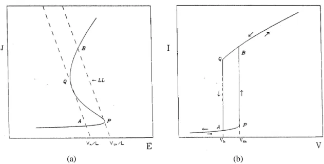
It is well known that a semiconductor with an S-shaped current-density-field (J-E)
char-acteristic (Fig. 1(a)) will exhibit a hysteresis loop in the current-voltage (I-V ) curve (Fig. 1(b)),
when the system is connected in series with a dc bias voltageV and a light load resistance R. The
slope of the load line (LL in Fig. 1(a)) does not change if the load resistanceR is a constant, but
the position of the horizontal (vertical) intercept varies as the applied field (i.e., the bias voltage) varies. The holding voltage Vh and the threshold voltage Vth are, respectively, the bias voltage for which the load line passes through point Q or P in Fig. 1(a); in between P and Q the load line intercepts theJ-E curve in three points. Outside P and Q, the load line intercepts the J-E curve
in only one point. The J-E curve from P to Q has a negative differential conductivity (NDC) dJ=dE < 0, and the system is unstable when it is operating in the regime of NDC [1]. The
system is therefore in a bistable state in the portion of AP or QB of the J-E curve, where the J-E curve intersects the load line three times, but only two of them are stable. The corresponding I-V curve (Fig. 1(b)) reflects the bistable nature which results in a hysteresis loop. When the
bias voltage increases slowly from a low voltage and reaches the threshold voltageVth , the system will jump abruptly from the low-current-density state P to the high-current-density state B (not along the path P to Q). In the reverse direction of decreasing the bias voltage slowly, the current changes gradually atVth , but when the voltage reachesVh the system will drop abruptly from the high-current-density state Q to the low-current-density state A, thus forming a hysteresis loop.
155 ° 2000 THE PHYSICAL SOCIETYc OF THE REPUBLIC OF CHINA
(a) (b)
FIG. 1. (a)J -E characteristic for an SNDC semiconductor; and (b) the corresponding I-V curve.
FIG. 2. MeasuredI-V curve for low-temperature n-GaAs, reported by Mayer et al. in Ref. 2. The graph
is reproduced from Ref. 2.
However the above picture is valid only when the system is always in a homogeneous steady state. In some systems the hysteresis loop may have more complicated structures if spatially inhomogeneous structures develop. For example, in low temperature n-GaAs [2] the measured
hysteresis I-V curve has a more complicated shape as shown in Fig. 2. The zigzag (consecutive
filament. Two-dimensional images of current filaments are observed by using low temperture electron-scanning micoscopy [2].
Theoretical explanation of the above multifilament observation is, so far, not satisfactory. One of the popular model is the one-dimensional reaction-diffusion (RD) equation known as the Schl¨ogl-type model [3], which has steady-state multifilamentary solutions. But it is known that these steady-state solutions are unstable [4], thus it is not a satisfactory model. To the authors’ knowledge, there have been two theories which tried to resolve the problem of stability of current filaments in bistable semiconductor systems [5, 6]. Both theories used the one-dimensional RD equation we have just mentioned, but with an additional constrain to the equation. Kardell et
al. [5] introduced an additional variable to the RD equation, and thus becomes a two-variable
model which can have stable multifilamentary solutions. But this model requires non-negligible hoppings (or tunnelings) of electrons between neighboring impurity sites, which seems not to be a practical assumption for an impurity concentration around 1015/cm3. Recently Alekseev et al. [6] studied the RD equation with global coupling by external circuit. They found that in the strong coupling (large load resistance R) case the unstable mode may be stablized. But in the
weak coupling (small R) or no coupling (R = 0) case, all stationary nonuniform solutions are
still unstable. Therefore their theory can not explain the experimental result of Mayer et al. [2] which was performed in the weak coupling (small R) limit.
In this paper we propose a simple and realistic model which can support stable steady-state mutifilamentary solutions in weak and no coupling (R = 0) limit. The theory is based on
the basic equations in electrodynamics and the widely accepted two-trap-level model for SNDC materials with no extra assumptions. Electrons trapped in the impurity sites can gain or lose energy to change their energy level (ground, or first-excited, or the conduction level), but they can not hop from one site to another. Our model has steady-state multifilamentary solutions which are proven to be stable. In the steady state, our model is the same as the RD equation. But in the time-dependent case (as unstable modes must be time-dependent) our model introduces an additional spatial dependent differential equation to couple the RD equation. Thus it imposes an additional constraint on the RD equation which is an important factor to stablize the unstable steady-state multifilamentary solutions as previous theories suggested [5, 6]. It is worthwhile to point out that the constraint comes naturally from the basic equations of electrodynamics and we do not introduce it to our model artificially. For completeness, we do stability analysis for the steady-state solutions of our model at the end of the paper. The result confirms that our solutions are stable.
II. The model
A simple two-level model (the ground state and the first excited state of the impurity) is adequate to explain the origin of an S-shaped NDC [7, 8]. In this model there are three energy levels for an electron: the ground state and the first excited state of the donor impurities, in addition to the conduction level. We adapt this model in the following analysis. The electron densities in these three levels are governed by the generation-recombination (g-r) processes which give rise to the rate equations for the electron densities:
dn
dn0
dt = g2(n; n0; n1; E); (2)
dn1
dt =¡ g1(n; n0; n1; E)¡ g2(n; n0; n1; E); (3)
where n, n0, and n1 are, respectively, the electron density of the conduction band, the ground state and the first excited state of the donors. The functions g1 andg2 are rate functions in the g-r processes and can be written as [7]
g1 = X1sn1¡ T1s(ND¡ n0¡ n1)n + X1¤(E)n1n + X1(E)n0n; (4)
g2 =¡ X¤n0+ T¤n1¡ X1(E)n0n; (5)
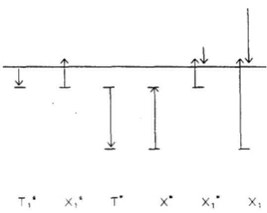
whereND is the effective total donor concentration. The physical meaning of the rate coefficients Xs
1, T1s etc. are shown in Fig. 3. Among these rate coefficients, X1 and X1¤ are electric field dependent [7] which can be written as (Shockley lucky electron model) [9, 10]
X1(E) = C0e¡ "0=(e`E); (6)
X1¤(E) = C1e¡ "1=(e`E); (7)
whereC0 andC1 are constants,` is the electron mean free path, and "0 and"1 are, respectively, the binding energy of the ground state and the first excited state of the donor impurity. In the homogeneous steady stateg1 = g2 = 0, the condition of charge neutrality ½(n; E) = eND¡ e(n+ n0 + n1) = 0 will result in a multi-valued conduction electron density n = n(E) in a certain range of the electric field E, which in turn produces an S-shaped J-E characteristic.
Now we construct the model which is able to describe the formation of multiple current filaments in semiconductors with an S-shaped NDC. All our starting equations are basic equations in electrodynamics:
@n @t ¡
1
er ¢J = g1(n; n0; n1; E); (8)
J = en¹E + eDrn; (9)
²r ¢E = ½(r; E) ´ eND¡ e[n(r; t) + n0(r; t) + n1(r; t)]; (10)
r £ H = ²@E@t + J´ J0: (11)
Equation (8) is the equation of continuity (conservation of charge), where J is the conduction
current density. J is the sum of the drift and the diffusion current densities (cf. Eq. (9)), where ¹ and D are the electron mobility and the diffusion constant, respectively. Equation (10) is the
Gauss’s law and Eq. (11) is the Ampere’s law that the total current density J0 consists of the conduction and the displacement current densities, with ² the dielectric constant of the sample.
We consider a rectangular sample in the region ¡ Lx · x · Lx, ¡ Ly · y · Ly, and ¡ Lz · z · Lz. An external dc bias voltage V is applied in the z-direction, which is connected in series with a light load resistant R such that the system will be operating in the
bistable state for a certain range of V (cf. Fig. 1(a)). To study filament formation we have to
consider the conduction electron density n and the electric field E to be dependent on r. It is
a good approximation that there is no spatial z-dependence and we may write n = n(x; t) and
E = Ex(x; t)^x + Ez(t)^z, if we consider the case Ly ¿ Lx thus y-dependence can be neglected. As in many applications [7], we consider the case that the relaxation of the g-r processes is much faster than the dielectric relaxation, and we can approximateg1¼ 0 and g2¼ 0. This is equivalent to say that the S-shaped J-E characteristic is an intrinsic property of the sample. The charge
density½ = ½(n; E) = eND¡ e(n + n0+ n1) can then be obtained by eliminating n0 andn1 via Eqs. (2) and (3). The dynamical equatuins become
@n @t = @ @x µ n¹ Ex+ D@n @x ¶ ; (12) ²@ @xEx= ½(n; E); (13) ²@Ez @t = V AR¡ µ L z AR + e¹ 2Lx Z Lx ¡ Lx ndx ¶ Ez; (14)
where A = 4LxLy is the cross sectional area of the sample. Because Ex is an induced field and we expect that jExj ¿ jEzj, therefore ½(n; E) ¼ ½(n; Ez). The variable Ex can then be eliminated by Eq. (13), and we obtain the following dynamical equations:
@u @t = D @2u @x2 + ¹f (u; Ez) + @u @x µ ¹ Z x ¡ Lx f(u; Ez)dx0+ D@u @x ¶ (15) @Ez @t = V ²AR ¡ µ L z ²AR+ e¹ 2²Lx Z Lx ¡ Lx eudx ¶ Ez; (16)
TABLE I. Typical material parameter values corresponding to n-GaAs at 4:2±K for the two-level generation-recombination mechanism [7]. parameter value Ts 1 10¡ 6 cm¡ 3 s¡ 1 T¤ 106s¡ 1 X¤ 104s¡ 1 Xs 1 2£ 107 s¡ 1 X1 5£ 10¡ 8exp(¡ 6=E) cm3 s¡ 1 X1¤ 10¡ 6exp(¡ 1:5=E) cm3 s¡ 1 ND 1015 cm¡ 3 ¹ 104 cm2 V¡ 1s¡ 1 ² 8:85£ 10¡ 13 F cm¡ 1 Lx 1:5£ 10¡ 2 cm
where we have defined u ´ ln n and f(u; Ez) ´ ½(eu; Ez)=². The parameter values used in obtaining½(n; Ez) are tabulated in Table I.
III. Steady state solutions
We are looking for the steady-state solutions of Eqs. (15) and (16). We consider the extreme light load limiting case that R ! 0, as most of the experimental observations of the
mutifilamentary pattern were done in this limit. Equation (16) then tells us that @Ez=@t = 0 and Ez = V =Lz is a constant for a dc bias V . Thus we may consider Ez is the control parameter in Eq. (15). Note that the quantity in the parentheses of the right hand side of Eq. (15) is zero in the steady state. This can be understood as follows. The quantity is proportional toJx which is the x-component of the conduction current density (cf. Eq. (9)). Because the circuit is open in
the x-direction, Jx = 0 at the boundaries x =§ Lx for allt. In the steady state @n=@t = 0, and therefore @Jx=@x = 0 by Eq. (8) (g1=0). Thus Jx= 0 everywhere.
The equation we have to solve in the steady state is therefore the following:
D@
2u
@x2 + ¹f(u; Ez) = 0: (17)
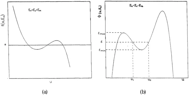
In this equationEz is considered as a control parameter. Before solving this equation, it is helpful to study the functional behavior off(u; Ez) vs. u for a given Ez. We find that the characteristic of the function f(u; Ez) vs. u depends on the value of Ez. In Fig. 4(a) we show that when Eh < Ez < Eth f (u) = 0 has three roots, where Eh (Eth ) is the electric field corresponding to the bias voltage Vh (Vth ) shown in Fig. 1(b). In other range of Ez, f(u) = 0 has only one root.
Therefore if we define a function Á(u; Ez) as (u0 is an arbitrary value ofu)
Á(u; Ez) = ¹ Z u
u0
f(u0; Ez)du0; (18)
then the characteristic of Á(u; Ez) vs. u has the form as shown in Fig. 4(b). It is important to note that the function Á(u; Ez) vs. u has a local minimun when the electric field Ez is in the rangeEh < Ez < Eth , i.e., it looks like a potential well. WhenÁ(u) has the shape of a potential well, Eq. (17) can be solved in a rather easy way [11]. Because the formation of current filaments occurs only in the field range Eh < Ez < Eth , it is sufficient for us to consider the case that
Á(u) has a local minimun.
Equation (17) can be written as [11] 1 2D µ du dx ¶2 + Á(u; Ez) = "; (19)
where " is an integrating constant. To solve Eq. (19), we may interpret this equation in terms of
the terminology in mechanics. If we imaginex as “time”; D, u, and Á, respectively, as the “mass”,
“displacement”, and “potential energy” of the system, then" plays the role of the “total energy”.
From Fig. 4(b), we see that when" lies in a certain range "m in (Ez) < " < "m ax (Ez), then there is a bounded solution in which the “motion” of u is confined in the region of the potential well
(u1(Ez)· u · u2(Ez)). This is the solution we are looking for. In this solution u (and
(a) (b)
FIG. 4. Plot of the functionf (u; Ez) vs. u (a), and the function Á(u; Ez) vs. u (b), for Ezin the range
therefore the electron density n) varies with x and thus current filaments are formed. Note that
for u outside the potential well, the only possible solution is " = Á(u) which implies du=dx = 0,
i.e., a homogeneous state. Otherwise the “motion” of u will be unbounded, which is unphysical
because in a system the electron density should be positive and finite with values within a certain region only. Therefore it is sufficient for us to consider the case that "m in (Ez) < " < "m ax (Ez). In this range of ", Eq. (19) can be numerically solved to give
x(u) =§pD=2 Z u u1 du p "¡ Á(u; Ez) ; (20)
where the upper limit of the integration u· u2.
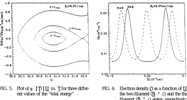
However it is more instructive to solve Eq. (19) in the following way. We note that if
"m in < " < "m ax , then the graph du=dx vs. u is a closed curve for u1 · u · u2, as shown in Fig. 5. It is reasonable to use the periodic boundary condition for u(x) (with period 2Lx), thus u(¡ Lx) = u(Lx) and du=dx(¡ Lx) = du=dx(Lx). Then we start from x = ¡ Lx, which corresponds to some point in Fig. 5, and increase x until x = Lx. The corresponding point (for eachx) in Fig. 5 will move along the closed curve du=dx vs. u, and returns to the starting point
when x = Lx, because u(Lx) = u(¡ Lx) and also du=dx(Lx) = du=dx(¡ Lx). However it is possible that the corresponding point in Fig. 5 moves around the closed curve N times when x
increases fromx =¡ Lx tox = Lx, whereN is some integer. Therefore we have a “quantization rule” as in the old theory of quantum mechanics:
2Lx
N = D
I dq
p ; (21)
where the “coordinate”q is u and the “momentum” p is D(du=dx). The integral is over one period
in the q-space. There are N periods as x increases from¡ Lx toLx. The explicit expression for Eq. (21) is Lx N = r D 2 Z u2(";Ez) u1(";Ez) du p "¡ Á(u; Ez) : (22)
This equation implicitly suggests that the “energy” " depends on the number of period N , which
may be denoted as "N. Thus when the number of period increases from N to N + 1, the corresponding “energy” goes from"N to"N+1, i.e.," is quantized as in the old theory of quantum mechanics. We note that"N is a function ofEzand denote it as"N(Ez). With the aid of Eq. (22), the electron densityn as a function of x is plotted in Fig. 6 for the cases of N = 2 and 3.
The physical significance of the “quantization rule” imposed by Eq. (21) can be understood as follows. For a given bias voltageV (then the field Ez = V =Lz), there are only several integers Ni (sayi = 1; 2;¢¢¢; p) which satisfy Eq. (21). This means that for this V the system can only sustain Ni-filament state (i = 1; 2;¢¢¢; p). The conditions that Ni-filament may exit for a given V , will affect the structure of the hysteresis loop in the I-V curve of the system. This is the topic
FIG. 5. Plot ofD(du=dx) vs. u for three
differ-ent values of the “total energy” ".
FIG. 6. Electron densityn as a function of x for
the two-filament (N = 2) and the
three-filament (N = 3) states, respectively.
IV. Stepped hysteresis loop
In this Section we describe how the small steps in the hysteresis loop can be formed. We denote the integrated value of the integral in the right hand side of Eq. (22) asS("; Ez):
S("; Ez) = r D 2 Z u2(";Ez) u1(";Ez) du p "¡ Á(u; Ez) : (23)
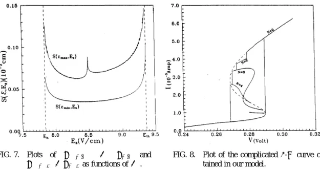
In this equation " is a continuous (not quantized) parameter which is restricted in the range "m in (Ez)· " · "m ax (Ez). It can be shown that for a given Ez, S("; Ez) has a minimun value Sm in (Ez) when " = "m in (Ez), and a maximun value Sm ax (Ez) when " = "m ax (Ez). From the quantization rule of Eq. (21) (where " = "N(Ez)), we have
Sm in (Ez)· Lx
N · Sm ax (Ez): (24)
This inequality tells us that for a given Ez, there may exist one or several N which satisfy the condition (24). The number N, which satisfies the condition (24), is the number of filaments in
the sample. The steady-state N-filament solution is denoted as u(N)(x), where N must satisfy the inequality (24). In order to obtain the stepped hysteresis loop, we have to know the allowed
N as a function of Ez. We plot the Ez-dependence of Sm in and Sm ax in Fig. 7. From Fig. 7 the allowedN can be obtained for a given Ez by using inequality (24). TheI-V hysteresis loop is plotted in Fig. 8, which contains several small steps. Figure 8 is qualitatively similar to the experimental results of Mayer et al. [2].
FIG. 7. Plots of S("m in ) ´ Sm in and
S("m ax)´ Sm ax as functions ofEz.
FIG. 8. Plot of the complicated I-V curve
ob-tained in our model.
V. Stability analysis
Stability is an important question for theoretical models which have steady state multifil-amentary solutions as we have pointed out in Introduction. The Schl¨ogl-type reaction-diffusion (RD) equation [3] is
@u @t = D
@2u
@x2 + f(u; ® ); (25)
where the nullcline of f(u; ® ) = 0 is N-shaped (® is the control parameter). With the Neumann
boundary conditions, @u(x; t) @x ¯ ¯¯ ¯ x=Lx = @u(x; t) @x ¯ ¯¯ ¯ x=¡ Lx = 0;
Eq. (25) is known to have steady-state multifilamentary solutions. However these solutions are unstable against small time-dependent fluctuations [4], therefore it is not a satisfactory model. Although the steady-state equation for our model Eq. (17) is quite similar to the Schl¨ogl model, the time-dependent equation for our model (Eq. (15) is different from the Schl¨ogl model Eq. (25) as it introduces an additional constraint to the RD equation. Equation (15) is an integro-differential equation which comes from two differential equations, Eqs. (12) and (13). Therefore our model has an extra spatial-dependent differential equation for Ex, which is the additional constraint we find in our model. It is worthwhile to point out that the constraint comes naturally from basic equations of electrodynamics and we do not introduce it to our model artficially. The additional constraint will affects the stability of the multifilamentary solutions as suggested in previous studies [5, 6]. It turns out that the steady-state multifilamentary solutions of our model are stable, which we will show in the followings.
Without loss of generality, we consider the extreme light load limit R ! 0 as we have
done in Sec. III. In this limit Ez = V=Lz by Eq. (16), andEz can be considered as the control parameter, which is kept as a constant in the following analysis. We think it is more convenient to consider the dynamical equations forn than those for u (u = ln n). The time-dependent equations
of our model are Eqs. (12) and (13),
@n @t = @ @x µ n¹ Ex+ D@n @x ¶ ; ²@ @xEx= ½(n; E):
We expand the variables n, Ex; and½ in terms of the Fourier components, n(x; t) =X l nl(t)ei l¼ Lxx; (26) Ex(x; t) = X l Ex;l(t)ei l¼ Lxx; (27) ½(n; Ez) = X l ½l(t)ei l¼ Lxx: (28)
Equations (12) and (13) become
@nl @t =¡ µ l¼ Lx ¶2 Dnl+ i¹0l¼ Lx X l0 nl0Ex;l¡ l0; (29) and i²l¼ LxEx;l = ½l: (30) By eliminating Ex;l, we get @nl @t =¡ µ l¼ Lx ¶2 Dnl+ ¹0l ² X l06=l nl0½l¡ l0 l¡ l0: (31)
Because we are considering the stability of the steady-state solution with N -filament, we may
decompose the components nl and ½l into time-independent and time-dependent parts. Suppose n(x; t) is very close to the steady-state N -filament solution nN(x)´ exp[u(N)(x)], we may write
n(x; t) = n(N)(x) + ±n(N)(x; t); (32)
where ±n(N )(x; t) and ±½(N )(x; t) denote small time-dependent fluctuations; and ½(N)(x) ´
½(n(N )(x); E
z): The time-independnet parts n(N)(x) and ½(N )(x) are, respectively, expanded in terms of the Fourier components:
n(N)(x) =X l n(N )l eiLxl¼ x; (34) ½(N )(x) =X l ½(N)l eiLxl¼ x: (35)
Similarly the time-dependent parts ±n(N )(x; t) and ±½(N )(x; t) can be expanded as
±n(N)(x; t) =X l ±n(N)l (t)eiLxl¼ x; (36) ±½(N)(n) =X l ±½(N)l (t)eiLxl¼ x=X l X l0 ½0l(N )¡ l0±n(N )l0 (t)ei l¼ Lxx; (37)
where½0l(N) is the Fourier component of@½(n(N ); E
z)=@n(N ): @½(n(N); Ez) @n(N) = X l ½0l(N )eiLxl¼ x: (38)
From these expansions, we see thatnl(t) = n(N)l + ±n(N)l (t) and ½l(t) = ½(N)l + ±½(N)l (t). We can then linearize Eq. (31) (by using Eq. (37)) and neglect higher order terms of ±n(N)l (t) to obtain @±n(N )l @t = 1 X l0=¡ 1 Mll(N)0 ±n(N )l0 ; (39) where Mll(N)0 =¡ µ l¼ Lx ¶2 D±l;l0 +¹0l ² 2 4(1 ¡ ±l;l0) ½(N)l¡ l0 (l¡ l0)+ X l006=l n(N ) l00 ½ 0( N) l¡ l0¡ l00 l¡ l00 3 5 : (40)
Equation (39) is a set of coupled linear equations for±n(N)l with the subscriptjlj runs from 1 to 1: Note that it is easy to show, from Eq. (12), that ±n(N)0 = 0 identically for all time (by integration overx and y; and the fact that the conduction current density Jx= n¹ Ex+ D(@n=@x) is zero at the boundariesx =§ L). Therefore the l = 0 component does not appear in Eq. (39). In order that
Eq. (39) to be soluble, we have to truncate the matrix elementsM(N)
ll0 : We let M
(N )
ll0 = 0 if either jlj or jl0j > s > N: The reason why the truncation is reasonable will be explained at the end of
the Section. In the following calculations we calculate the cases forN = 2; 3, and 4 with s = 10
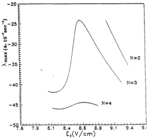
for all three cases. We write ±n(N)l (t) = ±n(N )l (0)e¸ t and substitute into Eq. (39) to solve for the eigenvalues of the matrix Mll(N )0 : There are 2s different eigenvalues of ¸l (jlj = 1; 2; ¢¢¢; s). If
all the real parts of the¸’s are negative, then the steady-state solution n(N )(x) is stable. In Fig. 8 we plot¸m ax vs. Ez forN = 2; 3, and 4, where ¸m ax is defined as
¸m ax = maxfRe[¸l]; jlj = 1; 2 : : : sg: (41)
We see that all ¸m ax < 0 for N = 2; 3, and 4, and therefore all the corresponding steady-state multifilamentary pattern solutions are stable.
Finally it may be worthwhile to say some words about the approach we use in the stability analysis. We use the Fourier series expansion method to treat the spatial dependent problem. This is a reasonable approach because the steady-state solutionn(N )(x) satisfies the periodic boundary conditions n(N )(¡ L
x) = n(N)(Lx) and dn(N)=dxj¡ Lx = dn(N )=dxjLx. Therefore n(N )(x) can
be considered as an infinite extended periodic function with periodicity2Lx. Moreover n(N )(x) is a smooth varying function (cf. Fig. 6), and therefore its Fourier series expansion is expected to converge rapidly, especially for small N . It seems reasonable for us to truncate the series for l > 10 (for N =2, 3, and 4) in the numerical calculation. One more point about the truncation
is that if no filamentary state is stable, then the final stable state is a no-filament state, i.e., the uniform electron density state, which consists of only l = 0 component. Therefore higher-l
components of ±n(N )l should not play important roles in the stability analysis of n(N )(x). This is because if a high-l component of ±n(N)l (t) is unstable and becomes larger and larger as time t increases, then the original filamentary state n(N )(x) will transform to another filamentary state which contains thel-component with a large l. This is in contradiction to the stability analysis of
the RD equation [4], which shows that no filamentary state is stable. Of course, the additional constraint in our theory may alter the above conclusion, and the truncation may not be a good approximation. But if this is the case, then it does no harm to our theory. Because filamentary states do exist, although it may become oscillatory states as studied in Ref. [6], in the large R
limit. However we believe that the truncation is a good approximation, and stable stationary mulitifilamentary states exist which is consistent with the experimental result of Ref. [2] in the smallR limit.
VI. Conclusions
We have established a theoretical model which can support stable steady-state mutifilamen-tary pattern solutions in SNDC semiconductors. This model is based on the basic equations in electrodynamics and the widely accepted two-trap-level models for the SNDC materials. There are no no extra assumptions in the model, and therefore we think that our model is simpler and more realistic than the existing models, which either needs an extra physical quantity to have stable steady-state solutions [5] or can not support stable steady-state solutions in the weak coupling (resistance R! 0) limit [6]. For completeness, stability analysis of the steady-state solutions is
given to show that these solutions are stable.
Acknowledgments
This work is supported in part by the National Science Council of the Republic of China under contract No. NSC 88-2112-M-002-002.
References
[ 1 ] B. K. Ridley, Proc. Phys. Soc. 82, 954 (1963).
[ 2 ] K. M. Mayer, J. Parisi, R. P. Huebener, Z. Phys. B 71, 171 (1988). [ 3 ] F. Schl¨ogl, Z. Phys. 253, 147 (1972).
[ 4 ] E. Sch¨oll, Z. Phys. B 62, 245 (1985).
[ 5 ] K. Kardell et al., J. Appl. Phys. 64, 1 (1988).
[ 6 ] A. Alekseev, S Bose, P. Rodin, and E. Sch¨oll, Phys. Rev. E 57, 2640 (1998).
[ 7 ] E. Sch¨oll, Nonequilibrium Phase Transitions in Semiconductors (Springer, Berlin, 1987). [ 8 ] J. Peinke et al., Encounter with Chaos (Spinger, Berlin, 1992).
[ 9 ] D. J. Robbins, Phys. Status Solidi (B) 97, 387 (1980). [10] W. Shockley, Solid State Electron. 2, 35 (1961).
![TABLE I. Typical material parameter values corresponding to n-GaAs at 4:2 ± K for the two-level generation-recombination mechanism [7]](https://thumb-ap.123doks.com/thumbv2/9libinfo/8858478.244529/6.892.152.807.259.543/table-typical-material-parameter-corresponding-generation-recombination-mechanism.webp)