FanXieZhaoTangYao GEOPHYSICS 2021 Optimal frequency domain discontinuous grid FD operator

(1)

For Peer Review

An optimal frequency-domain finite-difference operator with a flexible stencil and its application in

discontinuous-grid modeling

Journal: Geophysics

Manuscript ID GEO-2020-0296.R4 Manuscript Type: Technical Paper

Keywords: frequency-domain, 2D, finite difference, modeling, wave equation Manuscript Focus Area: Seismic Modeling and Wave Propagation

Downloaded 04/07/21 to 171.40.112.197. Redistribution subject to SEG license or copyright; see Terms of Use at http://library.seg.org/page/policies/terms

(2)

For Peer Review

1

An optimal frequency-domain finite-difference operator

2

with a flexible stencil and its application in

3

discontinuous-grid modeling

4

5 Na Fan1*_{, Xiao-Bi Xie}2_{, Lian-Feng Zhao}3_{, Xin-Gong Tang}1_{, Zhen-Xing Yao}3

6

7 Right Running Head: Frequency-domain FD modeling

8 9

10 1 _{Yangtze University, Key Laboratory of Exploration Technology for Oil and Gas}

11 Resources of Ministry of Education, Wuhan, China and Cooperative Innovation

12 Center of Unconventional Oil and Gas (Ministry of Education & Hubei Province),

13 Wuhan, China. E-mail: [email protected]; [email protected]

14 2 _{Institute of Geophysics and Planetary Physics, University of California at Santa}

15 Cruz, California, USA. E-mail: [email protected]

16 3 _{Key Laboratory of Earth and Planetary Physics, Institute of Geology and}

17 Geophysics, Chinese Academy of Sciences, Beijing, China. E-mail:

18 [email protected]; [email protected] 19 20 21 January 10, 2021 22 4 5 6 7 8 9 10 11 12 13 14 15 16 17 18 19 20 21 22 23 24 25 26 27 28 29 30 31 32 33 34 35 36 37 38 39 40 41 42 43 44 45 46 47 48 49 50 51 52 53 54 55 56 57 58 59

(3)

For Peer Review

23

ABSTRACT

24 We develop an optimal method to determine expansion parameters for flexible

25 stencils in 2D scalar wave finite-difference frequency-domain (FDFD) simulation.

26 The proposed stencil only requires the involved grid points to be paired and

27 rotationally symmetric around the central point. We apply this method to the

28 transition zone in discontinuous-grid modeling, where the key issue is designing

29 particular FDFD stencils to correctly propagate the wavefield passing through the

30 discontinuous interface. The proposed method can work in FDFD discontinuous-grid

31 with arbitrary integer coarse-to-fine gird spacing ratios. Numerical examples are

32 presented to demonstrate how to apply this optimal method for the discontinuous-grid

33 FDFD schemes with spacing ratios 3 and 5. The synthetic wavefields are highly

34 consistent to those calculated using the conventional dense uniform grid, while the

35 memory requirement and computational costs are greatly reduced. For velocity

36 models with large contrasts, the proposed discontinuous-grid FDFD method can

37 significantly improve the computational efficiency in forward modeling, imaging and

38 full waveform inversion.

4 5 6 7 8 9 10 11 12 13 14 15 16 17 18 19 20 21 22 23 24 25 26 27 28 29 30 31 32 33 34 35 36 37 38 39 40 41 42 43 44 45 46 47 48 49 50 51 52 53 54 55 56 57 58 59

(4)

For Peer Review

40

INTRODUCTION

41 Full-waveform inversion (FWI) is considered a promising technique for

42 retrieving the subsurface velocity structure. It heavily relies on forward modeling

43 during iterations in the optimization process. The modeling can be performed either in

44 the frequency or time domain. Frequency-domain FWI becomes attractive because it

45 can be naturally built into multiscale approaches to mitigate cycle-skipping,

46 conveniently handle independent frequencies and multishot computations, or easily

47 include the frequency-dependent attenuation. Another advantage is that the

48 frequency-domain method does not need to store wavefield values when calculating

49 the gradient (Vigh and Starr, 2008; Virieux and Operto, 2009). The frequency-domain

50 finite-difference (FDFD) forward modeling is an important part of frequency-domain

51 FWI. Great efforts have been made to develop optimal FDFD operators. Jo et al.,

52 (1996) propose the optimal nine-point scheme based on rotated FDFD operators.

53 Succeeding researchers extended this idea to other FDFD schemes such as acoustic

54 25- and 17-point schemes, and certain elastic and viscoelastic applications (e.g., Shin

55 and Sohn, 1998; Štekl and Pratt, 1998; Hustedt et al., 2004; Operto et al., 2007;

56 Operto et al., 2009; Cao and Chen, 2012; Operto et al., 2014). Min et al., (2000)

57 propose the weighted-average method to simplify the optimal procedure of Jo et al.,

58 (1996), which was later applied to other cases (e.g., Gu et al., 2013; Yang and Mao,

59 2016). Targeted to cases with different vertical and horizontal spacings, Chen, (2012)

60 proposed a new optimal nine-point scheme based on the average-derivative method

61 (ADM), and it has been extended to other cases (e.g., Tang et al., 2015; Zhang et al.,

62 2015; Chen and Cao, 2016, 2018). However, these optimized operators cannot be

63 easily expanded from the commonly-used nine-point scheme to other schemes with

64 different FDFD stencils. Therefore, similar to the finite-difference time-domain

4 5 6 7 8 9 10 11 12 13 14 15 16 17 18 19 20 21 22 23 24 25 26 27 28 29 30 31 32 33 34 35 36 37 38 39 40 41 42 43 44 45 46 47 48 49 50 51 52 53 54 55 56 57 58 59

(5)

For Peer Review

65 (FDTD) optimization operators (Holberg, 1987; Etgen, 2007; Wang et al., 2019a), a

66 general optimized FDFD operator was proposed by Fan et al., (2017) based on

67 solving the frequency-domain 2D scalar wave equation. Most of previous FDFD

68 schemes can be treated as special cases under this framework. In addition,

69 applications of this optimal procedure have been extended to more complicated cases

70 such as the 3D acoustic (Fan et al., 2018b) and elastic wave equations (Li et al.,

71 2018).

72 The FDFD is a computationally and memory intensive method (Plessix, 2009),

73 which prevents it from being widely used in the FWI. The nonuniform grid method,

74 which usually uses variable grid density to discretize models with large velocity

75 contrasts, was developed to mitigate this disadvantage (Wang et al., 2019c). The

76 nonuniform grid finite-difference (FD) modeling algorithms can be classified into two

77 groups. The first group uses continuous nonuniform grids that vary continuously

78 along certain coordinate (Falk et al., 1996; Moczo, 1989; Opršal and Zahradník, 1999;

79 Oliveira, 2003; Pitarka, 1999; Chu and Stoffa, 2012). The computation is usually very

80 convenient once the FD operator can be applied to rectangular grid. The second group

81 uses discontinuous nonuniform grids that are flexible in terms of discretizing the

82 model (Aoi and Fujiwara, 1999; Kristek et al., 2010; Zhang et al., 2013). It usually

83 can save more computational costs, but needs special treatment in the

84 fine-to-coarse-grid transition area (Jastram and Behle, 1992; Jastram and Tessmer,

85 1994; Wang et al., 2001; Fan et al., 2015). Similar nonuniform-grid techniques have

86 been widely used in FDTD modeling (e.g., Kang and Baag, 2004; Huang and Dong,

87 2009a, b; Liu et al., 2014; Nie et al., 2015; Fan et al., 2015; Wang et al., 2019c). For

88 the nonuniform-grid FDFD modeling, Li and Jia, (2018) develop a continuous-grid

89 FDFD modeling method based on the AMD FDFD operator of Chen (2012).

4 5 6 7 8 9 10 11 12 13 14 15 16 17 18 19 20 21 22 23 24 25 26 27 28 29 30 31 32 33 34 35 36 37 38 39 40 41 42 43 44 45 46 47 48 49 50 51 52 53 54 55 56 57 58 59

(6)

For Peer Review

90 However, compared to the continuous-nonuniform grid FDFD modeling, the

91 discontinuous-nonuniform grid method can discretize the model more flexibly and

92 save more costs. The major issue is in the fine-coarse grid transition zone, where

93 special FDFD operators need be designed to maintain the global accuracy of the wave

94 propagation. By using Fan et al. (2017)’s general FDFD optimal procedure, Fan et al.,

95 (2018a) proposed a discontinuous-grid FDFD method to transfer the wavefield cross

96 the fine-to-coarse transition zone without lowering the accuracy. But the spacing ratio

97 (N) was restricted to a power of two, which limited its practical applications.

98 In the following study, we develop a new optimal method with a flexible stencil for

99 2D scalar wave FDFD and apply it to the discontinuous-grid modeling. Theoretically,

100 with the new method, the coarse-to-fine spacing ratio N can be expanded to any

101 integer. In the rest part of this paper, we first introduce the optimal theory for

102 discontinuous-grid FDFD schemes, and investigate their dispersion relations and

103 structures of impedance matrixes. Then, we validate the proposed method using

104 numerical examples in discontinuous-grids and their results are compared with those

105 using traditional uniform-grid. Finally, a brief conclusion summarizes the advantage

106 of the proposed method.

107

108

METHODOLOGY

109

FDFD operator

110 The frequency-domain 2D scalar wave equation can be expressed as (Jo et al.,

111 1996) 112 2P₂ 2P₂ ₂2 P 0, (1) x z v   _ _ _   4 5 6 7 8 9 10 11 12 13 14 15 16 17 18 19 20 21 22 23 24 25 26 27 28 29 30 31 32 33 34 35 36 37 38 39 40 41 42 43 44 45 46 47 48 49 50 51 52 53 54 55 56 57 58 59 60

(7)

For Peer Review

113 where v is the model velocity, ω is the angular frequency, P is the pressure, and x

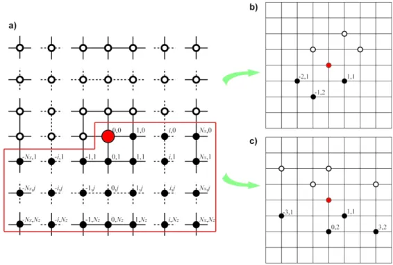
114 _{and are horizontal and vertical spatial coordinates. To introduce a flexible FDFD}z

115 stencil, we use the grid geometry shown in Figure 1, where Figure 1a is a general

116 stencil and Figure 1b and 1c are two sample stencils. The involved gridpoints have to

117 be paired and centrosymmetric. In other words, every grid point is the same as another

118 one located at 180°rotation. Therefore, we only need determine half of these points.

119 For the general FDFD stencil in Figure 1a, the commonly used 9- or 25-point scheme

120 can be considered as its special case. Similarly, we can form other stencils by

121 choosing certain points from the general stencil, or equivalently, setting weighting

122 coefficients to points of the general stencil (including using zero coefficients to

123 eliminate unwanted points) to form new stencils like in Figure 1b and 1c. Therefore,

124 we can unify our analyses to specific stencils by investigating the general stencil. We

125 use the general FDFD stencil in Figure 1a to approximate the two second-order spatial

126 derivatives _2_{P x}_ 2 and _2_{P z}_ 2 in equation 1. For the mass acceleration term

127 2 2 , we follow previous approaches (Jo et al., 1996; Min et al., 2000; Chen,

v P



128 2012; Fan et al., 2017) and approximate it using the weighted sum of all gridpoints

129 involved in the stencil and obtain

130 (2)





   









  , , , , , , 2 2 0 0 2 , , , 2 0 1 1 0, x x z z x z N N N N i j m i n j m i n j i j m i n j m i n j j i F j j i F j N N i j m i n j m i n j j i F j c P P d P P x z b P P v                           

 

131 where Pm n_, =P m x n z



 , 



, x and z are horizontal and vertical sampling

132 intervals. Subscripts i, j denote spatial locations in Figure 1a, and

4 5 6 7 8 9 10 11 12 13 14 15 16 17 18 19 20 21 22 23 24 25 26 27 28 29 30 31 32 33 34 35 36 37 38 39 40 41 42 43 44 45 46 47 48 49 50 51 52 53 54 55 56 57 58 59

(8)

For Peer Review

133

 

0 , if 0. , if 0 x j F j N j    _ _ 

134 The summation includes half of all gridpoints as circled by the red line in Figure 1a.

135 bi j, , ci j, and di j, are weighting coefficients for the mass acceleration term and two

136 spatial derivatives and they satisfy with ,   , 0 1 2 x z N N i j j i F j b   

 

bi j, 0   , 0 0 x z N N i j j i F j c   

 

137 and , respectively. When we set Nx=1, Nz=1 it becomes the   , 0 0 x z N N i j j i F j d   

 

138 commonly-used nine-point scheme, and when Nx=2, Nz=2 it is the 25-point scheme.

139 Other 2D FDFD schemes can also be considered as its special cases.

140 Similar to Fan et al. (2017), we separate the analysis of Δx≥Δz from Δx<Δz. Only

141 the former will be investigated and the latter can be analyzed by exchanging and x

142 z directions. In order to simplify equation 2, we define 2 , where

, , ,

i j i j i j

a c r d

143 r  x z is the aspect ratio. By substituting them into equation 2, we obtain

144





, (3)    





2 , , , , , , 2 2 0 0 1 0 x x z N z N N N i j m i n j m i n j i j m i n j m i n j j i F j j i F j a P P b P P x v                  

 

145 where a_{i j}_, satisfies .   , 0 0 x z N N i j j i F j a   

 

146 Next, the classical dispersion analysis is implemented to obtain the optimization

147 coefficients (Chen 2012; Fan et al., 2017). We substitute a monochromatic plane

148 wave P x z



, ,



P e₀ i k x k z x  z t into equation 3, where and are horizontal

x

k k_z

149 and vertical components of the wavenumber vector, and derive the normalized phase

150 velocity V_ph v as follows 4 5 6 7 8 9 10 11 12 13 14 15 16 17 18 19 20 21 22 23 24 25 26 27 28 29 30 31 32 33 34 35 36 37 38 39 40 41 42 43 44 45 46 47 48 49 50 51 52 53 54 55 56 57 58 59

(9)

For Peer Review

151   , (4)   , , 0 , , 0 2 x z x z N N i j i j j i F j ph N N i j i j j i F j a T V G v b T       

 

152 where G is the number of grid points per wavelength, which is defined with respect to

153 the larger spatial interval, and T_{i j}_, cos i2 sin j2 cos , and is the

G rG

   

 

 _  _

  

154 propagation angle relative to the vertical axis. Then, we minimize the following phase

155 error function to obtain optimized a_{i j}_, and b_{i j}_, ,

156





, (5) 2 , , , 1 ph i j i j V E a b dkd v     _  _  



% 157 where k%1G.

158 Coefficients c_{i j}_, and d_{i j}_, are also required when the absorbing boundary such as

159 the widely used perfectly matched layer (PML) is used. Following the approach by

160 Fan et al. (2018a), these coefficients can be determined by minimizing the error

161 function, 162







2 2



, (6) , , , 1 2 i j i j E c d 



E E dkd% 163 Where 164 , (7a)     2 1 , , , , 0 0 2 sin + x x z N z N N N i j i j i j i j j i F j j i F j E c T b T G          _ _  

 

165 and 166 . (7b)     2 2 , , , , 0 0 2 cos + x x z N z N N N i j i j i j i j j i F j j i F j E d T b T rG          _ _  

 

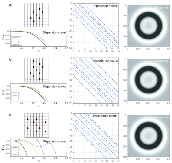
167 As examples, we use the above procedure to calculate optimal coefficients for three

168 FDFD operators shown in Figure 2. The optimized coefficients are listed in Table 1.

169 The general features of these operators are compared in Figure 2, including dispersion

4 5 6 7 8 9 10 11 12 13 14 15 16 17 18 19 20 21 22 23 24 25 26 27 28 29 30 31 32 33 34 35 36 37 38 39 40 41 42 43 44 45 46 47 48 49 50 51 52 53 54 55 56 57 58 59

(10)

For Peer Review

170 curves and structures of impedance matrixes. The structures of matrixes are related to

171 the FDFD stencils, and they have lager bandwidths along the diagonals comparing to

172 the conventional standard nine-point operator in Jo et al., (1996). To validate the

173 schemes, we further simulate the scalar wave propagation in a 2D homogeneous

174 media using these schemes. Their snapshots are also shown in Figure 2. The

175 dispersion curves of these three stencils show different accuracies, in which stencils in

176 Figure 2a and 2b have similar accuracies because 2b has only one more pair of

177 gridpoints than 2a and these two additional gridpoints stay far from the central

178 gridpoint, thus do not affect the accuracy too much. Stencil in Figure 2c has the

179 lowest accuracy because its gridpoints are more unevenly distributed and some of

180 them stay far away from the central gridpoint. From Figure 2 we conclude that the

181 accuracy of a FDFD operator is related to the shape and number of points involved in

182 a stencil. Similar tests are conducted using other FDFD stencils although their results

183 are not shown here. These numerical examples demonstrate that, if more points are

184 involved, or points are distributed more evenly, or points are closer to the central

185 point, the resulted FD stencil tends to be more accurate.

186

187

Discontinuous-grid modeling

188 The subsurface velocity usually increases with the depth. To adapt to velocity

189 variations and reduce the computation cost, a variable grid is often desirable. Fan et

190 al., (2018a) propose a discontinuous-grid FDFD method. However, it only works for

191 the coarse-to-fine grid spacing ratio N 2, or for _N _2n by using the procedure n

4 5 6 7 8 9 10 11 12 13 14 15 16 17 18 19 20 21 22 23 24 25 26 27 28 29 30 31 32 33 34 35 36 37 38 39 40 41 42 43 44 45 46 47 48 49 50 51 52 53 54 55 56 57 58 59

(11)

For Peer Review

192 times, where n is a positive integer. Here we present a general discontinuous-grid

193 method which can be used for arbitrary integer N. In general, N can be

194 determined by the ratio of velocities across the transition zone, e.g., we can use

195 discontinuous-grid with N 2 if the velocity doubles. Considering the actual

196 velocity contrast involved, discontinuous-grids with N  2 5 are the most useful.

197 Since cases N  2 and N  4 have been covered by Fan et al., (2018a), here we

198 only discuss cases N 3_and N 5, although the current procedure can be applied

199 to an arbitrary integer N .

200 Since the standard nine-point operator is one of the most widely used FDFD

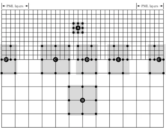
201 schemes, we take it as the example to demonstrate the discontinuous-grid FDFD

202 modeling. We first present the methodology for the discontinuous-grid scheme with

203 N 3 shown in Figure 3. Assuming the model has lower and higher velocities in

204 shallow and deep area, and the higher speed is at least three times of the lower speed,

205 _{we grid the model by ∆x and ∆z in the upper part and 3∆x and 3∆z in the lower part.} 206 The fine grid should cover the entire low-velocity area and extend into the

207 high-velocity area for at least 3∆z to ensure the accuracy of the wavefield crossing the

208 transition zone. If other stencils are used, the size of the overlapped zone may be

209 different. For example, for the 25-point stencil, the overlapped zone should be at least

210 6∆z. Figure 3 shows several typical FDFD stencils involved in fine-grid, coarse-grid

211 and transition areas. In regular-grid areas including both fine- and coarse-grids,

212 standard nine-point operators are used as illustrated by gridpoints A and B in Figure

213 3. While in the connecting row, FDFD operators with special stencils are used to

4 5 6 7 8 9 10 11 12 13 14 15 16 17 18 19 20 21 22 23 24 25 26 27 28 29 30 31 32 33 34 35 36 37 38 39 40 41 42 43 44 45 46 47 48 49 50 51 52 53 54 55 56 57 58 59

(12)

For Peer Review

214 ensure the wavefield continuity across that row. The connecting row involves three

215 kinds of gridpoints. One is the gridpoint C, where standard nine-point operator works.

216 The other two are gridpoints D and E, where new nine-point operators are designed

217 based on the distribution of surrounding points. The FDFD stencils at D and E are

218 mirrored about the vertical line, therefore we only need calculating optimal

219 coefficients for one of them.

220 When the FD stencil reaches to the absorbing boundary, the requirement of

221 rotationally symmetry around the central point may not be satisfied. Under this

222 circumstance, we simply omit the gridpoints outside the boundary, and use distorted

223 stencils such as D’ and E’ shown in Figure 3. For simplicity, their optimal coefficients

224 are still determined using the full stencils D and E. Numerical tests verified, because

225 of the existing absorbing condition, the wavefield is very weak when bouncing back

226 from the boundary. Therefore, this simple boundary treatment does not affect the

227 result too much, and high accuracy wavefield can still be achieved.

228 The coefficients for FDFD schemes at D or E can be obtained following the

229 _{optimization procedure in the previous section. The range of is set within [0, 0.08]}k%

230 by the tradeoff between the minimum G and the phase velocity error. Table 2 lists the

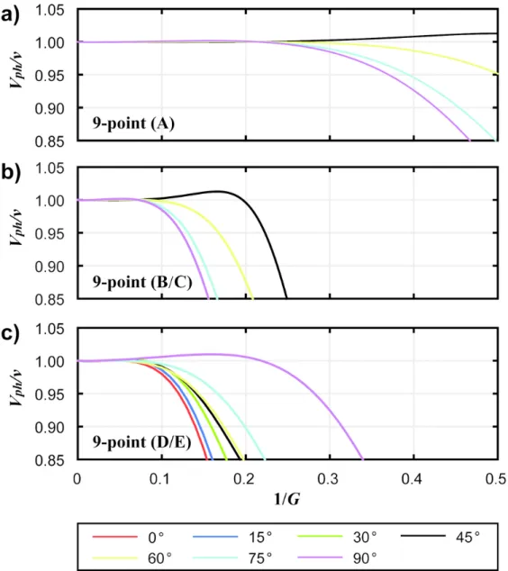
231 resulting optimal coefficients of nine-point operator at D/E. Figure 4 shows the

232 normalized phase velocities (dispersion curves) for all FDFD operators in Figure 3.

233 Taking the commonly used 1% criterion for the minimum G, i.e. keeping the

234 threshold of normalized phase velocity as 0.99, we find the maximum values of 1 G

235 for operators at gridpoints A, B/C and D/E are 0.29, 0.097 and 0.1 respectively.

4 5 6 7 8 9 10 11 12 13 14 15 16 17 18 19 20 21 22 23 24 25 26 27 28 29 30 31 32 33 34 35 36 37 38 39 40 41 42 43 44 45 46 47 48 49 50 51 52 53 54 55 56 57 58 59

(13)

For Peer Review

236 However, operators B-E fall into regions where the speed is at least 3 times faster

237 (i.e., the wavelength is at least 3 times longer), the maximum values of 1 G are

238 actually 0.29, 0.29 and 0.3. Therefore, for the nine-point discontinuous-grid scheme

239 with N 3, the G should be at least 3.44 in order to limit the phase velocity error

240 within 1%.

241 Similarly, we consider the discontinuous-grid scheme with N 5, where the

242 high speed in the lower area is at least 5.0x as the low speed in the upper area. Figure

243 5 shows several typical FDFD stencils used in fine-grid, coarse-grid and transition

244 areas. We use standard nine-point operators in regular grid areas. In the connecting

245 row, there are five different FDFD operators (Figure 5). The first one is the gridpoint

246 located at the continuous vertical grid line (indicated by C) where the standard

247 nine-point operator can work. Other two types are the gridpoints located at

248 discontinuous vertical grid lines (indicated by D and G), where two symmetrical

249 13-point schemes are used. The last two are the gridpoints located at the

250 discontinuous vertical grid lines (indicated by E and F) where two symmetrical

251 11-point schemes are used.

252 The coefficients for FDFD operators at D/G and E/F can also be calculated by

253 optimizing the objective functions 5 and 6. The range of is set within [0, 0.05] and k%

254 Table 3 lists the resulting coefficients. Figure 6 shows the normalized phase velocities

255 for all FDFD operators in Figure 5. Similarly, we find the maximum values of 1/G

256 within 1% phase velocity error for operators in Figures 6a-6d are 0.29, 0.058, 0.06

257 and 0.06, respectively. Since operators B-G fall into the high-speed area, the

4 5 6 7 8 9 10 11 12 13 14 15 16 17 18 19 20 21 22 23 24 25 26 27 28 29 30 31 32 33 34 35 36 37 38 39 40 41 42 43 44 45 46 47 48 49 50 51 52 53 54 55 56 57 58 59

(14)

For Peer Review

258 maximum values of 1 G are actually 0.29, 0.29, 0.30 and 0.30, respectively. So for

259 the nine-point discontinuous-grid scheme with N=5, the G should be larger than 3.44

260 to limit the phase velocity error within 1%.

261 The FDFD forward modeling is calculated by solving the linear system AU=S,

262 where A is the impedance matrix, U is the wavefield and S is the source. The size and

263 sparsity of the impedance matrix A primarily determine the computational efficiency

264 (Štekl and Pratt, 1998). As an example, we use a simple model to compare the

265 impedance matrices of the uniform and discontinuous grids with N=3 and N=5. The

266 model is partitioned in three ways, a uniform grid composed of 31 × 21 grid points

267 (Figure 7a), a N=3 discontinuous grid consisting of 31 × 6 grid points in the top layer

268 and 11 × 5 grid points in the bottom layer (Figure 7c), and another N=5 discontinuous

269 grid consisting of 31 × 6 grid points in the top layer and 7 × 3 grid points in the

270 bottom layer (Figure 7e). The structures of their impedance matrices are compared in

271 Figures 7b, 7d and 7f. Compared with the uniform grid, the discontinuous gird

272 reduces the size of the impedance matrix to 37% for N=3 and 32% for N=5; reduces

273 the nonzero elements to 36% for N=3 and 32% for N=5, respectively. For both

274 discontinuous-gird schemes, the size and sparsity of the impedance matrix are greatly

275 reduced.

276 In general, with the methodology presented above, we can build discontinuous-grid

277 FDFD scheme with an arbitrary N. What we should do is designing accurate FDFD

278 stencils in the fine-to-coarse connecting region according to the distribution of

279 surrounding grid points, followed by using the above-mentioned method to optimize

4 5 6 7 8 9 10 11 12 13 14 15 16 17 18 19 20 21 22 23 24 25 26 27 28 29 30 31 32 33 34 35 36 37 38 39 40 41 42 43 44 45 46 47 48 49 50 51 52 53 54 55 56 57 58 59

(15)

For Peer Review

280 expansion coefficients and examine their accuracy. The resulted FDFD schemes can

281 reduce the computation cost while still maintaining the required accuracy.

282

283

NUMERICAL EXAMPLES

284 In this section, we present three numerical experiments to test the proposed

285 discontinuous-grid FDFD scheme. We implement these simulations using two simple

286 and one complex models. Comparisons between different results, including snapshots

287 and waveforms obtained by our schemes and the traditional uniform-grid scheme, are

288 used to demonstrate the accuracy and efficiency of the proposed scheme.

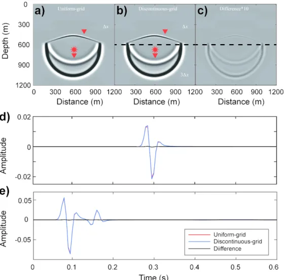
289 We first validate the discontinuous-grid FDFD scheme with N=3 using a two-layer

290 model. The model has a size of 1200×1200 m2 _{and velocities of 1000 m/s and 3000}

291 m/s in the top and bottom layers, respectively. The velocity interface is at z=575 m. A

292 30-Hz Ricker wavelet source is used in this and the following examples, and is

293 injected at (600, 400) m (indicated by red stars in Figures 8a and 8b). Both the

294 uniform-grid scheme and discontinuous-grid schemes are used in the simulation. The

295 former uses a small spatial interval of    x z 2.5 m to discretize the entire model

296 and results a grid size of 481 × 481. The latter uses a small spatial interval of

297    x z 2.5 m to discretize the upper area above z600 m (indicated by a

298 dashed line in Figure 8b) to guarantee the transition grids all fall in the high-speed

299 region. The rest area is discretized by a large spatial interval of 3 x and 3 z . The

300 resulting fine- and coarse-grid points are 481×241 and 161×80 respectively. A PML

301 absorbing boundary is used in this and the following two examples (Tang et al., 2015;

4 5 6 7 8 9 10 11 12 13 14 15 16 17 18 19 20 21 22 23 24 25 26 27 28 29 30 31 32 33 34 35 36 37 38 39 40 41 42 43 44 45 46 47 48 49 50 51 52 53 54 55 56 57 58 59

(16)

For Peer Review

302 Fan et al., 2017; Wang et al., 2019b). Two receivers are placed at (750, 400) m and

303 (600, 750) m, with one in the low-speed region and the other in the high-speed region

304 (indicated by reversed triangles in Figures 8a and 8b). The G value is 4.44 for both the

305 uniform and the discontinuous schemes if we assume the shortest wavelength is one

306 third of the dominant wavelength of a Ricker wavelet. Simulation results are shown in

307 Figure 8, where wavefield snapshots (Figures 8a and 8b) are both at 0.4 s and

308 synthetic seismograms are compared at two receivers (Figures 8d and 8e). To

309 demonstrate the accuracy of the synthetic wavefield, the differential snapshot is

310 amplified by 10x and shown in Figure 8c, and differential seismograms are

311 overlapped in Figures 8d and 8e. The slightly polygonal shaped waveform compared

312 to the usual FDTD result is due to they have different time sampling interval. In a

313 FDTD, it is determined by the stability criterion, while in a FDFD it is determined by

314 the sampling principle which requires two samples per period for the highest

315 frequency. The former is usually much smaller than the latter, although they actually

316 have the same accuracy.

317 To validate the case in which the source is located in the coarse grid zone, we

318 conduct a similar calculation by moving the source to (600, 675) m. The

319 corresponding results are shown in Figure 9. The results in Figures 8 and 9

320 demonstrate that both uniform- and discontinuous-grids generate comparable

321 accuracy. Regarding computational costs, it is mainly dependent on the structure of

322 the complex-valued impedance matrix due to implicitly solving the large sparse linear

323 equations. The computational times on a single CPU 4-core (Intel Core i7-4790)

4 5 6 7 8 9 10 11 12 13 14 15 16 17 18 19 20 21 22 23 24 25 26 27 28 29 30 31 32 33 34 35 36 37 38 39 40 41 42 43 44 45 46 47 48 49 50 51 52 53 54 55 56 57 58 59

(17)

For Peer Review

324 desktop needed for uniform- and discontinuous-grid modelings are 774 and 229 s

325 respectively because the latter reduces both the number of nonzero elements and the

326 size of the matrix to 56% for this specific numerical experiment.

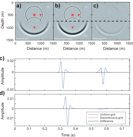
327 We use the next two-layer model to validate the discontinuous-grid FDFD

328 method under _N _₅. The model has a size of 1500 × 1500 m2_{. The velocities are}

329 1000 m/s and 5000 m/s in the top and bottom layers, with an interface at z=725 m.

330 The source is located at (750, 500) m. For the uniform-grid scheme, we use a small

331 spatial interval of ∆x=∆z=2.5 m to discretize the entire model and obtain a grid size of

332 601 × 601. For discontinuous-grid scheme, we use a small spatial interval of

333 ∆x=∆z=2.5 m to discretize the area above z=750 m (indicated by a dashed line in

334 Figure 10b) and a large spatial interval of 5Δx and 5Δz to discretize the rest area. The

335 gridpoints of the finely- and coarsely-gridded areas are 601×301 and 121×60. Two

336 receivers are placed at (1000, 500) m and (750, 1000) m, with one in the low-speed

337 region and the other in the high-speed region (Figure 10b). Simulation results from

338 these two different schemes are compared in Figure 10. Figures 10a and 10b compare

339 the wavefield snapshots at 4.0 s, and shown in Figure 10c is their differential snapshot

340 amplified by 10x. Figures 10d and 10e compare synthetic seismograms from two

341 receivers. Regarding the computational costs, the computational times on a single

342 CPU 4-core (Intel Core i7-4790) desktop needed for uniform- and discontinuous-grid

343 modeling are 787 and 429 s, respectively, because the latter reduces both the number

344 of nonzero elements and the size of impedance matrix to 52%.

345 In the last example, to better test the proposed discontinuous-grid method in a more

4 5 6 7 8 9 10 11 12 13 14 15 16 17 18 19 20 21 22 23 24 25 26 27 28 29 30 31 32 33 34 35 36 37 38 39 40 41 42 43 44 45 46 47 48 49 50 51 52 53 54 55 56 57 58 59

(18)

For Peer Review

346 realistic model having large velocity contrast, we convert part of the Marmousi2

347 Model (Martin et al., 2006) using

 

2

 

, where _{is the original} 0

, ,

P P

v x z Cv x z vP0

348 velocity, v_P is the converted velocity, and C 0.25s km is a constant. The

349 resulted velocity model with a size of 1903×1220 m2_{is showed in Figure 11a. The}

350 source and four receivers are located at (950,100) m, (550,100) m, (1268,802) m,

351 (954,1038) m and (634,1120) m, respectively (Figure 11a). Figure 11b show velocity

352 versus depth curves at distances x=0 and x=1903 m. The velocity generally increases

353 with the depth but there is a high-velocity salt layer close to the bottom of the model.

354 To apply the discontinuous-grid method, we separate the entire model into four layers

355 and use different grid density to discretize the model. The depth ranges for these

356 layers are 0-703m, 703-1009 m, 1009-1081 m and 1081-1220 m, with corresponding

357 minimum velocities 682.4 m/s, 1572.8 m/s, 4497.2 m/s and 1930.1 m/s (Figure 11b),

358 respectively. Based on their velocity variation ranges, we grid these regions by ∆x,

359 2∆x, 6∆x and 2∆x, respectively, where  x 1m. The spacing ratios at boundaries

360 between the lower and upper layers are N=2 at z=703 m, N=3 at z=1009 m and N=1/3

361 (or N=3 for upper to lower layer ratio) at z=1081 m.

362 For comparison, we also generate a set of results using the conventional

363 uniform-grid with ∆x=∆z=1 m. Figures 11c and 11d are snapshots at 1.0 s using both

364 uniform- and discontinuous-grid schemes. Figure 11e shows the differential snapshot

365 which is amplified by 10x. Figures 11f-11i compare synthetic seismograms from four

366 receivers located in different layers, with their differences overlapped to these

367 waveforms. For this complex model, the discontinuous-grid modeling reduces the

4 5 6 7 8 9 10 11 12 13 14 15 16 17 18 19 20 21 22 23 24 25 26 27 28 29 30 31 32 33 34 35 36 37 38 39 40 41 42 43 44 45 46 47 48 49 50 51 52 53 54 55 56 57 58 59

(19)

For Peer Review

368 impedance matrix to 67%, and the computational time on a dual CPU 2×8-core (Intel

369 Xeon E5-2630) machine from 7625 s to 4856 s comparing to the corresponding

370 uniform-grid modeling.

371 By comparing snapshots and synthetic seismograms in the above three numerical

372 examples, the results demonstrated that the discontinuous-grid scheme generates

373 highly consistent waveforms in simulating wave propagations while greatly reduces

374 the computational cost compared to the uniform-grid scheme.

375

376

CONCLUSION

377 We proposed an optimal method for discontinuous-grid FDFD operators with

378 flexible stencils. This method can be applied to arbitrary integer coarse-to-fine

379 spacing ratio N, given the involved grid points are properly paired and

380 centrosymmetric around the central point. Considering the spacing ratio N=2-5 is the

381 most commonly encountered situation, the proposed method should be very useful in

382 building discontinuous-grid FDFD simulations in high-contrast velocity structures for

383 reducing the computational time and memory cost while still maintaining the

384 accuracy. To demonstrate the application of this method, we applied it to irregular

385 FDFD stencils in connection regions with spacing ratios N=3 and N=5. Many detailed

386 procedures, e.g., designing irregular stencils, building objective functions, optimizing

387 expansion coefficients and analyzing dispersion curves and impedance matrixes, were

388 introduced. Numerical experiments in complex high-contrast velocity models were

389 calculated using the discontinuous-grid FDFD optimized with the proposed method.

4 5 6 7 8 9 10 11 12 13 14 15 16 17 18 19 20 21 22 23 24 25 26 27 28 29 30 31 32 33 34 35 36 37 38 39 40 41 42 43 44 45 46 47 48 49 50 51 52 53 54 55 56 57 58 59

(20)

For Peer Review

390 The snapshots and waveforms calculated with these schemes have accuracies

391 comparable to those using dense conventional uniform-grid schemes, while

392 computational costs were greatly reduced.

393

394 ACKNOWLEDGMENTS

395 The authors thank Jeffrey Shragge, Stig Hestholm, Wei Zhang and other three

396 anonymous reviewers for their critical comments that greatly improved this

397 manuscript. This research is financially supported by the National Natural Science

398 Foundation of China (grant nos. 41604037, 41630210, 41874119 and 41674107) and

399 the Open Fund of the Cooperative Innovation Center of Unconventional Oil and Gas

400 (Ministry of Education & Hubei Province) (No. UOG2020-09).

401

402

REFERENCES

403 Aoi, S., and H. Fujiwara, 1999, 3D finite-difference method using discontinuous grids: Bulletin of the 404 Seismological Society of America, 89, no. 4, 918-930.

405 Cao, S.-H., and J.-B. Chen, 2012, A 17-point scheme and its numerical implementation for 406 high-accuracy modeling of frequency-domain acoustic equation: Chinese Journal of 407 Geophysics, 55, no. 10, 3440-3449. doi: 10.6038/j.issn.0001-5733.2012.10.027.

408 Chen, J.-B., 2012, An average-derivative optimal scheme for frequency-domain scalar wave equation: 409 Geophysics, 77, no. 6, T201-T210. doi: 10.1190/geo2011-0389.1.

410 Chen, J.-B., and J. Cao, 2016, Modeling of frequency-domain elastic-wave equation with an 411 average-derivative optimal method: Geophysics, 81, no. 6, T339-T356. doi: 412 10.1190/geo2016-0041.1.

413 Chen, J.-B., and J. Cao, 2018, An average-derivative optimal scheme for modeling of the 414 frequency-domain 3D elastic wave equationAn optimal scheme for elastic equation: 415 Geophysics, 83, no. 4, T209-T234. doi: 10.1190/geo2017-0641.1.

416 Chu, C., and P. L. Stoffa, 2012, Nonuniform grid implicit spatial finite difference method for acoustic 417 wave modeling in tilted transversely isotropic media: Journal of Applied Geophysics, 76, 418 44-49. doi: 10.1016/j.jappgeo.2011.09.027.

419 Etgen, J. T., 2007, A tutorial on optimizing time domain finite-difference schemes:“Beyond Holberg”, 420 Stanford Exploration Project Report, 129, 33-43.

4 5 6 7 8 9 10 11 12 13 14 15 16 17 18 19 20 21 22 23 24 25 26 27 28 29 30 31 32 33 34 35 36 37 38 39 40 41 42 43 44 45 46 47 48 49 50 51 52 53 54 55 56 57 58 59

(21)

For Peer Review

421 Falk, J., E. Tessmer, and D. Gajewski, 1996, Tube wave modeling by the finite-difference method with 422 varying grid spacing: Pure and Applied Geophysics, 148, no. 1-2, 77-93. doi: 423 10.1016/j.jappgeo.2011.09.027.

424 Fan, N., L.-F. Zhao, Y.-J. Gao, and Z.-X. Yao, 2015, A discontinuous collocated-grid implementation for 425 high-order finite-difference modeling: Geophysics, 80, no. 4, T175-T181. doi: 426 10.1190/geo2015-0001.1.

427 Fan, N., L.-F. Zhao, X.-B. Xie, and Z.-X. Yao, 2018a, A discontinuous-grid finite-difference scheme for 428 frequency-domain 2D scalar wave modeling: Geophysics, 83, no. 4, T235-T244. doi: 429 10.1190/geo2017-0535.1.

430 Fan, N., L.-F. Zhao, X.-B. Xie, X.-G. Tang, and Z.-X. Yao, 2017, A general optimal method for 2D 431 frequency-domain finite-difference solution of scalar wave equation: Geophysics, 82, no. 3, 432 T121-T132. doi: 10.1190/geo2016-0457.1.

433 Fan, N., J.-W. Cheng, L. Qin, L.-F. Zhao, X.-B. Xie, and Z.-X. Yao, 2018b, An optimal method for 434 frequency-domain finite-difference solution of 3D scalar wave equation: Chinese Journal of 435 Geophysics, 61, no. 3, 1095-1108. doi: 10.6038/cjg2018L0375.

436 Gu, B., G. Liang, and Z. Li, 2013, A 21-point finite difference scheme for 2D frequency-domain elastic 437 wave modelling: Exploration Geophysics, 44, no. 3, 156-166. doi: 10.1071/EG12064.

438 Holberg, O., 1987, Computational aspects of the choice of operator and sampling interval for 439 numerical differentiation in large ‐ scale simulation of wave phenomena: Geophysical 440 prospecting, 35, no. 6, 629-655.

441 Huang, C., and L.-G. Dong, 2009a, High-order finite-difference method in seismic wave simulation with 442 variable grids and local time-steps: Chinese Journal of Geophysics, 52, no. 1, 176-186.

443 Huang, C., and L.-G. Dong, 2009b, Staggered-grid high-order finite-difference method in elastic wave 444 simulation with variable grids and local time-steps: Chinese Journal of Geophysics, 52, no. 11, 445 2870-2878. doi: 10.3969/j.issn.0001-5733.2009.11.022.

446 Hustedt, B., S. Operto, and J. Virieux, 2004, Mixed-grid and staggered-grid finite-difference methods 447 for frequency-domain acoustic wave modelling: Geophysical Journal International, 157, no. 448 3, 1269-1296. doi: 10.1111/j.1365-246X.2004.02289.x.

449 Jastram, C., and A. Behle, 1992, Acoustic modelling on a grid of vertically varying spacing: Geophysical 450 prospecting, 40, no. 2, 157-169. doi: 10.1111/j.1365-2478.1992.tb00369.x.

451 Jastram, C., and E. Tessmer, 1994, Elastic modelling on a grid with vertically varying spacing: 452 Geophysical prospecting, 42, no. 4, 357-370. doi: 10.1111/j.1365-2478.1994.tb00215.x. 453 Jo, C.-H., C. Shin, and J. H. Suh, 1996, An optimal 9-point, finite-difference, frequency-space, 2-D scalar 454 wave extrapolator: Geophysics, 61, no. 2, 529-537. doi: 10.1190/1.1443979.

455 Kang, T.-S., and C.-E. Baag, 2004, Finite-Difference Seismic Simulation Combining Discontinuous Grids 456 with Locally Variable Timesteps: Bulletin of the Seismological Society of America, 94, no. 1, 457 207-219. doi: 10.1785/0120030080.

458 Kristek, J., P. Moczo, and M. Galis, 2010, Stable discontinuous staggered grid in the finite-difference 459 modelling of seismic motion: Geophysical Journal International, 183, no. 3, 1401-1407. doi: 460 10.1111/j.1365-246X.2010.04775.x.

461 Li, A., H. Liu, Y. Yuan, T. Hu, and X. Guo, 2018, Modeling of frequency-domain elastic-wave equation 462 with a general optimal scheme: Journal of Applied Geophysics, 159, 1-15. doi: 463 10.1016/j.jappgeo.2018.07.014.

464 Li, Q., and X. Jia, 2018, A generalized average-derivative optimal finite-difference scheme for 2D 4 5 6 7 8 9 10 11 12 13 14 15 16 17 18 19 20 21 22 23 24 25 26 27 28 29 30 31 32 33 34 35 36 37 38 39 40 41 42 43 44 45 46 47 48 49 50 51 52 53 54 55 56 57 58 59

(22)

For Peer Review

465 frequency-domain acoustic-wave modeling on continuous nonuniform grids: Geophysics, 83, 466 no. 5, T265-T279. doi: 10.1190/geo2017-0132.1.

467 Liu, X., X. Yin, and G. Wu, 2014, Finite-difference modeling with variable grid-size and adaptive 468 time-step in porous media: Earthquake Science, 27, no. 2, 169-178. doi: 469 10.1007/s11589-013-0055-7.

470 Min, D.-J., C. Shin, B.-D. Kwon, and S. Chung, 2000, Improved frequency-domain elastic wave 471 modeling using weighted-averaging difference operators: Geophysics, 65, no. 3, 884-895. 472 doi: 10.1190/1.1444785.

473 Moczo, P., 1989, Finite-difference technique for SH-waves in 2-D media using irregular 474 grids—application to the seismic response problem: Geophysical Journal International, 99, 475 no. 2, 321-329. doi: 10.1111/j.1365-246X.1989.tb01691.x.

476 Nie, S., Y. Wang, K. Olsen, and S. Day, 2015, Stable Discontinuous Staggered Finite Difference Method 477 for Elastic Wave Simulations: 85th Annual International Meeting, SEG, Expanded Abstracts, 478 3774-3778.

479 Oliveira, S. A. M., 2003, A fourth-order finite-difference method for the acoustic wave equation on 480 irregular grids: Geophysics, 68, no. 2, 672-676. doi: 10.1190/1.1567237.

481 Operto, S., J. Virieux, A. Ribodetti, and J. E. Anderson, 2009, Finite-difference frequency-domain 482 modeling of viscoacoustic wave propagation in 2D tilted transversely isotropic (TTI) media: 483 Geophysics, 74, no. 5, T75-T95. doi: 10.1190/1.3157243.

484 Operto, S., J. Virieux, P. Amestoy, J.-Y. L’Excellent, L. Giraud, and H. B. H. Ali, 2007, 3D finite-difference 485 frequency-domain modeling of visco-acoustic wave propagation using a massively parallel 486 direct solver: A feasibility study: Geophysics, 72, no. 5, SM195-SM211. doi: 487 10.1190/1.2759835.

488 Operto, S., R. Brossier, L. Combe, L. Métivier, A. Ribodetti, and J. Virieux, 2014, Computationally 489 efficient three-dimensional acoustic finite-difference frequency-domain seismic modeling in 490 vertical transversely isotropic media with sparse direct solver: Geophysics, 79, no. 5, 491 T257-T275. doi: 10.1190/geo2013-0478.1.

492 Opršal, I., and J. Zahradník, 1999, Elastic finite-difference method for irregular grids: Geophysics, 64, 493 no. 1, 240-250. doi: 10.1190/1.1444520.

494 Pitarka, A., 1999, 3D elastic finite-difference modeling of seismic motion using staggered grids with 495 nonuniform spacing: Bulletin of the Seismological Society of America, 89, no. 1, 54-68. 496 Plessix, R.-É., 2009, Three-dimensional frequency-domain full-waveform inversion with an iterative 497 solver: Geophysics, 74, no. 6, WCC149-WCC157. doi: 10.1190/1.3211198.

498 Shin, C., and H. Sohn, 1998, A frequency-space 2-D scalar wave extrapolator using extended 25-point 499 finite-difference operator: Geophysics, 63, no. 1, 289-296. doi: 10.1190/1.1444323.

500 Štekl, I., and R. G. Pratt, 1998, Accurate viscoelastic modeling by frequency-domain finite differences 501 using rotated operators: Geophysics, 63, no. 5, 1779-1794. doi: 10.1190/1.1444472.

502 Tang, X., H. Liu, H. Zhang, L. Liu, and Z. Wang, 2015, An adaptable 17-point scheme for high-accuracy 503 frequency-domain acoustic wave modeling in 2D constant density media: Geophysics, 80, no. 504 6, T211-T221. doi: 10.1190/geo2014-0124.1.

505 Vigh, D., and E. W. Starr, 2008, Comparisons for waveform inversion, time domain or frequency 506 domain?: 78th Annual International Meeting, SEG, Expanded Abstracts, 1890-1894.

507 Virieux, J., and S. Operto, 2009, An overview of full-waveform inversion in exploration geophysics: 508 Geophysics, 74, no. 6, WCC1-WCC26. doi: 10.1190/1.3238367.

4 5 6 7 8 9 10 11 12 13 14 15 16 17 18 19 20 21 22 23 24 25 26 27 28 29 30 31 32 33 34 35 36 37 38 39 40 41 42 43 44 45 46 47 48 49 50 51 52 53 54 55 56 57 58 59

(23)

For Peer Review

509 Wang, E., J. Ba, and Y. Liu, 2019a, Temporal High-Order Time–Space Domain Finite-Difference 510 Methods for Modeling 3D Acoustic Wave Equations on General Cuboid Grids: Pure Applied 511 Geophysics, 176, no. 12, 5391-5414. doi: 10.1007/s00024-019-02277-2.

512 Wang, E., J. M. Carcione, J. Ba, M. Alajmi, and A. N. Qadrouh, 2019b, Nearly perfectly matched layer 513 absorber for viscoelastic wave equations: Geophysics, 84, no. 5, T335-T345. doi: 514 10.1190/geo2018-0732.1.

515 Wang, Y., J. Xu, and G. T. Schuster, 2001, Viscoelastic Wave Simulation in Basins by a Variable-Grid 516 Finite-Difference Method: Bulletin of the Seismological Society of America, 91, no. 6, 517 1741-1749. doi: 10.1785/0120000236.

518 Wang, Z.-Y., J.-P. Huang, D.-J. Liu, Z.-C. Li, P. Yong, and Z.-J. Yang, 2019c, 3D variable-grid 519 full-waveform inversion on GPU: Petroleum Science, 16, no. 5, 1001-1014. doi: 520 10.1007/s12182-019-00368-2.

521 Yang, Q., and W. Mao, 2016, Simulation of seismic wave propagation in 2-D poroelastic media using 522 weighted-averaging finite difference stencils in the frequency–space domain: Geophysical 523 Journal International, 208, no. 1, 148-161. doi: 10.1093/gji/ggw380.

524 Zhang, H., B. Zhang, B. Liu, H. Liu, and X. Shi, 2015, Frequency-space domain high-order modeling 525 based on an average-derivative optimal method: 85th Annual International Meeting, SEG, 526 Expanded Abstracts, 3749-3753.

527 Zhang, Z., W. Zhang, H. Li, and X. Chen, 2013, Stable discontinuous grid implementation for 528 collocated-grid finite-difference seismic wave modelling: Geophysical Journal International,

529 192, no. 3, 1179-1188. doi: 10.1093/gji/ggs069.

530 531 4 5 6 7 8 9 10 11 12 13 14 15 16 17 18 19 20 21 22 23 24 25 26 27 28 29 30 31 32 33 34 35 36 37 38 39 40 41 42 43 44 45 46 47 48 49 50 51 52 53 54 55 56 57 58 59

(24)

For Peer Review

532 Figure Captions

533 Figure 1. Schematic of 2D FDFD schemes, where (a) is the general stencil, and (b)

534 and (c) are two sample stencils. The locations circled by the red line are included in

535 the summation.

536 Figure 2. Comparison of three sample FDFD stencils. Three rows from top to bottom

537 (a) - (c) are for different cases, where geometries of stencils, dispersion curves,

538 structures of impedance matrixes and synthetic snapshots are presented. Dispersion

539 curves of different colors denote different propagation angles. The calculation of the

540 impedance matrix is based on a small 8×8 grid model. The simulation is based on the

541 same 2D homogenous medium with a velocity of 3500 m/s, and a 30 Hz Ricker

542 wavelet is used as the source. The spatial interval is 4 m for schemes in (a) and (b),

543 but 2 m for scheme in (c), because of its lower accuracy.

544 Figure 3. Nine-point discontinuous-grid configurations for N = 3. Gridpoints A and B

545 are inside regular grids, while C, D and E are located in the fine-to-coarse connecting

546 row where special stencils are used. Different FDFD operators are designed based on

547 the local distribution of surrounding points. D’ and E’ are distorted stencils used near

548 the absorbing boundary.

549 Figure 4. Normalized phase velocity curves for three types of FDFD operators in

550 Figure 3, with standard nine-point operators at gridpoints (a) A and (b) B/C, and (c)

551 new nine-point operator at gridpoint D/E, respectively.

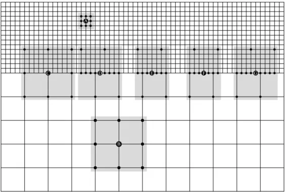
552 Figure 5. Nine-point Discontinuous-grid configurations for N=5.

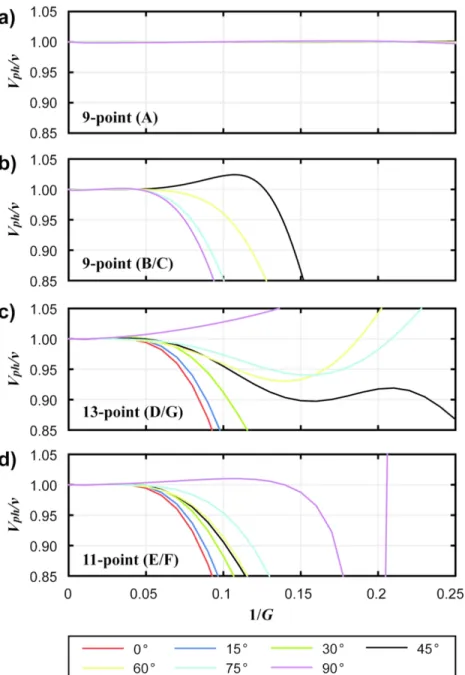
553 Figure 6. Normalized phase velocity curves for different FDFD operators in Figure 5,

554 with standard nine-point operators at gridpoints (a) A and (b) B/C, (c) 13-point

4 5 6 7 8 9 10 11 12 13 14 15 16 17 18 19 20 21 22 23 24 25 26 27 28 29 30 31 32 33 34 35 36 37 38 39 40 41 42 43 44 45 46 47 48 49 50 51 52 53 54 55 56 57 58 59

(25)

For Peer Review

555 operator at gridpoint D/G, and (d) 11-point operator at gridpoint E/F, respectively.

556 Figure 7. A velocity model discretized using (a) uniform-grid, (c) N=3

557 discontinuous-grid, and (e) N=5 discontinuous-grid. The corresponding impedance

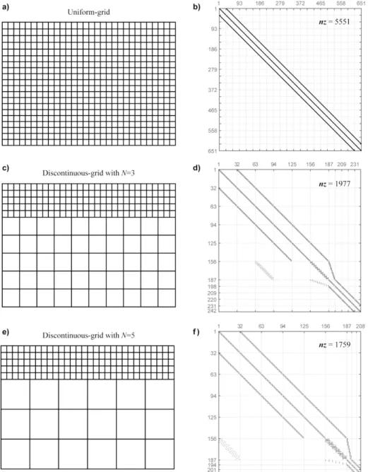
558 matrices are shown in (b), (d) and (f), respectively. Gray areas are nonzero elements,

559 with their numbers denoted by nz.

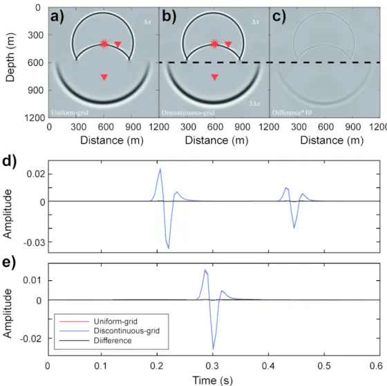
560 Figure 8. Comparison between the uniform- and discontinuous-grid schemes with

561 N=3. Shown in (a) and (b) are wavefield snapshots at 0.4 s calculated using uniform

562 and discontinuous grids. Shown in (c) is the differential wavefield amplified by 10x.

563 The dashed line in (b) denotes the boundary between differently-gridded areas. The

564 source is denoted by a red star. (d) and (e) are synthetic seismograms at two receivers

565 at (750, 400) m and (600, 750) m (shown as reversed triangles in (a) and (b)). The red

566 and blue traces are from the uniform- and discontinuous-grid schemes respectively,

567 and black traces are their differences.

568 Figure 9. Similar to Figure 8 except the source is located in the high-speed layer at

569 (600, 675) m.

570 Figure 10. Comparison between the uniform- and discontinuous-grid schemes with

571 N=5. Similar to those in Figure 8, except the model velocity in the bottom layer is 5

572 times of that in the top layer.

573 Figure 11. Simulation results in a complex velocity model using both uniform- and

574 discontinuous-grid schemes. (a) The velocity model used in the simulation. (b) The

575 velocity versus depth at x=0 and 1903 m. (c) and (d) Wavefield snapshots at t=1 s

576 from uniform- and discontinuous-schemes, where dashed lines in (d) denoting

4 5 6 7 8 9 10 11 12 13 14 15 16 17 18 19 20 21 22 23 24 25 26 27 28 29 30 31 32 33 34 35 36 37 38 39 40 41 42 43 44 45 46 47 48 49 50 51 52 53 54 55 56 57 58 59

(26)

For Peer Review

577 boundaries between differently- gridded areas. (e) Differential wavefield (amplified

578 by 10x) between (c) and (d). (h)-(i) Synthetic seismograms calculated at locations

579 (550, 100) m, (1,268, 802) m, (954, 1,038) m and (634, 1,120) m. The red and blue

580 traces are from uniform- and discontinuous-grid schemes, and the black traces are

581 differential waveforms.

582 583

584 Table Captions

585 Table 1. Coefficients of different FDFD operators in Figure 1.

586 Table 2. Coefficients of different FD operators for discontinuous-grid scheme with

587 N=3.

588 Table 3. Coefficients of different FD operators for discontinuous-grid scheme with

589 N=5. 590 4 5 6 7 8 9 10 11 12 13 14 15 16 17 18 19 20 21 22 23 24 25 26 27 28 29 30 31 32 33 34 35 36 37 38 39 40 41 42 43 44 45 46 47 48 49 50 51 52 53 54 55 56 57 58 59

(27)

For Peer Review

Figure 1. Schematic of 2D FDFD schemes, where (a) is the general stencil, and (b) and (c) are two sample stencils. The locations circled by the red line are included in the summation.

155x105mm (300 x 300 DPI) 4 5 6 7 8 9 10 11 12 13 14 15 16 17 18 19 20 21 22 23 24 25 26 27 28 29 30 31 32 33 34 35 36 37 38 39 40 41 42 43 44 45 46 47 48 49 50 51 52 53 54 55 56 57 58 59

(28)

For Peer Review

Figure 2. Comparison of three sample FDFD stencils. Three rows from top to bottom (a) - (c) are for different cases, where geometries of stencils, dispersion curves, structures of impedance matrixes and synthetic snapshots are presented. Dispersion curves of different colors denote different propagation angles.

The calculation of the impedance matrix is based on a small 8×8 grid model. The simulation is based on the same 2D homogenous medium with a velocity of 3500 m/s, and a 30 Hz Ricker wavelet is used as the source. The spatial interval is 4 m for schemes in (a) and (b), but 2 m for scheme in (c), because of its

lower accuracy. 176x169mm (300 x 300 DPI) 4 5 6 7 8 9 10 11 12 13 14 15 16 17 18 19 20 21 22 23 24 25 26 27 28 29 30 31 32 33 34 35 36 37 38 39 40 41 42 43 44 45 46 47 48 49 50 51 52 53 54 55 56 57 58 59

(29)

For Peer Review

Figure 3. Nine-point discontinuous-grid configurations for N = 3. Gridpoints A and B are inside regular grids, while C, D and E are located in the fine-to-coarse connecting row where special stencils are used. Different

FDFD operators are designed based on the local distribution of surrounding points. D’ and E’ are distorted stencils used near the absorbing boundary.

129x97mm (300 x 300 DPI) 4 5 6 7 8 9 10 11 12 13 14 15 16 17 18 19 20 21 22 23 24 25 26 27 28 29 30 31 32 33 34 35 36 37 38 39 40 41 42 43 44 45 46 47 48 49 50 51 52 53 54 55 56 57 58 59

(30)

For Peer Review

Figure 4. Normalized phase velocity curves for three types of FDFD operators in Figure 3, with standard nine-point operators at gridpoints (a) A and (b) B/C, and (c) new nine-point operator at gridpoint D/E,

respectively. 81x91mm (300 x 300 DPI) 4 5 6 7 8 9 10 11 12 13 14 15 16 17 18 19 20 21 22 23 24 25 26 27 28 29 30 31 32 33 34 35 36 37 38 39 40 41 42 43 44 45 46 47 48 49 50 51 52 53 54 55 56 57 58 59

(31)

For Peer Review

Figure 5. Nine-point Discontinuous-grid configurations for N=5. 169x112mm (300 x 300 DPI) 4 5 6 7 8 9 10 11 12 13 14 15 16 17 18 19 20 21 22 23 24 25 26 27 28 29 30 31 32 33 34 35 36 37 38 39 40 41 42 43 44 45 46 47 48 49 50 51 52 53 54 55 56 57 58 59

(32)

For Peer Review

Figure 6. Normalized phase velocity curves for different FDFD operators in Figure 5, with standard nine-point operators at gridpoints (a) A and (b) B/C, (c) 13-point operator at gridpoint D/G, and (d) 11-point operator

at gridpoint E/F, respectively. 81x117mm (300 x 300 DPI) 4 5 6 7 8 9 10 11 12 13 14 15 16 17 18 19 20 21 22 23 24 25 26 27 28 29 30 31 32 33 34 35 36 37 38 39 40 41 42 43 44 45 46 47 48 49 50 51 52 53 54 55 56 57 58 59

(33)

For Peer Review

Figure 7. A velocity model discretized using (a) uniform-grid, (c) N=3 discontinuous-grid, and (e) N=5 discontinuous-grid. The corresponding impedance matrices are shown in (b), (d) and (f), respectively. Gray

areas are nonzero elements, with their numbers denoted by nz. 163x213mm (300 x 300 DPI) 4 5 6 7 8 9 10 11 12 13 14 15 16 17 18 19 20 21 22 23 24 25 26 27 28 29 30 31 32 33 34 35 36 37 38 39 40 41 42 43 44 45 46 47 48 49 50 51 52 53 54 55 56 57 58 59

(34)

For Peer Review

Figure 8. Comparison between the uniform- and discontinuous-grid schemes with N=3. Shown in (a) and (b) are wavefield snapshots at 0.4 s calculated using uniform and discontinuous grids. Shown in (c) is the differential wavefield amplified by 10x. The dashed line in (b) denotes the boundary between differently-gridded areas. The source is denoted by a red star. (d) and (e) are synthetic seismograms at two receivers at (750, 400) m and (600, 750) m (shown as reversed triangles in (a) and (b)). The red and blue traces are

from the uniform- and discontinuous-grid schemes respectively, and black traces are their differences. 85x85mm (300 x 300 DPI) 4 5 6 7 8 9 10 11 12 13 14 15 16 17 18 19 20 21 22 23 24 25 26 27 28 29 30 31 32 33 34 35 36 37 38 39 40 41 42 43 44 45 46 47 48 49 50 51 52 53 54 55 56 57 58 59

(35)

For Peer Review

Figure 9. Similar to Figure 8 except the source is located in the high-speed layer at (600, 675) m. 85x85mm (300 x 300 DPI) 4 5 6 7 8 9 10 11 12 13 14 15 16 17 18 19 20 21 22 23 24 25 26 27 28 29 30 31 32 33 34 35 36 37 38 39 40 41 42 43 44 45 46 47 48 49 50 51 52 53 54 55 56 57 58 59

(36)

For Peer Review

Figure 10. Comparison between the uniform- and discontinuous-grid schemes with N=5. Similar to those in Figure 8, except the model velocity in the bottom layer is 5 times of that in the top layer.

85x87mm (300 x 300 DPI) 4 5 6 7 8 9 10 11 12 13 14 15 16 17 18 19 20 21 22 23 24 25 26 27 28 29 30 31 32 33 34 35 36 37 38 39 40 41 42 43 44 45 46 47 48 49 50 51 52 53 54 55 56 57 58 59

(37)

For Peer Review

Figure 11. Simulation results in a complex velocity model using both uniform- and discontinuous-grid schemes. (a) The velocity model used in the simulation. (b) The velocity versus depth at x=0 and 1903 m. (c) and (d) Wavefield snapshots at t=1 s from uniform- and discontinuous-schemes, where dashed lines in (d) denoting boundaries between differently- gridded areas. (e) Differential wavefield (amplified by 10x) between (c) and (d). (h)-(i) Synthetic seismograms calculated at locations (550, 100) m, (1,268, 802) m,

(954, 1,038) m and (634, 1,120) m. The red and blue traces are from uniform- and discontinuous-grid schemes, and the black traces are differential waveforms.

173x205mm (300 x 300 DPI) 4 5 6 7 8 9 10 11 12 13 14 15 16 17 18 19 20 21 22 23 24 25 26 27 28 29 30 31 32 33 34 35 36 37 38 39 40 41 42 43 44 45 46 47 48 49 50 51 52 53 54 55 56 57 58 59