全球商學院之排序與分群

全文

(1)國立交通大學資訊管理研究所碩士論文. 全球商學院之排序與分群 Ranking and Grouping on World Business Schools. 研究生：楊秉中指導教授：黎漢林. 中華民國九十三年. 教授. 六月.

(2) 全球商學院之排序與分群 Ranking and Grouping on World Business Schools. 研究生：楊秉中. Student：Ping-Chung Yang. 指導教授：黎漢林. Advisor：Han-Lin Li. 國立交通大學資訊管理研究所碩士論文. A Thesis Submitted to Institute of Information Management College of Management National Chiao Tung University in Partial Fulfillment of the Requirements for the Degree of Master of Business Administration in Information Management June 2004 Hsinchu, Taiwan, the Republic of China. 中華民國九十三年六月.

(3) 全球商學院之排序與分群. 學生：楊秉中. 指導教授：黎漢林教授. 國立交通大學資訊管理研究所碩士班. 摘. 要. 時下許多雜誌如 Time、U.S. News 和 Financial Times 等，利用不同數學公式出版全美或全球大學評鑑刊物，然而卻被許多人在評比方法之確切性及資料正確性上遭受批評。本論文所提出的方法能利用決策者所提供之偏好自行計算出各評比指標之權重，並以表格及 3D Ball 之視覺工具呈現排序與分群結果。以此結果為參考，決策者能再次加入偏好或是在決策單位﹝DMU﹞間作修正，以獲得想要之結果。此方法能根據決策者多次加入之偏好來計算與其邏輯相似之評比結果，以達成協助決策者做明確的決策選擇。. 關鍵字：排序、分群、商學院、階層分析法、偏好. i.

(4) Ranking and Grouping on World Business Schools Student：Ping-Chung Yang. Advisors：Dr. Han-Lin Li. Institute of Information Management National Chiao Tung University. ABSTRACT. Companies like Time, U.S. News, and Financial Times use different ranking models to publish university ranking guides. However, many critics say the ranking formulas are constantly changing and the data is highly manipulable. In the proposed model, the decision makers can rank universities based on their preferences. Based on the preferences, this model will automatically generate a set of weightings for criteria in the ranking process. The ranking and the grouping result will be displayed using both tables and 3D ball visualization tool. The decision makers can further specify the relationships between DMUs or add more preferences to obtain desired outcome. Providing decision makers various chances and means to add their opinions through out the ranking process, this model can ensure that the result are consistent with what decision makers had in mind and can ,hence, help them in the decision making process.. Keyword: Business School, Ranking, Grouping, Pairwise Comparison, AHP, Preference. ii.

(5) Acknowledgements First of all, I would like to thank my family, who has stood beside me and supported me all these years. My deepest thanks to Professor Li, your wisdom has inspired me not only in academic areas but also my everyday life. My appreciations also goes to Susan, Vickie, Clair, and the office ladies from the office of Management College, you have provided me countless helps in every aspect. Also, the working opportunities you gave me have supported me financially though my study. Thanks to all the people in the Operation Management Lab. Special thanks to Connie Ma and Jamie Liu, who worked closely with me through out the research process. Thank you, James, Roger, Nanze, Eugene, Adam, Grace, Leo, Frank, Ivan, HsioChu, Yoyo, Kit, Fion, and JianZhi, you have made my research life colorful. Thank you DBIS Lab and Multimedia Lab. You are my second favorite places to go. Days won’t pass smoothly if I miss visiting your lab for just one day. Thanks, Clay, Annie, Nancy, Edward, Fumi, Johnny, Jinny, Rita, Taxier, Mike, Christine, and JiaYuan. Amber, Sandy, and Vivienn, gossips with you girls were fun. Stan, Joyku, and Terry, it was fun playing various sports with you guys. You are also the source of my entertainments. Thank you all, accompanied me in the past two years. This thesis is dedicated to all of you who care about me. Hope you will enjoy it. Ping-Chung Yang June 24th 2004 OM Lab, NCTU, Hsinchu Taiwan. iii.

(6) Table of Contents Content............................................................................................................................i List of Tables..................................................................................................................v List of Figures ...............................................................................................................vi 1. Introduction...........................................................................................................1 1.1 Background ....................................................................................................1 1.2 Objective ........................................................................................................2 1.3 Organization of Study ....................................................................................3 1.4 Scope and limitations.....................................................................................3 2. Literature Review..................................................................................................1 2.1 Ranking Methodology ...................................................................................1 U.S. News and World Report.........................................................................1 Financial Times..............................................................................................2 2.2 Data Envelopment Analysis...........................................................................5 2.3 Analytic Hierarchy Process............................................................................7 2.4 Intransitivity.................................................................................................12 2.5 Clustering.....................................................................................................14 3. Ranking and Grouping Models...........................................................................17 3.1 Common Weight Model...............................................................................18 3.2 3D Spherical Model .....................................................................................23 3.3 Clustering.....................................................................................................30 4. Iterative Ranking and Grouping..........................................................................34 5. Conclusion ..........................................................................................................50 References....................................................................................................................51 Appendex .....................................................................................................................52 U.S. News and World Report 2005 Ranking .........................................................52 Financial Times 2004 Ranking ..............................................................................56. iv.

(7) List of Tables Table 2.1 Table 2.2 Table 2.3 Table 2.4 Table 2.5 Table 2.6 Table 2.7 Table 3.1 Table 3.2 Table 3.3 Table 3.4 Table 3.5 Table 3.6 Table 3.7 Table 3.8 Table 4.1 Table 4.2 Table 4.3 Table 4.4 Table 4.5 Table 4.6 Table 4.7 Table 4.8 Table 4.9. Hard data provided by John on cars..........................................................9 Comparison score for each car with respect to each criterion ................10 Normalized comparison table .................................................................10 Priority vectors with respect to each criterion ........................................11 Comparison tables and weightings for criteria ....................................... 11 Preference matrix on six nodes ...............................................................13 Preference Matrixes ................................................................................14 Variables for Common Weight Model ....................................................19 Normalized hard data from Financial Times’ 2004 Ranking ..................21 Results from Common-Weight Model ....................................................22 Variables and descriptions.......................................................................24 Coordinates for each universities ............................................................27 Dissimilarity matrix ................................................................................28 Variables and descriptions for Clustering Model ....................................30 Groupings for universities.......................................................................32 Hard data on five universities John selected ...........................................36 Variables for Model 1..............................................................................37 Tournament Matrix for Universities........................................................38 Reduced tournament matrix ....................................................................40 Results from initial run of the model ......................................................43 Grouping table for the initial result.........................................................43 New grouping table specified by John ....................................................45 Results form the groupings specified by John ........................................45 Results with preference ...........................................................................47. v.

(8) List of Figures Figure 2.1 Figure 3.1 Figure 3.2 Figure 3.3 Figure 4.1 Figure 4.2 Figure 4.3 Figure 4.4 Figure 4.5 Figure 4.6 Figure 4.7. Preference Graph of six nodes...............................................................13 Flowchart...............................................................................................17 3D ball with DMUs projected on the surface........................................29 Groupings for twenty universities .........................................................33 Flow chart for Iterative Ranking and Grouping Model.........................35 Preference graph from Table 4.3 ...........................................................39 New preference graph............................................................................40 Flowchart for preference addition .........................................................42 Initial grouping situation represented on 3D ball ..................................44 New coordinates and groupings for the universities .............................46 New coordinates for the university with John’s preference. .................48. vi.

(9) 1. Introduction. Background Every year, many high school graduates and university graduates purchase University Ranking Guides to help them select the right undergraduate program or graduate program that is best suited for them. Although among the quarter million freshmen who participated in the survey done by the Higher Education Research Institute, only 8.6% responded that the rankings were very important to them when selecting colleges or universities (Crissey, 1997). The reasons may lie on the question of ranking methodology. How do we know these rankings are right for the students and rank universities in the way the students needed? How do we know the criteria participated in the ranking system are what the ones students consider important? These are some of the key concerns which should be solved.. Currently, there are many publishers which release various kinds of ranking each year. US News and World Report, for example, started releasing university ranking in with the October issue in late 1980’s. They have realized that in the subsequent years, the October issue had sold many more copies than any other issues. Hence, they decided to start publishing an independent issue for university ranking. In the 1990’s, many other publishers like Time, Newsweek, Money Magazine, and many more have also realized that the market for university ranking is enormous and have started to create their own rankings and publish them. Similarly, Canada, Asia, and Europe all have magazines that do rankings for universities in different regions.. 1.

(10) Objective The ranking guides currently in the market are heavily criticized by many people ranging from educational field to people in the publishing industry. Some of these criticisms are as follow: (1) To increase the sales, publishers may introduce new measures or change the weightings of measures from year to the next (Gater, 2003). (2) Some of the factors are highly manipulable, and, as a result, the ranking outcome is meaningless (Leiter, 2003). (3) Ranking formula and factors participated in the ranking process are constantly changing, so the results are high in variation (Levin, 1997).. In this study, we propose a new ranking method that can help the Decision Makers (DM) rank Decision Making Units (DMUs). The characteristics are listed below: (1) The model can automatically generate weightings with minimal human influence. (2) Ranking can still be done with minimum information from Decision Makers, i.e. preferences. (3) 3D ball representation gives clear view on the correlations. (4) This model allows DM to add preferences through out the ranking process. (5) DM can specify groupings for DMUs.. 2.

(11) Organization of Study Chapter 2 reviews related literatures. The discussed area will include review on current ranking methods, Data Envelopment Analysis, Analytic Hierarchy Process, Transitivity, and Clustering.. Chapter 3 explains the whole ranking and grouping model by using a small data set. The concept of each mathematical model used in the ranking and grouping process will be explained in detail.. Chapter 4 ranks schools using the hard data from Financial Times using the new model and compare with the original ranking.. Conclusion drawn from the experiment and discussions will be presented in chapter 5, along with the recommendations for future works.. Scope and limitations This study will focus on the mathematical model, which will try to generate a set of optimal weightings without the needs of Decision Makers to specify the weightings manually .. 3.

(12) 2. Literature Review 2.1. Ranking Methodology There are several rankings published in the market. Each of them has different. methodology to rank universities. They vary in criteria selection, assignment of weightings, and raw data, just to name a few. Let us look at few of the more popular ranking systems and their methodology.. U.S. News and World Report Source: www.usnews.com U.S. News ranks business colleges in United States in 2004 and listed 82 of them. They have used three major sections with total of eight criteria for the entire ranking process. These criteria are listed below with their weightings and descriptions. (1). Quality Assessment (total 40%): I. Peer Assessment (25%) – Deans and directors from business schools of accredited programs were asked to rate programs from marginal (1) to outstanding (5). Notice that 56% of them have returned the survey. II. Recruiter Assessment (15%) – Corporate recruiters were also asked to rank the programs which they have hired employee from in the previous year. However, only 32% of them replied the survey.. (2). Placement Success (total 35%): I. Average Starting Salary and Bonus (14%) – This is the mean of starting salary and bonus. 1.

(13) II.. Percentage of Graduates Employed at Graduation (7%) – The percentage of emplacement rate is measure before the students actually graduate from full-time MBA program. III. Percentage of Graduates Employed 3 Months after Grad (14%) – The percentage of employed graduates three months after completing the full-time MBA program.. (3). Student Selectivity (total 25%): I. Average Undergrad GPA (7.5%) – The average GPA of new students. II. Average GMAT (16.25%) – Average GMAT score of new students who are accepted to the full-time MBA program. III. Acceptance Rate (1.25%) – Percentage of accepted applications.. From their hard data, we have tried to duplicate their ranking formula and have found a very similar ranking result with identical overall scores. The formula n ⎛ Ck − Ck ⎞ ⎟ where n is the total number should be very close to Score = ∑ ⎜ wk * ⎟ ⎜ C C − k =1 ⎝ k k ⎠. of criteria and Ck is the value of kth criterion and Ck and Ck are the maximum and minimum values of kth criteria.. Financial Times Source: www.ft.com Unlike U.S. News & World Report, Financial Times (FT) has ranked business schools from all over the world and has listed 100 of them. FT has also selected twenty criteria for the ranking process. The following are those criteria and their weightings.. 2.

(14) (1). Weighted Salary (20%) – This is the average salary today with adjustment for different industries. Also, this figure is the average salary three years after graduation. (in US dollars). (2). Salary Percentage Increase (20%) – The percentage increase in salary from beginning of MBA program to three years after graduation.. (3). Value for Money (3%) – This is calculated by the salary earned by MBA graduates three years after graduation with the course costs and the opportunity cost, while still in school and not employed.. (4). Career Progress (3%) – The degree to which alumni have moved up the career ladder three years after graduating. Progression is measured through changes in level of seniority and the size of company in which they are employed.. (5). Aims Achieved (3%) – The extent ot which alumni fulfilled their goals or reasons for doing an MBA. This is measured as a percentage of total returns for a school and presented as a rank.. (6). Placement Success (2%) – The percentage of 2000 alumni that gained employment with the help of career advice. The data is presented as rank.. (7). Alumni Recommendation (2%) – Alumni of 2000 were asked to name three business schools from which they would recruit MBA graduates. The figure represents the number of votes received by each school. The data is presented as a rank.. (8). International Mobility (6%) – A rating system that measures the degree of international mobility based on the employment movements of alumni between graduation and today.. (9). Employed at Three Months (2%) – the percentage of the most recent graduating class that had gained employment within three months.. (10) Women Faculty (2%) – Percentage of female faculty. 3.

(15) (11) Women Students (2%) – Percentage of female students. (12) Women Board (1%) – Percentage of female members in the advisory board. (13) International faculty (4%) – The percentage of international students. (14) International Students (4%) – Percentage of the board whose nationality differs from their country of employment. (15) International board (2%) – Percentage of the board whose nationality differs from their country of employment. (16) International Experience (2%) – Weighted average of three criteria that measure international exposure during the course. (17) Languages (2%) – Number of additional languages required on completion of the MBA. Where a proportion of students required another language due to an additional diploma or degree chosen that figure is included in the calculations but not presented in the final table. (18) Faculty with Doctorates (5%) – Percentage of faculty with a doctoral degree. (19) FT Doctoral Rating (5%) – Number of doctoral graduates from the last three academic years with additional weighting for those graduates taking up a faculty position at one of the top 50 school in this year’s ranking. (20) FT Research Rating (10%) – a rating of faculty publications in 40 international academic and practitioner journals. Points are accrued by the business school at which the author is presently employed. Adjustment is made for faculty size.. The results and hard data of both U.S. News and World Report and Financial 4.

(16) Times are attached in the Appendix section. Both publishers have worked with other companies for data collection. However, they did not explain how the weightings for the criteria were decided. Moreover, perhaps because U.S. News and World Report is the most recognized publisher in university ranking, it receives many criticisms on both the changes on weightings from year to year and the correctness of hard data. On the contrary, Financial Times has fixed their weightings. However the way hard data is presented has been modified from year to year. For example, the criterion “value for money” was a score ranging from 1 to 5 in year 2002 and 2003 ranking. In 2004, this criterion has been changed into “value for money rank”. When it was a score from 1 to 5, there can be only 50 different scores and is unlikely that all the variation of the score will be assigned. Hence there are many schools with the same scores. When it changed to rank, only few schools are being ranked as the same, so the variation is larger. This problem arises on more than one criterion in Financial Times’ ranking.. 2.2. Data Envelopment Analysis Data Envelopment Analysis (DEA) is a method for evaluating the activity. performance, especially for organizations such as business firms, government agencies, hospitals, educational institutions, and etc (Cooper etc. 1999). A commonly used measure for efficiency is the output-input ratio. Number of items sold in a store will be an example of the output; number of sales clerk in the store will be the input. Hence, the efficiency of this store, basing on only these two criteria, will simply be NumberOfGoodsSold / NumberOfClerk. These comparable entities are often called Decision Making Units (DMUs).. 5.

(17) The purpose of DEA is to empirically estimate the efficient frontier based on the set of available DMUs and assumes that each performance measure can be categorized as either an input or an output (Schrage, 1997). It provides the user information about both efficient and inefficient units along with the efficiency scores and reference sets for inefficient units (Halme etc, 1999). An Efficient Frontier is a line that has at least one DMU point touching it. The DMUs, who touch the EF line, are the most efficient DMUs. The idea of Production Frontier is first discussed by Farrell in 1975 which has three assumptions. The attractive feature of DEA is that it produces efficiency score between 0 and 1.. In 1978, Charnes, Cooper, and Rhodes proposed a DEA model called the CCR model basing on Farrell’s single input-output model in 1975. CCR model is designed to measure the cases of multi input and multi output. The following is the pseudo-code for the CCR model. Ur represents the weighting for rth output criterion and Vi represents the weighting for ith input criterion. They are automatically generated when the score of kth DMU is maximized. Yr and Xi are the output and input criteria. For each DMU k s. MAX Score k =. ∑U Y. r. ∑V X. i. r. r =1 m i =1. such that Score k ≤ 1 Ur > 0 Vi > 0 6. i.

(18) Where Yr is the rth output of DMU Xi is the ith input of DMU Ur is the weighting for rth output Vi is the weighting for ith input. In this CCR model, it will calculate the score of each DMU based on the weightings that can maximize the score of current DMU, which means that the nth DMU can obtain the best score with nth set of weightings. Hence, if there are n numbers of DMUs, then there will have n set of weightings. kth set of weighting is determined under the condition that they can maximize the Scorek. All the scores have to be between 0 and 1. Once score of each DMU is determined, it then compares all of them again with their score. The DMU with highest score is the most efficient one.. 2.3. Analytic Hierarchy Process The Analytical Hierarchy Process (AHP) was proposed by Saaty in 1980 and his. collaborators as a method for establishing priorities in multi-criteria decision making contexts based on variables that do not have exact numerical consequences (Genest, 1996). It also helps people set priorities and make the best decision when both qualitative and quantitative aspects of a decision need to be considered. AHP not only helps decision makers arrive at the best decision, but also provides a clear rationale that it is the best.. 7.

(19) AHP can be conducted in three steps: Setp 1:. Perform pairwise comparisons between each DMU on every criterion In this step, the goal is to obtain the priorities between DMUs for each criterion. To do so, a pairwise comparison has to take place between each DMU with respect to each criterion. For each criterion, a m by m matrix, where m is the number of DMUs, will be generated and the priority vector will be calculated from this matrix. Priority vector displays the preference orders for each DMU with respect to criteria. Since there are n numbers of criteria, n number of priority vector will be generated at the end.. Step 2:. Perform pairwise comparison between each criterion In the decision making process, not every criterion is quantitatively measurable, so a pairwise comparison between each criterion has to take place in order to specify the importance between each criterion. From the comparison, a set of weightings can be found for score calculation at the last step.. Step 3:. Compute final scores for DMUs With the priority vectors and the weightings for criteria, DM can now calculate the score for each DMU. DMU with the higher score should be the better alternative for the Decision Maker.. Following is an illustration of an example of a student, John, wanting to purchase a car. Due to his financial limitation, John can only buy a second hand car, and only. 8.

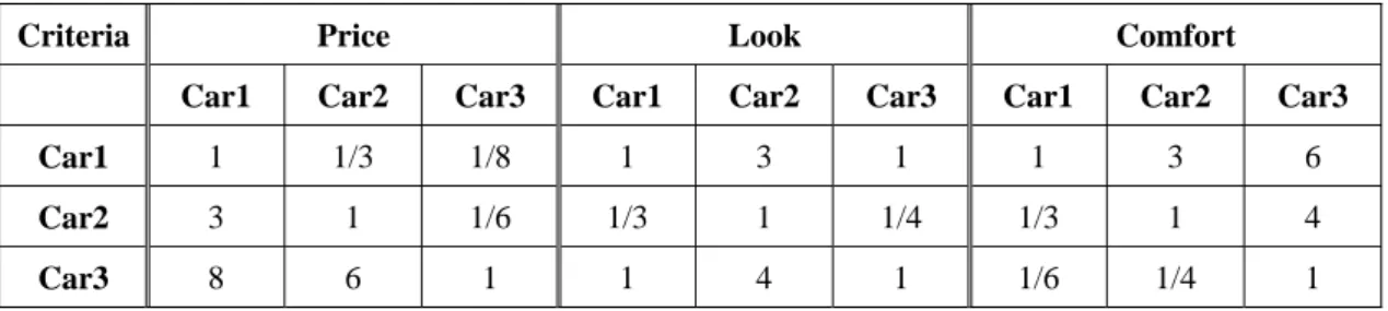
(20) has few things that he really car. He wants to buy a car that is cheap, nice out look, and comfortable. However, among the three cars he has in mind, none of them has best score on each of these criteria. He has decided to use AHP to help him select a car from these three. Table 2.1 lists all the data he gathered about these three cars.. Table 2.1. Hard data provided by John on cars. Price. Look. Comfort. Car 1. 13100. Good. Very good. Car 2. 12000. Fair. Good. Car 3. 9800. Good. Fair. To perform pairwise comparison between each car with respect to each criterion, a priority score has to be assigned to each comparison. The scores can range from 1 to 9, where 9 is the most satisfactory score. Notice that if a DM compare A1 to A2 and assigns a score of 4, then the score between comparison of A2 and A1 will be the inverse of A1 and A2’s, which will be 1/4. This property can ensure the logical consistency for each comparison.. 1 Choice i and j are equally important 3 Choice i is weakly more important than j 5 Choice i is strongly more important than j 7 Choice i is very strongly more important than j 9 Choice i is absolutely more important than j 2, 4, 6, 8 are intermediate values. After finishing pairwise comparisons, matrixes with these priority scores will be generated (Table 2.2).. 9.

(21) Table 2.2. Comparison score for each car with respect to each criterion. Criteria. Price. Look. Comfort. Car1. Car2. Car3. Car1. Car2. Car3. Car1. Car2. Car3. Car1. 1. 1/3. 1/8. 1. 3. 1. 1. 3. 6. Car2. 3. 1. 1/6. 1/3. 1. 1/4. 1/3. 1. 4. Car3. 8. 6. 1. 1. 4. 1. 1/6. 1/4. 1. From these matrixes, normalization has to be done before the priority vectors can be calculated (Table 2.3). Normalization is simply divides each value by the sum of corresponding column. For example, the normalized value between car2 and car3 with respect to price is calculated by (1/6) / (1/8 + 1/6+ 1) = 0.1290.. Table 2.3. Normalized comparison table. Criteria. Price. Look. Comfort. Car1. Car2. Car3. Car1. Car2. Car3. Car1. Car2. Car3. Car1. 0.0833. 0.0454. 0.0967. 0.4286. 0.375. 0.4444. 0.6666. 0.7059. 0.5454. Car2. 0.250. 0.1363. 0.1290. 0.1428. 0.125. 0.1111. 0.2222. 0.2352. 0.3636. Car3. 0.6666. 0.8182. 0.7742. 0.4286. 0.5. 0.4444. 0.1111. 0.0588. 0.0909. Each criterion has its own priority vector and the values in the vector can be seen as the score of each DMU on corresponding criterion. The values in the priority vectors are the sum of rows from the normalized pairwise comparison matrix and divided by the number of DMUs, as in Table 2.4. The values in priority vector for price is calculated as follow: (0.0833 + 0.0454 + 0.0976) / 3 = 0.2254 (0.2500 + 0.1363 + 0.1290) / 3 = 0.5153 (0.6666 + 0.8182 + 0.7742) / 3 = 2.2590. 10.

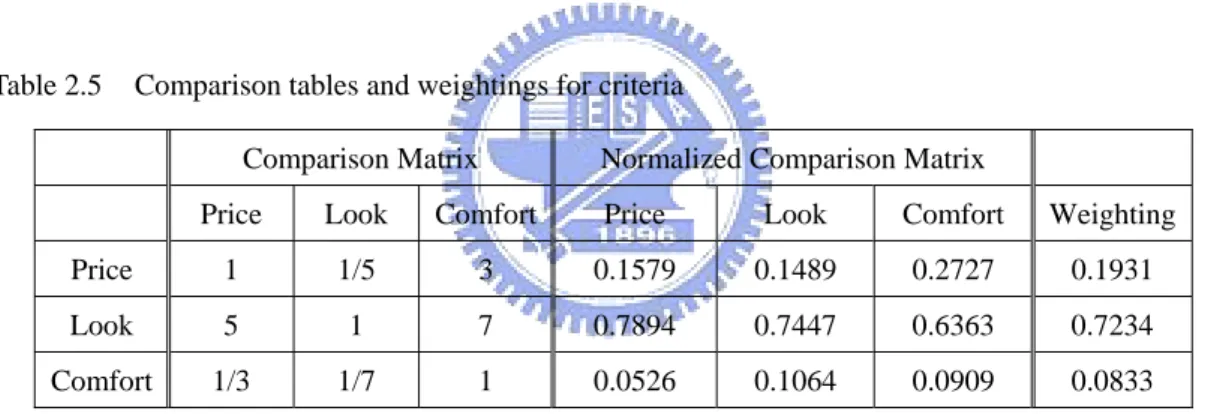
(22) Table 2.4. Priority vectors with respect to each criterion Priority Vector for Price. Priority Vector for Look. Priority Vector for Comfort. Car1. 0.0751. 0.4160. 0.6393. Car2. 0.1717. 0.1263. 0.2736. Car3. 0.7530. 0.4576. 0.0869. After the values of priority vector is calculated, pairwise comparison has to perform on criteria to obtain the weightings for each criterion. Similar to previous steps, a 3 by 3 matrix, with criteria on both row and column, will be created. Using the same calculation method for priority vector, the weighting for each criterion can also be found (Table 2.5).. Table 2.5. Comparison tables and weightings for criteria Comparison Matrix. Normalized Comparison Matrix. Price. Look. Comfort. Price. Look. Comfort. Weighting. Price. 1. 1/5. 3. 0.1579. 0.1489. 0.2727. 0.1931. Look. 5. 1. 7. 0.7894. 0.7447. 0.6363. 0.7234. Comfort. 1/3. 1/7. 1. 0.0526. 0.1064. 0.0909. 0.0833. The weightings on Table 2.5 suggest that Look is the most important criterion for John. Price is the next concern and comfort is the last. With the weightings on the criteria and the priority vectors on each criterion, the score for each car can now be calculated as follow:. Car 1: (0.0751 * 0.1931)+(0.4160 * 0.7234)+(0.6393 * 0.0833) = 0.3687 Car 2: (0.1717 * 0.1931)+(0.1263 * 0.7234)+(0.2736 * 0.0833) = 0.1473 Car 3: (0.7530 * 0.1931)+(0.4576 * 0.7234)+(0.0896 * 0.0833) = 0.4839. 11.

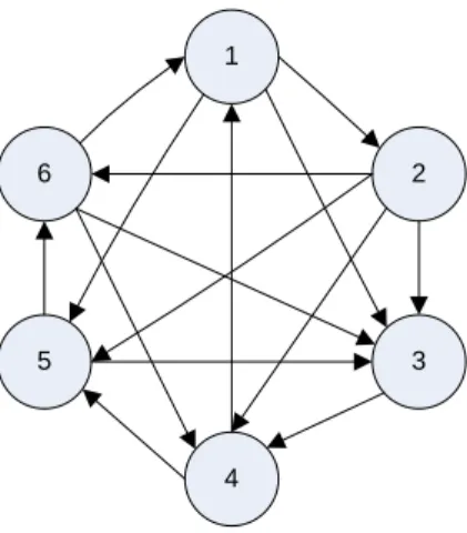
(23) From the calculation, Car 3 has the highest score and should be the best choice for John to consider.. 2.4. Intransitivity When Decision Makers are making decisions, some do a pairwise comparison. with AHP before they make the actual decision. However, AHP does not have a means for detecting an intransitivity situation. An intransitivity is when A > B, B > C, but C > A. This situation is also called logically inconsistent. When there is a cycle exists in the decision process and is not very logical. Hence, the intransitivity detection is a very important process before the any decision is made.. In Gass’ study (1998), he presented a way to detect the intransitivity with simple matrix operation. Theorem: Let P be the preference matrix of a preference diagram D. Then in Pk, the (i,j) entry, denoted by Pi,j(k) , is the number of sequences in D of length k from node vi to node vj. (Pk is the kth power of P). The theorem states that Pi,jk denotes the number of cycles, with different sequence. Take a preference graph shown in Figure 2.1 as an example. We can generate a tournament matrix from this preference graph. The preference matrix P, Table 2.11, has values of 0 or 1. Pi,j is set to 1 if i is smaller than j.. 12.

(24) Table 2.6 Preference matrix on six nodes. 1. 6. P1. P2. P3. P4. P5. P6. P1. 0. 0. 0. 1. 0. 1. P2. 1. 0. 0. 0. 0. 0. P3. 1. 1. 0. 0. 1. 1. P4. 0. 1. 1. 0. 0. 1. P5. 1. 1. 0. 1. 0. 0. P6. 0. 1. 0. 0. 1. 0. 2. 5. 3. 4. Figure 2.1 Preference Graph of six nodes. From this preference matrix, we can apply the theorem to this matrix and look for the cycles. Since the theorem said that the value of Pijk means there are the same numbers of combinations of sequences in the preference graph of length k from node i to node j. Similarly, if we look at Piik, then this will mean the sequence start at node i and come back to node i with the length of k. Hence, we can simply check the diagonal of each Pk for k = 3 up to k = n, where n is the number of nodes.. Table 2.7a to Table 2.7d are the power of preference matrix from P3 to P6. In Table 2.7a, we can see that the diagonal has nonzero values. P113 is 4, so there are four cycles with the length of 3 and the starting and ending node is P1. The cycles are (P1, P2, P4, P1), (P1, P3, P4, P1), (P1, P2, P6, P1), and (P1, P5, P6, P1). With the same technique, it is very easy to find the existence of cycles for any given preference graph. From Table 2.7b to Table 2.7d, it is clear that there are cycles with the length of 4, 5, and 6.. 13.

(25) Table 2.7 Preference Matrixes (a). P3 of Preference Matrix. (b). P1. P2. P3. P4. P5. P6. P1. 4. 3. 0. 1. 2. 1. P2. 0. 2. 1. 0. 1. P3. 3. 4. 2. 3. P4. 4. 3. 0. P5. 2. 4. P6. 1. 1. (c). P5 of Preference Matrix. P1. P2. P3. P4. P5. P6. P1. 5. 4. 1. 6. 1. 5. 1. P2. 4. 3. 0. 1. 2. 1. 1. 4. P3. 7. 10. 3. 4. 6. 8. 4. 1. 2. P4. 4. 7. 4. 5. 2. 8. 1. 1. 3. 3. P5. 8. 8. 1. 5. 4. 4. 1. 2. 0. 3. P6. 2. 6. 2. 1. 4. 4. (d). P6 of Preference Matrix. P1. P2. P3. P4. P5. P6. P1. 6. 13. 6. 6. 6. 12. P2. 5. 4. 1. 6. 1. P3. 19. 21. 4. 13. P4. 13. 19. 5. P5. 13. 14. P6. 12. 11. 2.5. P4 of Preference Matrix. P1. P2. P3. P4. P5. P6. P1. 25. 30. 6. 12. 18. 18. 5. P2. 6. 13. 6. 6. 6. 12. 11. 14. P3. 36. 42. 13. 30. 18. 36. 6. 12. 13. P4. 36. 36. 6. 25. 18. 24. 5. 12. 5. 14. P5. 24. 36. 12. 18. 19. 30. 1. 6. 6. 5. P6. 18. 18. 6. 18. 6. 19. Clustering Clustering involves dividing a set of data points into non-overlapping into groups,. where points in each group are more similar to each other than to points in other groups (Faber, 1994). When a set of data is clustered, every point is assigned to a group and every group can be characterized by a single reference point, normally the average of points in the same group.. 14.

(26) There are several techniques in the field of clustering. General clustering techniques are Hierarchical clustering, K-Mean clustering, Incremental clustering, and Probability-based clustering. K-mean clustering is also called Iterative Distance-based clustering. The character “k” in the name of K-mean is the number of groups, or clusters, DM wants to make. The basic idea for K-mean is randomly start with k number of points and assign each data point to one of the reference point in k by calculating the minimal total distance. Once the groups are determined, it then tries to adjust the position of the reference points so that it will locate in the center of corresponding group. The algorithm for the k-mean clustering is shown below.. Algorithm for K-mean Clustering: (1) Choose k centroid points. (2) Calculate the distance of each point to all centroids. (3) Get the minimum distance. This data is said belong to the cluster that has minimum distance from this data (4) Adjust the centroid location based on the current data updated data. (5) Assign all the data to this new centroid. (6) Repeat until no data is moving to another cluster anymore.. 15.

(27) In this study, the proposed model will be able to generate a set of weightings for criteria based on the preferences given by the decision makers. The model has applied similar idea from Data Envelopment Analysis. In DEA, it is trying to measure the efficiency based on maximizing the score of DMU. However, in the proposed model, it will try to maximize the rank for each DMU instead of score. The concept from Analytic Hierarchy Process is also used to create tournament matrix for ranking by doing pairwise comparison. Gass’ technique is also used to ensure the non-existence of intransitivity. Last but not least, the concept from K-mean clustering will be modified to help this ranking method to present the data points on a 3D ball to help DM make decisions.. 16.

(28) 3. Ranking and Grouping Models In this chapter, the ranking and grouping process can be break down into two major parts. First part will deal with the actual ranking and score calculation. The second part is mapping each school onto a 3D ball and clustering these data points. Figure 3.1 shows the entire process of proposed ranking and grouping model.. Figure 3.1 Flowchart. 17.

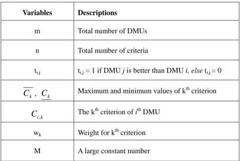
(29) 3.1. Common Weight Model. As discussed in chapter 2, DEA is mainly used for efficiency measurement. The concept of DEA is to calculate the ratio between inputs and outputs, and rank each DMU (Data Making Unit) by their maximized scores. In this ranking objective, however, DEA is not the perfect tool for the ranking process because the most efficient DMU might not be the best choice for DM (Decision Maker). Moreover, , sometimes criteria are hard to distinguish from input or output, the proposed method has modified the traditional DEA method to meet the DMs’ requirement without the need to identify inputs and outputs for criteria. This model will automatically ranks and groups the DMUs based on the absolute dominance relationships found in the hard data, so the DMs do not need to worry about assigning weightings for each criterion. This is a big improvement from the traditional ranking systems, which often have controversy on weighting settings.. In the experiments, Lingo8.0 is used as the optimization tool. Given the correct model and inputs, the system will calculate the ideal weights for each criterion, which will allow us to rank the DMUs and map each DMU to a coordinate on 3D ball to help DM visualize the relationships between DMUs, as well as the correlation between DMUs. In this section, the mathematical model and the concept behind it will be discussed in detail and the model will be applied on an example of 20 universities. Before the mathematical model is being discussed, Table 3.1 lists and describes the variables, following is the model.. 18.

(30) Table 3.1. Variables for Common Weight Model. Variables. Descriptions. m. Total number of DMUs. n. Total number of criteria. ti,j. ti,j = 1 if DMU j is better than DMU i, else ti,j = 0. Ck , Ck. Maximum and minimum values of kth criterion The kth criterion of ith DMU. C i ,k wk. Weight for kth criterion. M. A large constant number. Common Weight Model (Model 1): m. m. ∑∑. Min. i =1 j ≠ i. (3.1). ti, j. Subject to ⎛. ∑ ⎜⎜⎜ w n. k =1. k. ⎝. ⎛ C i,k − C k ∗⎜ ⎜ C −C k ⎝ k. n. ∑w k =1. k. =. wk ≥ ε ,. ⎞⎞ ⎟ ⎟ + (M ∗ t ) i, j ⎟ ⎟⎟ ⎠⎠. ≥. ⎛. ∑ ⎜⎜⎜ w n. k =1. ⎝. k. ⎛ C j ,k − C k ∗⎜ ⎜ C −C k ⎝ k. ⎞⎞ ⎟⎟ ⋅ ⎟ ⎟⎟ ⎠⎠. ∀ i, j and j ≠ i. (3.2). 1. (3.3). ∀ k. (3.4). t i , j ∈ {0,1}. (3.5). t i , j + t j ,i ≤ 1, ∀ i, j < i. (3.6). In this model, Lingo will generate a set of weightings for the ranking process. This model ranks the DMUs without DMs worrying about the numbers (weightings). Moreover, these weightings could be more convincing for some DM because these 19.

(31) numbers are generated by the system automatically based only on the absolute dominance relationships.. After this model is run by Lingo, Lingo will return a matrix with the size of m by m. This matrix will consist values of only 0 and 1. For tij, if tj > ti, then tij will be set to 1. The sum of each row will represent their rank correspondingly. The objective function (3.1) is trying to maximize the rank of each DMU by minimizing the sum of t for each row. Note that the DMU with lower the sum of t, the higher rank it will get.. ⎛ ⎜w ∑ ⎜ k k =1 ⎝ n. Constraint 3.2 is for determining the values of ti,j. If. ⎛ than ∑ ⎜ wk ⎜ k =1 ⎝ n. ⎛ C j ,k − C k ∗⎜ ⎜ Ck − Ck ⎝. ⎞⎞ ⎟ ⎟ is greater ⎟⎟ ⎠⎠. ⎞⎞ ⎟ ⎟ , then ti,j will be 0, since we are minimizing the sum of ti,j. ⎟⎟ ⎠⎠. ⎛ ⎜w ∑ ⎜ k k =1 ⎝ n. On the other hand, if. ⎛ C i ,k − C k ∗⎜ ⎜ Ck − Ck ⎝. ⎛ Ci ,k − C k ∗⎜ ⎜ Ck − Ck ⎝. ⎞⎞ ⎟ ⎟ is smaller than ⎟⎟ ⎠⎠. ⎛ ⎜w ∑ ⎜ k k =1 ⎝ n. ⎛ C j ,k − C k ∗⎜ ⎜ Ck − Ck ⎝. ⎞⎞ ⎟⎟ , ⎟⎟ ⎠⎠. in order to satisfy constraint 3.2, the value of M ∗ t i , j must not be 0, so ti,j will be set to 1.. Constraint 3.3 is to make sure that the sum of weights of all the criteria will be equal to 1. Also, constraint 3.4 ensures that the weights are all non-zero, so every criterion will be taken into account in this ranking process. Constraint 3.5 specifies that ti,j is a binary variable, which can only be 0 or 1. The last constraint is to insure that if i is better than j, then j can not be better than i at the same time.. Once the weights for each criterion are automatically generated by the model, score of each DMU will be calculated by equation 3.7 for future ranking purposes.. 20.

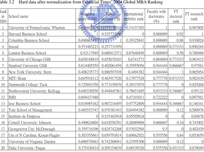
(32) This score function ensures that the scores are all between 0 and 1 by normalizing the hard data. This will help DM to see the differences in the scores.. (. ). n ⎛ Ci ,k − C k ⎞ ⎟ SCORE i = ∑ ⎜ wk ∗ ⎜ (C k − C k ) ⎟⎠ k =1 ⎝. (3.7). Table 3.2 shows the original hard data of the first twenty universities listed on the Financial Times’ 2004 Global MBA Ranking. The data has been normalized so that 1 is the maximum score and 0 is the minimum score. Notice that we have only chosen six criteria that have the heaviest weightings.. Table 3.2 Hard data after normalization from Financial Times’ 2004 Global MBA Ranking Rank in School name 2004 1. University of Pennsylvania: Wharton. 2. Harvard Business School. Weighted salary (US$). Salary International increase (%) mobility rank. Faculty with FT FT research doctorates doctoral rank (%) rank. 0.836865335 0.855670103. 0.74157303. 1. 1. 0.987805. 1 0.525773196. 0. 0.888889. 0.92. 1. 0.888889. 0.88. 0.939024. 0.888889 0.373333. 0.890244. 3. Columbia Business School. 0.696863457. 1. 0.39325843. 4. Insead. 0.553465223 0.257731959. 1. 4. London Business School. 0.42117949 0.680412371. 0.87640449. 0.56. 0.780488. 4. University of Chicago GSB. 0.658188819 0.855670103. 0.6741573. 0.888889. 0.888889 0.773333. 0.963415. 7. Stanford University GSB. 0.814405559 0.402061856. 0.35955056. 0.944444 0.866667. 0.97561. 8. New York University: Stern. 0.408235773 0.886597938. 0.4494382. 1. 0.865854. 9. MIT: Sloan. 0.645918112 0.463917526. 0.17977528. 0.777778 0.973333. 0.902439. 0.944444. 10 Dartmouth College: Tuck. 0.725693358 0.773195876. 0.30337079. 0.777778. 0. 0.829268. 11 Northwestern University: Kellogg. 0.640330558 0.494845361. 0.78651685. 0.833333 0.746667. 0.95122. 12 IMD. 0.694437488. 0. 0.47191011. 0.722222. 0. 0.097561. 13 Iese Business School. 0.018985162 0.907216495. 0.97752809. 0.944444 0.346667. 0.146341. 13 Yale School of Management. 0.485553747 0.979381443. 0.04494382. 0.888889. 0.12. 0.560976. 0 0.515463918. 0.95505618. 0. 0. 0.04878. 16 Cornell University: Johnson. 0.490624804 0.618556701. 0.28089888. 0.666667. 0.16. 0.743902. 17 Georgetown Uni: McDonough. 0.359716396 0.824742268. 0.53932584. 0.5. 0. 0.402439. 17 Uni of N Carolina: Kenan-Flagler. 0.303355663 0.659793814. 0.69662921. 0.555556. 0.64. 0.853659. 19 University of Virginia: Darden. 0.606570463 0.742268041. 0.23595506. 0.888889. 0.12. 0. 20 Duke University: Fuqua. 0.375430414 0.505154639. 0.68539326. 0.555556 0.453333. 0.878049. 15 Instituto de Empresa. 21.

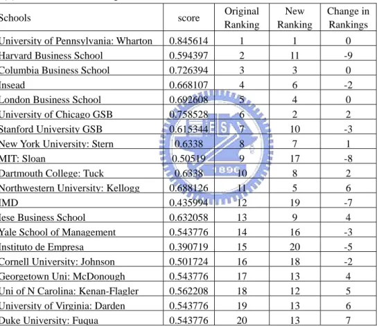
(33) After applying the hard data to the Common-Weight Model, Tables 3.3a and 3.3b displays the results. Table 3.3a shows the new score and the new rankings for these twenty universities along with the original rankings and Table 3.3b shows the new weightings. Please note that due the number of the original criteria, only five were selected from the original twenty criteria. Hence the result varied greatly.. Table 3.3 Results from Common-Weight Model. (a) New scores and rankings Schools University of Pennsylvania: Wharton Harvard Business School Columbia Business School Insead London Business School University of Chicago GSB Stanford University GSB New York University: Stern MIT: Sloan Dartmouth College: Tuck Northwestern University: Kellogg IMD Iese Business School Yale School of Management Instituto de Empresa Cornell University: Johnson Georgetown Uni: McDonough Uni of N Carolina: Kenan-Flagler University of Virginia: Darden Duke University: Fuqua. score. Original Ranking. New Ranking. Change in Rankings. 0.845614 0.594397 0.726394 0.668107 0.692608 0.758528 0.615344 0.6338 0.50519 0.6338 0.688126 0.435994 0.632058 0.543776 0.390719 0.501724 0.543776 0.562208 0.543776 0.543776. 1 2 3 4 5 6 7 8 9 10 11 12 13 14 15 16 17 18 19 20. 1 11 3 6 4 2 10 7 17 8 5 19 9 16 20 18 13 12 13 13. 0 -9 0 -2 0 2 -3 1 -8 2 6 -7 4 -3 -5 -2 4 5 6 7. (b) New weightings obtained from Common-Weight Model. Original Weightings Normalized original weightings New weightings Change (%). Weighted salary Salary (US$) increase (%) 0.2 0.2 0.303030303 0.303030303 0.291382783 0.243472234 -1.16% -5.96%. 22. International Faculty with mobility rank doctorates (%) 0.06 0.05 0.09090909 0.07575758 0.27496259 0.13661036 18.41% 6.09%. FT research rank 0.1 0.151515 0.053572 -9.80%.

(34) By studying both tables, it is clear that the criterion “International Mobility Rank” has increased its weighting by more than double of its original weightings and criteria other than “Weighted Salary” has changed about 6% to 10% each. These changes have effected the new extremely. In the new ranking, half of the universities have shifted their rankings for more than 4 spots. Harvard and MIT have shifted 9 spots and 8 spots accordingly. Harvard has dropped 9 spots in ranking due to the fact that it has the lowest value in “International Mobility Rank”, which is accounted for 27.50% of the total score. MIT has dropped 8 spots because it has the second lowest score on “International Mobility Rank” and fourth lowest score on “Salary Increase %”, which accounted for 24.35%.. After applying the statistical t-test, the P value was found to be 0.8919, which means the differences between the original rankings and the new rankings are considered to be not statistically significant. Hence the result from the Common-Weight Model is acceptable statistically.. 3.2. 3D Spherical Model. In last section, the weights for each criterion were generated by the model, as well as the rankings. The model will calculate the coordinates of each DMU based on the weightings and project them onto a 3D ball. To insure the correctness of the 23.

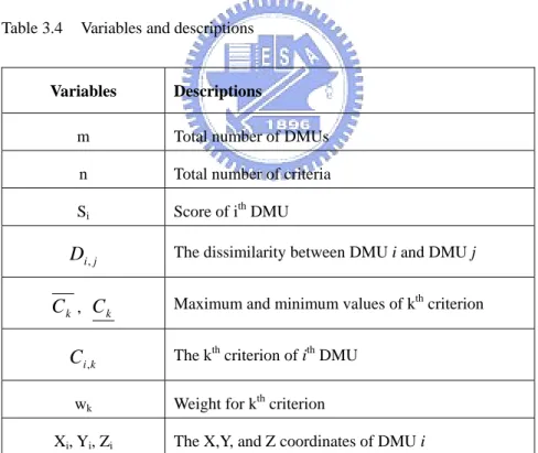
(35) mapping and the correlations between each DMU, the concept of dissimilarity is used in the calculation of the coordinates. Dissimilarity is the degree of difference between subjects. The general calculation method for dissimilarity will be discussed later in this section.. Table 3.4 lists the variables used in 3D Spherical Model and their meanings. Note that all the radius of the 3D balls is set to 1, and an ideal solution will be projected onto the North Pole. Ideal solution is an imaginary DMU that has the maximum value for each of its criterion. The purpose of this ideal DMU, as the standard, is to help the comparison process.. Table 3.4. Variables and descriptions. Variables. Descriptions. m. Total number of DMUs. n. Total number of criteria. Si. Score of ith DMU. Di , j. The dissimilarity between DMU i and DMU j. Ck , Ck. Maximum and minimum values of kth criterion. Ci ,k wk Xi, Yi, Zi. The kth criterion of ith DMU Weight for kth criterion The X,Y, and Z coordinates of DMU i. The Xi, Yi, and Zi are the actual coordinates of the DMUs on the 3D ball. Also, because the distances between DMUs on the 3D ball are not exactly the same as the 24.

(36) values of dissimilarities, we minimize the error between these two values to obtain the closest solution (Equation 3.8). With this solution, the projection of the points on the ball will be able to represent the relationships of the DMUs.. 3D Spherical Model (Model 2): m. MIN. m. ∑∑ ( X i =1 j >i. i. − X j ) 2 + (Yi − Y j ) 2 + ( Z i − Z j ) 2 − Di2, j. (3.8). Subject to: n ⎛ S i = ∑ ⎜ wk ⎜ k =1 ⎝. ⎛ Ci ,k − C k ∗⎜ ⎜ Ck − Ck ⎝. n ⎛ Di , j = 2 ∗ ∑ ⎜ wk ⎜ k =1 ⎝. ⎞⎞ ⎟⎟ ⎟⎟ ⎠⎠. ⎛ C i ,k − C j ,k ∗⎜ ⎜ C −C k ⎝ k. (3.9). ⎞⎞ ⎟⎟ ⎟⎟ ⎠⎠. (3.10). X i2 + Yi 2 + Z i2 = 1 , ∀ i. (3.11). Yi = 2S i − S i2 , ∀ i. (3.12). The objective of this model is to let the dissimilarity between two DMUs represents the distance between two DMUs. This is accomplished by minimizing the difference between the straight line distance of two DMUs and their dissimilarity value.. Equation 3.9 is the function to calculate score, which is the same as equation 3.7. Equation 3.10 calculates the dissimilarity between DMU i and DMU j. The largest possible value for Di , j is. 2 , because when one DMU is the ideal solution, which. have all the maximum value for each criterion, and the other DMU is the worst possible DMU, which must have minimum value for each criterion. Since the ideal 25.

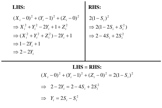
(37) solution will be at the North Pole and the worst possible solution will be on the equator. The straight line distance from the North Pole to the Equator on a ball with radius of 1 will be 2 . Similarly, if two DMUs are exactly the same, thought it is not likely to happen, the numerator will become 0, and so the Di , j will be 0.. Equation 3.11 is to ensure that every point is on the surface of the ball. And equation 3.12 defines the relationship between the Y coordinates and the score. To explain this equation, there is a proposition to discuss, as stated below.. Proposition 1: Yi. =. 2 ∗ S i − S i2 , ∀ i. (3.13). Proof:. ( X i − 0) 2 + (Yi − 1) 2 + ( Z i − 0) 2 = ( 2 ∗ Di ,* ) 2 = 2(1 − S i ) 2. (3.14). 2 − 2Yi = 2(1 − 2 S i + S i2 ). (3.15). Yi = 2S i − S i2. (3.16). In this proposition, Di ,* in equation 3.14 represent the dissimilarity between DMU i and the ideal solution. The original equation that calculates the distance between two points was changed to the current form, ( X i − 0) 2 + (Yi − 1) 2 + ( Z i − 0) 2 , since the ideal solution has the coordinate of (0, 1, 0). Equation 3.14 can be verified with (ideal solution, worst possible solution) pair and (ideal solution, best possible solution) pair. When these two pairs of DMUs are plugged in 3.165, they both hold. Hence, equation 3.14 is further simplified to 3.15 and finally 3.16. The simplification processes are shown as below.. 26.

(38) LHS:. RHS:. ( X i − 0) 2 + (Yi − 1) 2 + ( Z i − 0) 2. 2(1 − S i ) 2. ⇒ X i2 + Yi 2 − 2Yi + 1 + Z i2. ⇒ 2(1 − 2S i + S i2 ). ⇒ ( X i2 + Yi 2 + Z i2 ) − 2Yi + 1. ⇒ 2 − 4 S i + 2 S i2. ⇒ 1 − 2Yi + 1 ⇒ 2 − 2Yi. LHS = RHS: ( X i − 0) + (Yi − 1) 2 + ( Z i − 0) 2 = 2(1 − S i ) 2 2. ⇒ 2 − 2Yi = 2 − 4 S i + 2 S i2 ⇒ Yi = 2 S i − S i2. By applying the model to the example from section 3.1, we obtain the result shown in Table 3.5. Table 3.5. Coordinates for each universities. Schools Ideal Solution University of Pennsylvania: Wharton Harvard Business School Columbia Business School Insead London Business School University of Chicago GSB Stanford University GSB New York University: Stern MIT: Sloan Dartmouth College: Tuck Northwestern University: Kellogg IMD Iese Business School Yale School of Management Instituto de Empresa Cornell University: Johnson Georgetown Uni: McDonough Uni of N Carolina: Kenan-Flagler University of Virginia: Darden Duke University: Fuqua. score. New Ranking. x. y. z. 1 11 3 6 4 2 10 7 17 8 5 19 9 16 20 18 13 12 13 13. 0 -0.21658096 -0.41597168 -0.36376656 -0.32914496 -0.32199465 -0.33056332 -0.49832929 -0.45945342 -0.65293543 -0.49305753 -0.41447314 -0.73131613 -0.12768982 -0.58187571 -0.36325638 -0.65438051 -0.53405605 -0.49102552 -0.60957381 -0.52498427. 1 0.97616496 0.83548655 0.92514002 0.88984704 0.90551026 0.94169144 0.85203969 0.86589755 0.75516299 0.86589755 0.90273451 0.68189761 0.86461893 0.79185975 0.62877684 0.75172065 0.79185975 0.8083381 0.79185975 0.79185975. 0 0.013952 0.359068 0.108581 -0.31597 -0.27635 -0.06281 0.160301 -0.1978 0.058345 0.084355 -0.11525 0.0139 -0.48593 0.185415 -0.68752 -0.08187 -0.29621 -0.32478 0.037127 -0.31201. 1 0.845613979 0.594397421 0.726394479 0.66810701 0.692608172 0.758528351 0.615343904 0.633799985 0.505189925 0.633799985 0.688125846 0.435994334 0.63205834 0.543776095 0.390719143 0.501723624 0.543776095 0.562207931 0.543776095 0.543776095. 27.

(39) As previously mentioned, the ideal point is a point formed by setting the value of each of its criterion to the maximum value found from hard data. This point will lie on the North Pole with coordinates of (0, 1, 0) and score of 1. The worst point will be A4, with coordinates of (0.99127, 0, 0) and score of 0. With this example, it is coincident that the ideal solution is same as A1 and the worst point A4 is lying on the equator. Despite these facts, the distances between each point are shown in Table 3.6. These numbers also represent the dissimilarity between each DMU.. Table 3.6. Dissimilarity matrix. A0. A1. A2. A3. A4. A5. A6. A7. A8. A9. A10. A11. A12. A13. A14. A15. A16. A17. A18. A19. A20. A0. 0. 0.22. 0.57. 0.39. 0.47. 0.43. 0.34. 0.54. 0.52. 0.7. 0.52. 0.44. 0.8. 0.52. 0.65. 0.86. 0.7. 0.65. 0.62. 0.65. 0.65. A1. 0.22. 0. 0.49. 0.27. 0.45. 0.32. 0.12. 0.33. 0.32. 0.48. 0.3. 0.26. 0.58. 0.52. 0.51. 0.81. 0.49. 0.43. 0.4. 0.43. 0.43. A2. 0.57. 0.49. 0. 0.45. 0.67. 0.65. 0.52. 0.27. 0.56. 0.27. 0.35. 0.48. 0.59. 0.99. 0.42. 1.03. 0.41. 0.7. 0.68. 0.4. 0.6. A3. 0.39. 0.27. 0.45. 0. 0.55. 0.42. 0.18. 0.28. 0.2. 0.31. 0.15. 0.36. 0.47. 0.61. 0.26. 0.91. 0.32. 0.37. 0.47. 0.26. 0.49. A4. 0.47. 0.45. 0.67. 0.55. 0. 0.26. 0.38. 0.42. 0.5. 0.45. 0.55. 0.22. 0.44. 0.52. 0.67. 0.57. 0.48. 0.57. 0.43. 0.55. 0.35. A5. 0.43. 0.32. 0.65. 0.42. 0.26. 0. 0.25. 0.48. 0.26. 0.47. 0.41. 0.21. 0.59. 0.34. 0.47. 0.49. 0.33. 0.31. 0.2. 0.41. 0.23. A6. 0.34. 0.12. 0.52. 0.18. 0.38. 0.25. 0. 0.35. 0.22. 0.36. 0.23. 0.19. 0.49. 0.47. 0.39. 0.74. 0.36. 0.3. 0.3. 0.3. 0.31. A7. 0.54. 0.33. 0.27. 0.28. 0.42. 0.48. 0.35. 0. 0.38. 0.2. 0.23. 0.29. 0.34. 0.8. 0.5. 0.86. 0.31. 0.53. 0.51. 0.34. 0.43. A8. 0.52. 0.32. 0.56. 0.2. 0.5. 0.26. 0.22. 0.38. 0. 0.38. 0.26. 0.39. 0.53. 0.43. 0.25. 0.74. 0.25. 0.2. 0.29. 0.29. 0.31. A9. 0.7. 0.48. 0.27. 0.31. 0.45. 0.47. 0.36. 0.2. 0.38. 0. 0.19. 0.26. 0.37. 0.81. 0.34. 0.8. 0.19. 0.47. 0.46. 0.22. 0.37. A10. 0.52. 0.3. 0.35. 0.15. 0.55. 0.41. 0.23. 0.23. 0.26. 0.19. 0. 0.34. 0.41. 0.68. 0.31. 0.85. 0.19. 0.35. 0.41. 0.17. 0.43. A11. 0.44. 0.26. 0.48. 0.36. 0.22. 0.21. 0.19. 0.29. 0.39. 0.26. 0.34. 0. 0.4. 0.55. 0.56. 0.57. 0.35. 0.43. 0.29. 0.4. 0.21. A12. 0.8. 0.58. 0.59. 0.47. 0.44. 0.59. 0.49. 0.34. 0.53. 0.37. 0.41. 0.4. 0. 0.83. 0.66. 0.79. 0.43. 0.51. 0.57. 0.42. 0.48. A13. 0.52. 0.52. 0.99. 0.61. 0.52. 0.34. 0.47. 0.8. 0.43. 0.81. 0.68. 0.55. 0.83. 0. 0.62. 0.34. 0.66. 0.44. 0.44. 0.61. 0.53. A14. 0.65. 0.51. 0.42. 0.26. 0.67. 0.47. 0.39. 0.5. 0.25. 0.34. 0.31. 0.56. 0.66. 0.62. 0. 0.92. 0.27. 0.38. 0.53. 0.25. 0.55. A15. 0.86. 0.81. 1.03. 0.91. 0.57. 0.49. 0.74. 0.86. 0.74. 0.8. 0.85. 0.57. 0.79. 0.34. 0.92. 0. 0.68. 0.54. 0.44. 0.78. 0.43. A16. 0.7. 0.49. 0.41. 0.32. 0.48. 0.33. 0.36. 0.31. 0.25. 0.19. 0.19. 0.35. 0.43. 0.66. 0.27. 0.68. 0. 0.28. 0.28. 0.21. 0.28. A17. 0.65. 0.43. 0.7. 0.37. 0.57. 0.31. 0.3. 0.53. 0.2. 0.47. 0.35. 0.43. 0.51. 0.44. 0.38. 0.54. 0.28. 0. 0.19. 0.35. 0.22. A18. 0.62. 0.4. 0.68. 0.47. 0.43. 0.2. 0.3. 0.51. 0.29. 0.46. 0.41. 0.29. 0.57. 0.44. 0.53. 0.44. 0.28. 0.19. 0. 0.46. 0.09. A19. 0.65. 0.43. 0.4. 0.26. 0.55. 0.41. 0.3. 0.34. 0.29. 0.22. 0.17. 0.4. 0.42. 0.61. 0.25. 0.78. 0.21. 0.35. 0.46. 0. 0.48. A20. 0.65. 0.43. 0.6. 0.49. 0.35. 0.23. 0.31. 0.43. 0.31. 0.37. 0.43. 0.21. 0.48. 0.53. 0.55. 0.43. 0.28. 0.22. 0.09. 0.48. 0. 28.

(40) The dissimilarity values represent the degree dissimilarity between any two DMUs. If the value is 1, then the DMUS are totally different. If the value is 0, then the two DMUs are exactly the same, so the coordinates of these two DMUs will be the same as well. The school name has been replaced by variables due to the size of the dissimilarity matrix. A0 represents the Ideal Solution, A1 represents UPenn, A2 represents Harvard, and so on. Figure 3.2 is the projection of these points on a 3D ball by using the coordinates in Table 3.5.. Figure 3.2 3D ball with DMUs projected on the surface. Notice that the North Pole is the ideal point. The points with higher altitudes are points with higher rankings. Universities that are closer to the equator are the ones with lower ranking and scores. Figure 3.2 clearly shows that Instituto de Empresa has 29.

(41) the lowest ranking and IMD has the second lowest ranking, where University of Pennsylvania still has the best score.. 3.3. Clustering. In this step, the Clustering Model will assign each data point to a best fitting group. The DM can specify the number of groups he/she wants. The model will make sure that every group will have at least one data points.. Table 3.7 Variables. Variables and descriptions for Clustering Model Descriptions. m. Total number of DMUs. g. Total number of groups DM wants.. Tdisti. Total distance between data points to their center point in a group. grpij. Binary variable. grpij = 1 if DMU i belongs to group j.. ptij. Coordinate of DMU i. j = x, y, or z.. ctptij. Coordinate of Center Point i. j = x, y, z.. 30.

(42) Clustering Model (Model 3): g g ⎛ g Min⎜⎜ ∑ tdist i − ∑∑ ( x j − xk ) 2 + ( y j − y k ) 2 + ( z j − z k ) 2 j =1 k =1 ⎝ i =1. (. )⎞⎟⎟. (3.17). ⎠. Subject to: m. (. (. tdist i = ∑ grp ji * ( x pt j − xctpti ) 2 + ( y pt j − yctpti ) 2 + ( z pt j − z ctpti ) 2 j =i. grpij ∈ {0,1} g. ∑ grp j =1. j =1. (3.18) (3.19). ij. =1. ,. ∀i. (3.20). ij. ≥1. ,. ∀i. (3.21). m. ∑ grp. )). ( xctpti ) 2 + ( yctpti ) 2 + ( z ctpti ) 2 = 1. ,. ∀i. ( xi − x j ) 2 + ( y i − y j ) 2 + ( z i − z j ) 2 ≤ 2. (3.22) ,. ∀ i, j. (3.23). Equation 3.17 is the objective function, which tries to minimize the sum of distance between center points and data points in their group. Also, the distance between each center point has to be maximized to ensure that the clusters will be as far from each other as possible. Equation 3.18 calculates the distance between data points and center points in each cluster for every group. Equation 3.20 limits each DMU to belong to only one cluster. Equation 3.21 is to ensure every group has at least one DMU. Equation 3.22 is to force the center point to fall on the surface of the 3D ball. Finally, Equation 3.23 is to ensure that the longest distance between any two center points will be. 2.. From the 3D ball, we can group the DMUs by using the Clustering Model. The 31.

(43) By running the Clustering Model on this example, the grouping result is shown in Table 3.8. These twenty universities were grouped into three groups, where Harvard was grouped as the only member for group 1. Group 2 has 12 members and group 3 has 7. The number of members in a group was determined by the model automatically, but the user can specify the number of clustering groups.. Table 3.8 Groupings for universities Group 1. Group 2. Group 3. University of Pennsylvania: Wharton. 0. 0. 1. Harvard Business School. 1. 0. 0. Columbia Business School. 0. 0. 1. Insead. 0. 1. 0. London Business School. 0. 1. 0. University of Chicago GSB. 0. 1. 0. Stanford University GSB. 0. 0. 1. New York University: Stern. 0. 1. 0. MIT: Sloan. 0. 0. 1. Dartmouth College: Tuck. 0. 0. 1. Northwestern University: Kellogg. 0. 1. 0. IMD. 0. 1. 0. Iese Business School. 0. 1. 0. Yale School of Management. 0. 0. 1. Instituto de Empresa. 0. 1. 0. Cornell University: Johnson. 0. 1. 0. Georgetown Uni: McDonough. 0. 1. 0. Uni of N Carolina: Kenan-Flagler. 0. 1. 0. University of Virginia: Darden. 0. 0. 1. Duke University: Fuqua. 0. 1. 0. The grouping situation is shown as Figure 3.3. 32.

(44) Figure 3.3 Groupings for twenty universities. 33.

(45) 4. Iterative Ranking and Grouping In this chapter, the models presented in chapter 3 will be combined for the iterative ranking and grouping procedure. This new approach can be break into two parts and is give decision makers multiple chances to add preferences to the model. The first part of the iterative ranking and grouping model is the initial ranking process. This part is marked by the dotted line on the flow chart presented on the next page (Figure 4.1). This model will list the absolute dominance relationships in both table and preference graph format to the decision makers for them to add preferences. With the added preferences, the model will rank and group the DMUs and returns a set of weightings for criteria.. The second part of the iterative ranking and grouping model is shown by the shaded par of Figure 4.1. In this part, the DM will be presented with ranking result with grouping information. At this point, the DM can add preferences or change groupings for the DMUs. With the new input from the DM, the system will take the newly specified grouping information with preferences as input to recalculate the ranking and coordinates for the DMUs. The ranking is very likely to change due to DM’s grouping demand, so the coordinates and the weightings will surly be different from the previous iteration. The DM can choose to run this iterative ranking and grouping process as many times as she/he wants until she/he obtains the desired result.. 34.

(46) Figure 4.1. Flow chart for Iterative Ranking and Grouping Model. 35.

(47) Suppose John is a university student who is going to apply for MBA program. He knows the university in the United States very well and has four schools that he wants to apply to. However, his aunt is asking him to consider attending London Business School in England. John has no knowledge about this school, so he has decided to apply this Iterative Ranking and Grouping model to see how this London Business School will rank among his other four universities. Table 4.1 is the list of schools and part of data John obtained from Financial Times.. Table 4.1. Hard data on five universities John selected C1. School name. C2. C3. C4. C5. C6. Faculty Faculty Weighted Salary International with with International Country salary increase (%) students (%) doctorates doctorates faculty (%) (US$) (%) (%). A1 University of Pennsylvania: Wharton. USA. 1 0.965116279 0.197183099 0.741573034. 1. 0.176470588. A2 London Business School. UK. 0.635739. 0.76744186 0.887323944 0.876404494. 0.8. 0.694117647. A3 New York University: Stern. USA. 0.6243965. 1 0.042253521 0.449438202. 0.9. 0.294117647. A4 MIT: Sloan. USA. 0.832675 0.523255814 0.112676056 0.179775281. 0.6. 0.070588235. A5 University of Arizona: Eller. USA. 0.5. 0. 0 0.395348837 0.028169014. 0. The very first step after obtaining hard data is to create a tournament matrix. The purpose of tournament matrix is to identify the absolute dominant relationships in the matrix. Absolute dominance is said to exist when every criterion for DMU (Decision Making Unit) i is better than every criterion for DMU j. No matter what weightings we assign to these criteria in the future, the absolute dominance will still exist. Notice that the data will have to be processed prior to the ranking and grouping process so that all the data is set to be the larger the better. 36.

(48) In the tournament matrix T, the value of Tij is set to 1 if every criterion of Ti is smaller than Tj, which means Tj dominates Ti; otherwise a 0 will be recorded. Table 4.2 shows the variables used in Tournament Matrix Model, where it can automatically generate a tournament matrix to represent the absolute dominance relationships.. Table 4.2. Variables for Model 1. Variables. Descriptions. m. Total number of DMUs. n. Total number of criteria. ti,j. ti,j = 1 if DMU j is better than DMU i, else ti,j = 0. tci,j,k. Ck , Ck. tci,j,k is binary variable for pairwise comparison on criteria. tci,j,k = 1 if tci,k < tcj,k, else tci,j,k = 0. Maximum and minimum values of kth criterion. Ci,k. The kth criterion of ith DMU. wk. Weight for kth criterion. M. A large constant number. 37.

(49) Tournament Matrix Model: m. m. ∑∑. MIN. i =1 j =1. ti, j. (4.1). Such that. (Ci , k − Ck ). + tc j ,i , k. ≥. n − ∑ tci , j ,k + t j ,i. ≥. (Ck − Ck ) n. (C j , k − Ck ) (Ck − Ck ). 1. ,. ,. ∀ i, j , k. (4.2). ∀ i, j. (4.3). k =1. This model, will try to minimize the total number of t value, where t is a binary variable. The first constraint, equation 4.2, compares each criterion between every DMU. Since tci,j,k is set to be a binary variable and the value of. (Ci , k − Ck ) (Ck − C k ). is. normalized to between 0 and 1, tci,j,k will be set to one if Ci,k is smaller than Cj,k. The purpose of the second constraint is to fill in the values into the tournament matrix.. Following is the tournament matrix generated by this model.. Table 4.3. Tournament Matrix for Universities. A1. A2. A3. A4. A5. Sum. A1. 0. 0. 0. 0. 0. 0. A2. 0. 0. 0. 0. 0. 0. A3. 0. 0. 0. 0. 0. 0. A4. 1. 0. 0. 0. 0. 1. A5. 1. 1. 1. 1. 0. 4. 38.

(50) From Table 4.3 we can see that A4 (MIT) is dominated by A1 (U Penn) and A5 (Univ. of Arizona) is dominated by all other universities. These relationships will not change no matter what weightings are returned by the model.. Figure 4.2 Preference graph from Table 4.3. Aside from the tournament matrix, a preference diagram (Figure 4.3) can also be drawn to help John see the relationships between the schools. As shown on Figure 4.2, there are arcs that are not necessary. This is because Table 4.3 has redundant information. When the number of DMU and criteria grows, the redundant information may increase and make the preference graph very confusing and difficult to read. Hence, the extra information in tournament matrix will need to be removed by following Algorithm 1.. 39.

(51) Algorithm 1: For each base DMU in matrix T, sum the values in each row, so that the least dominant DMU will have the highest value. Take DMU with the lowest non-zero sum and call it R (the row number). If there are ties in the sum, pick the one with larger raw number. For row R, For each non-zero value on row R, do if there exist “1” on location TRC, then if TXR and TXC both are 1, then change TXC to 0 else do nothing Repeat with next DMU that has the next lowest sum or DMU that has the equal sum but next largest row number.. For example, the row with lowest non-zero sum will be row 4 in Table 4.3. Suppose we call this tournament matrix T, location T41 is set to be “1”, and row 5 has “1” at both T51 and T54. Hence, T51 needs to be set to “0”. This procedure has to be performed on the whole matrix to eliminate the extra information. The reduced matrix is shown in Table 4.4, and the new preference graph is shown in Figure 4.3.. Table 4.4 Reduced tournament matrix A1. A2. A3. A4. A5. A1. 0. 0. 0. 0. 0. A2. 0. 0. 0. 0. 0. A3. 0. 0. 0. 0. 0. A4. 1. 0. 0. 0. 0. A5. 0. 1. 1. 1. 0 Figure 4.3 New preference graph. 40.

(52) With the information reduced from tournament matrix, we can draw a preference graph (Figure 4.3). This graph can help the John to visualize the absolute relationships obtained from hard data and add preferences accordingly.. Figure 4.3 shows that A1>A4, A2>A5, A3>A5, and A4>A5. These dominance relationships are extracted from the hard data directly, so John can not change any of these relationships. There are still relationships that are either unclear or unable to determine from the hard data.. Now, John can add preference(s) by drawing two types of connecting lines on the preference graph for any two DMUs sets as the additional preference to help the model find optimal weightings for criteria. The first type is directed arrow, “Æ”. The head of the arrow can implied the “>” sign in math, which means the starting node is superior to the ending node. The second type of connecting lines is the dotted line, “- -“. If John connects two nodes with dotted line, this means that he thinks these two nodes should have the same ranking. At this point, John has decided not to add any preferences. He wants to wait until the results are returned from the model before he specifies any preferences.. Notice that he can only add one preference at a time. After one insertion, the corresponding value in the tournament matrix will be changed. Since the tournament matrix will record only the “greater” relationships, all the “equality” relationships will be incorporated with the objective function of the model during the weightings for criteria.. In order to keep the preference diagram free from cycles, after every preference 41.

(53) addition, the tournament matrix will need to undergo a “transitivity test”, which uses the technique presented by Gass. Since the matrix has size of m by m, all the diagonal values need be 0 for T3 up to Tm, by the theory Gass proposed. If any of the Tx has one or more non-zero diagonal value, the last added preference will be removed in order to keep the transitivity. If the new preference passed the transitivity test, the extra information will need to be removed by applying Algorithm 1 from last section to this new tournament matrix. The complete preference adding procedure can be seen from the flow chart (Figure 4.4).. Draw Preference Graph. Pass. Transitivity Test Fail. Remove last added preference. Add Preference. Yes. Add one Preference. Update Tournament Matrix. No. Common Weight Model. Figure 4.4 Flowchart for preference addition. After both the transitivity test and removal of extra information from the matrix, the Preference Diagram will be re-drawn and present to the John to add next preference. It is important that John adds preferences from the most important relationship to the least important ones, since with increasing number of preferences, the chance to get an intransitive relationship will increase as well.. This procedure will repeat until John has no more preferences to add. Given 42.

(54) John’s preferences, the model can use these preferences as part of the constraints to automatically produce weightings for each criterion. Table 4.5a shows the ranking results and Table 4.5b shows the weightings for each criterion.. Table 4.5 Results from initial run of the model (a). Ranking for five universities X. Y. Z. Score. Rank. A1. 0.1298738 0.990961946. 0.03357416. 0.904931317. 1. A2. 0.1687944 0.855201207. 0.490040133. 0.619475634. 3. A3. 0.3260319 0.841850725. 0.430105285. 0.602320135. 4. A4. -0.1002794 0.880834783. 0.462681456. 0.654796847. 2. A5. 0.1418996. 0.989881053. 0. 5. 0. (b) Weights for criteria. Weight. C1. C2. 0.74028. 0.15465. C3 0.001. C4 0.10206843. C5. C6. 0.001. 0.001. The weight for C1, which is the weighted salary, is weighted almost three-quarters of all attributes in the initial run of the model. The minimum value is not 0 because every criteria has to participate in the ranking process. However, due to the fact that every criterion has to be accounted in the score calculation, there are three criteria are with weights of 0.001.. Table 4.6. Grouping table for the initial result Group1. Group2. A1. 0. 1. A2. 0. 1. A3. 0. 1. A4. 1. 0. A5. 1. 0. Groupings can be seen from both Table 4.6 and Figure 4.5 shows the grouping 43.

(55) situation for these five schools. MIT and University of Arizona are being ranked in the same group, which John thinks is not quite logical. He can change the groupings for these schools at the first iteration of the ranking and grouping process.. Figure 4.5 Initial grouping situation represented on 3D ball. To specify the desired grouping, John believes that MIT should be in the same group as University of Pennsylvania, though he is not sure about the London Business School. He also thinks that New York University should be grouped in the same groups as University of Arizona. Hence, he modified the grouping table and obtained a new grouping table as shown in Table 4.7. 44.

(56) Table 4.7. New grouping table specified by John. Group1. Group2. A1. 0. 1. A2. 0. 1. A3. 1. 0. A4. 0. 1. A5. 1. 0. This table will then be one of the input values for the iterative ranking and grouping model to calculate the new rankings, weightings, and coordinates for the universities. Table 4.8a and Table 4.8b display the result from the first iteration. Although the ranking is still the same, other value have being changed. Criterion 6, Faculty with doctorates, is now weighted slightly than the previous run.. Table 4.8 Results form the groupings specified by John (a) New score and rankings for universities X. Y. Z. Score. Rank. A1. 0.1794657 0.983523545. 0.021760375. 0.871639354. 1. A2. 0.1817976 0.844442538. 0.503851591. 0.605592264. 3. A3. 0.3387656 0.835473124. 0.432692181. 0.594380873. 4. A4. 0.301143. 0.878376667. 0.371170188. 0.65125463. 2. A5. 0.5546003. 0. 0.832116892. 0. 5. (b) New weighting for criteria. Weight. C1. C2. C3. C4. C5. C6. 0.74518. 0.1581203. 0.001. 0.0336. 0.001. 0.0611. Now John can look at the 3D graph (Figure 4.6) that displays the groupings he specified.. 45.

(57) Figure 4.6 New coordinates and groupings for the universities. Because the points for New York University and University of Arizona are far apart, John is not quite satisfied with the current ranking and grouping result. He has noticed that New York University has lower score than MIT and he has heard some rumor form his friend which changed his perspective on MIT. So he now adds a preference which states that the score of New York University should be higher than the score of MIT.. 46.

(58) Although he can still change the groupings again, but he is satisfied with the groupings she set. Hence the grouping table will still be the input value for the model. Under the constraint section, we need to add a constraint that says “score of NYU is higher than the score of MIT”. After this preference is added, Table 4.9 shows the results for second iteration.. Table 4.9 Results with preference (a) New score and rankings for universities X. Y. Z. Score. Rank. A1. 0.1361369 0.786711637. 0.602122535 0.538168469. 1. A2. 0.127071 0.777934447. 0.615362452 0.528761681. 2. A3. 0.5582307 0.761262615. 0.329935869 0.511392401. 3. A4. 0.6453213 0.450878182. 0.616659831 0.258972458. 4. A5. 0.8251283. 0.564945379. 5. 0. 0. (b) New weighting for criteria. Weight. C1. C2. 0.21127. 0.4750437. C3 0.001. C4 0.001. C5 0.001. C6 0.310691. Notice that the score for A3 (NYU) is much higher than the score of A4 (MIT). By add this one constraint, not only the ranking has changed, but also the weightings has changed dramatically. Notice that the first criterion’s weighting was more than 0.7, and now has dropped to around 0.21. This means that C1 (weighted Salary) is a strong attribute for MIT. Now that NYU is better than MIT, the weighting for weighted salary is lowered. On the country, the weightings for salary increase (C2) and faculty with doctorates (C6) has increased in a great deal.. 47.

(59) Figure 4.7 New coordinates for the university with John’s preference.. With John’s preference, the score of MIT has dropped considerably lower than U Penn, London Business School, and NYU.. If John has no more preference to add, this will be the final ranking for him to use as a reference to help him decide whether he should apply for London business School. If John admires students who are attending University of Pennsylvania, then perhaps John should really consider applying to London Business School. However, If John he can still adds more preferences and run the model iteratively. 48.

(60) Remark This model provides many chances for the decision makers to add their opinions and runs it iteratively. By this approach, the final result will be logically consistent with what the decision makers have in mind, because this model ranks DMUs based on the preferences provided by decision makers. Hence, the result should be very useful for the DM in further decision making processes.. 49.