基於人類視覺系統特性之視訊編碼

國

立

交

通

大

學

資訊科學與工程研究所

碩

士

論

文

基 於 人 類 視 覺 系 統 特 性 之 視 訊 編 碼

Human Visual System Based Bit Allocation for Video Coding

研 究 生：張文潔

指導教授：蔡淳仁 教授

基於人類視覺系統特性之視訊編碼

Human Visual System Based Bit Allocation for Video Coding

研 究 生：張文潔 Student：Wen-Chieh Chang

指導教授：蔡淳仁 Advisor：Chun-Jen Tsai

國 立 交 通 大 學

資 訊 科 學 與 工 程 研 究 所

碩 士 論 文

A Thesis

Submitted to Institute of Computer Science and Engineering College of Computer Science

National Chiao Tung University in partial Fulfillment of the Requirements

for the Degree of Master in

Computer Science June 2006

Hsinchu, Taiwan, Republic of China

基於人類視覺特性之視訊編碼

摘要

本論文主旨在於利用人類視覺特性設計視訊編碼中的位元配置方式，以期達 到較佳的視覺品質。論文中提出的方法著重於人類視覺中的早期視覺處理，並由 於低階視域的運作行為較為一般性，所以依低階視域特性設計預測失真的公式。 在視訊編碼中，通常視訊複雜度分析是設計位元配置的核心考量。在本論文中， 視訊複雜度進一步分解為視覺複雜度與編碼複雜度。視覺複雜度直接影響流量控 制機制，在視覺重要性較高的地方分配較多的位元，在可以承受較大失真的地方 配置較少的位元。論文中並利用SSIM作為以感覺為基礎的客觀失真測量方式來評 量所提出的基於視覺系統設計之流量控制機制。在H.264 JM7.6上的實驗結果顯 示，論文中提出的方法與JM7.6中的參考流量控制機制比較之下，提案方法在所 有測試案例中皆有較好的表現，能夠達到較佳的視覺品質並降低所使用的位元 數。

Human Visual System-Based

Bit Allocation for Video Coding

Abstract

This paper proposes a video bit allocation scheme based on perceptual model of human visual systems for better visual quality. The proposed algorithm focuses on human early vision processes and formulates a distortion measure based on low-level vision behavior because of its generality. Generally speaking, video complexity analysis is the core component of the bit-allocation decision of a video encoder. In this thesis, video complexity is further decomposed into visual complexity and coding complexity. The visual complexity analysis directs the rate control model to assign more bits to the regions with visual importance, and assign fewer bits to the regions that could tolerate larger distortion. The proposed visual-based rate control algorithm is evaluated using a perceptual-based object distortion measurement called structural similarity index (SSIM) which approximates the perceived image distortion. Experiments based on H.264 JM7.6 shows that in comparison with the reference rate control in JM7.6, The proposed method has better performance with higher SSIM numbers and lower bitrate in all test cases.

Acknowledgement

I would like to express my gratitude to all those who gave me the possibility to complete this thesis. First, I would especially like to thank my advisor, Professor Chun-Jen Tsai. He gives me a lot of motivation and suggestions. Also, he encourages me to think in various viewpoints to analyze the issue and create new ideas. Then, I appreciate the great help and comments from my seniors, juniors, and classmates. During these days at National Chiao-Tung University, I enjoy the moments studying with all MMES Lab members. Finally, I would like to thank my family for their supports and encouragement.

Content

1.

Introduction...10

2.

Related Work...14

2.1. Rate Control Algorithms without Perceptual Models...14

2.2. Properties of Human Visual Systems...15

2.2.1. Contrast Sensitivity Function...16

2.2.2. Luminance masking ...17

2.3. Perceptual Based Bit Allocation for Video Coding ...18

2.4. Shortcomings of Current Work ...19

3.

Study and Analysis of Rate Control Theories....21

3.1. Hybrid Motion compensation/DCT Video Coding Model ...21

3.2. Rate Distortion Theory ...23

3.2.1. Rate Distortion Function...24

3.2.2. Rate Distortion Function for Gaussian Source ...26

3.3. Rate control in H.264...27

3.3.1. GOP Level Rate Control ...28

3.3.2. Picture Level Rate Control...29

3.3.3. Basic Unit Level Rate Control...33

3.4. Contrast Sensitivity Function Analysis...35

3.5. Perceptual-Based Objective Video Quality Assessment...38

4.

Proposed Rate Control Framework ...45

4.1. Investigation of Video Complexity Measures ...45

4.2. Analysis of Visual Complexity...48

4.2.1. Basics of Spatial Derivatives ...49

4.2.2. Spatial Contrast Sensitivity...51

4.3. Proposed Rate Control Scheme ...57

5.

Experimental Results...62

5.1. Results of Visual Complexity ...62

5.2. Results of Proposed Bit Allocation Scheme ...65

List of Figures

Figure 1. Encoding process ...22

Figure 2. Rate control flow chart...34

Figure 3. The Mannos-Sakarison CSF and the Ahumada CSF ...37

Figure 4. Comparisons of four different CSFs ...38

Figure 5. Comparison between SSIM and PSNR on high quality images ...42

Figure 6. Comparison between SSIM and PSNR on distorted images ...43

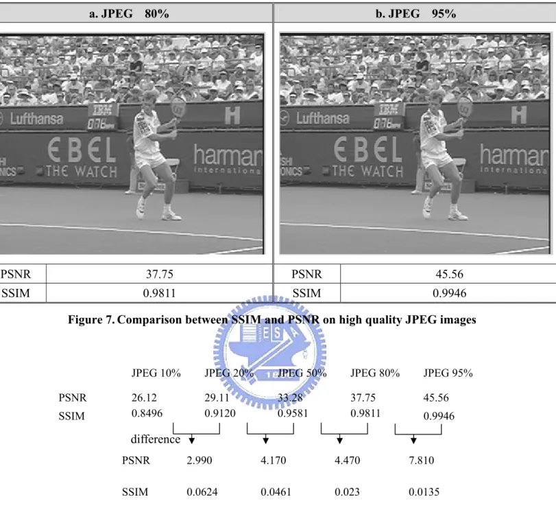
Figure 7. Comparison between SSIM and PSNR on high quality JPEG images....44

Figure 8. Laplacian masks...50

Figure 9. Filters in different domain ...51

Figure 10. CSF filtering of images...53

Figure 11. Comparisons of the proposed CSF with other CSFs ...56

Figure 12. result of visual complexity computation...57

Figure 13. Graphs of ln(1/αD) and its second-degree Taylor approximation ...59

Figure 14. Block diagram of the proposed rate control model...60

Figure 15. (a)Original 10th frame in Funfair and (b)Distortion tolerance map ....63

Figure 16. (a)Original 3rd frame in Foreman and (b)Distortion tolerance map....63

Figure 17. (a)Original 24th frame in Foreman and (b)Distortion tolerance map..64

Figure 18. SSIM performance comparison of STEFAN ...67

Figure 19. SSIM performance comparison of FUNFAIR ...68

List of Tables

1. Introduction

Video compression is an important topic in multimedia applications nowadays. Since the data volume of digitalized video is large for most storage and transmission systems, compression is essential for video applications. For the past decade, the technology of video compression has created many new multimedia applications, such as DVD movies, digital television, and video conferencing. Popular video coding standards adopt a lossy approach where some data from the video source are discarded during compression due to limited bandwidth or storage constraints. The process that determines which part of the source data should be discarded is called rate control.

A rate control algorithm allocates target bits for each coding unit and adjusts coding parameters to achieve the target bitrate. Rate control schemes can be categorized into two groups, which are variable-bit-rate (VBR) control and constant-bit-rate (CBR) control. The VBR rate control scheme attempts to maintain constant video quality by allocating different amount of bits to different segment of video data based on their entropy. As a result, the compressed bitstream data rate varies across time. On the other hand, the CBR rate control tries to minimize the variations of compressed bitstream data rate in order to fulfill the bandwidth constraints from video delivery channel, or the playback device capability constraints (i.e. the processing speed in bits-per-second). A side effect of this rate control approach is that the resulting video quality may vary across time. In practice, the rate control algorithm selects a proper quantization parameter in order to produce a bitstream that fulfills the application constraints.

In existing encoding models, most of them analyze video data complexity for bit allocation and rate control. The complexity (or loosely speaking, entropy) is computed either by the mean absolute difference (MAD) measure of the residual data for inter-predicted frame or by the standard deviation for intra-predicted frames. Although MAD can reasonably represent the coding complexity of a region of video data, it does not sufficiently capture the perceptual importance of the data. Since in most video compression applications, human eyes are the final judgment of quality, perceptual models of human vision systems must be considered for better bit allocation.

Although human perceptual models have been successfully used for audio coding [28], it has not been popular for either still image coding or video coding. You probably do not need a complicated model for still image coding since the data amount is small. However, for motion picture coding, perceptual models are not used mainly because the behavior of human vision systems is very difficult to put into equations. Some coding schemes are proposed for content-based video compression since conceptually, human high-level visions work on objects instead of pixels [29][31] . A general method alone this line of thinking is to decompose a video sequence into foreground and background representations, and reduce the coding bitrate of the background data. However, we do not agree with this approach since the regions which attract human attention are most likely related personal experiences and are different from person to person. Therefore, our proposed algorithm focuses on human early vision processes [7] and tries to formulate a distortion measure based on low-level vision behavior because of its generality.

In this thesis, a rate control algorithm based on human visual system properties is proposed. The proposed rate control model of visual complexity is composed of

visual texture complexity and temporal complexity. A modified contrast sensitivity function is proposed to estimate the visual texture complexity. The visual texture complexity map represents visual distortion sensitivity of each macroblock and is incorporated into the proposed rate control model.

One critical issue in developing a perceptual model-based rate control algorithm is about how to judge the quality of a coded bitstream. The most common objective quality measurement for lossy compressed video is the peak signal-to-noise ratio (PSNR) measure. Nevertheless, researches show that the value of PSNR does not completely agree with the perceptual quality evaluated by human eyes [30]. That is the reason why International Standardization Organizations (ISO) Motion Picture Expert Group (MPEG) only uses subjective viewing tests for the evaluation of the performance of proposals for various new technology call-for-proposals (CfPs) and for final verification tests of a new prospective standard. Unfortunately, subjective viewing tests are difficult to conduct and are subject to bias if the tests are no done properly. In this thesis, we investigate an objective distortion measurement called structural similarity index (SSIM) which approximates the perceived image distortion. From our experiments, SSIM is clearly more consistent with perceptual quality than PSNR is. The proposed visual-based rate control algorithm is evaluated using the SSIM measure.

The organization of the thesis is as follows. Chapter 2 introduces some previous work of rate control schemes, including non-visual model-based and visual model based ones. Some theories and models of human visual systems are also presented in this chapter. Chapter 3 introduces mathematical for the theoretical foundations of the proposed solutions. The detail of the proposed algorithm is derived and presented in Chapter 4. The experimental results are shown in Chapter 5. Finally, some discussions

2. Related Work

As mentioned in chapter one, rate control algorithm of a video encoder throws away less important data that cannot fit into rate constraint of the target applications. All rate control algorithms are based on some Rate-Distortion (R-D) Models. An R-D model describes the tradeoff between quality (or distortion) and bitrate of a video codec. Ideally, a distortion measure that conforms to human visual behavior should be used to determine which part of the video source is more important than the others. However, human visual behavior is very difficult to model mathematically. Therefore, most published video rate control algorithms use some artificial distortion measures such as mean-square-error (MSE) or mean-absolute-error (MAE) instead.

The organization of this chapter is as follows. In section 2.1, we will first list some conventional video rate control algorithms which do not take into account human perceptual model. Section 2.2 investigates some published studies on human visual behaviors. In particular, we will focus on the contrast sensitivity function and the luminance masking effect since these features will be used in our proposed method. In section 2.3 we will take a look at several approaches, including, macroblock classification using edge detection information [4], the foveated approach by Lee et al.[20] and the visual distortion sensitivity index (VDSI) approach by C.W. Tang et al. [6].

2.1. Rate Control Algorithms without Perceptual Models

Different video codecs and video sequences have different Rate-Distortion (R-D) characteristics called R-D functions. At the core of any rate control algorithm is a parameterized R-D model that can be used to approximate the R-D function of the

target sequence by solving model parameters. Rate control algorithm describes the tradeoff between video quality and bit rate constraint. Different bit allocation algorithms are designed based on different R-D models. The distortion resulting from a lossy encoding process is related to the quantization parameter (QP) used during the quantization stage. In fact, the main purpose of establishing the R-D model and solving for the R-D function is to find the proper QP for each coding unit so that the smallest distortion given a rate constraint can be achieved. For example, the R-D model in MPEG-2 TM5 [16] is a simple linear function of rate and QP while in MPEG-4 Annex L [18], a more accurate second-order R-D model is proposed [17] .

In both the TM5 and the MPEG-4 Annex L methods, QP is considered a linear function of distortion. Although this simplifies the problem, it is nevertheless not accurate. In [19], Z. He and S. Mitra propose a linear model based on the percentage of zero coefficients in the quantized video data. They proposed the rate distortion function in ρ domain instead of the traditional quantization-step-size domain. It is shown that it is a linear relationship between coding bitrate and the percentage of zeros among the quantized DCT transform coefficients, denoted by ρ. The relation between quantization step size and ρ is a one-to-one mapping, and the mapping can be computed from the distribution of the transform coefficient. Therefore, as long as ρ is determined by the rate-ρ function, quantization parameter is designed by table look-up and bi-linear interpolation. Experiments show that this method is more accurate in matching the target bitrate. However, it does not take into account visual quality.

2.2. Properties of Human Visual Systems

of video quality, a video codec should take into account perceptual characteristics of the video data like audio codecs do [28]. Notice that Human Visual System (HVS) has many resolution limits, so one of the main objectives in design compression scheme is to represent the information that HVS can detect. Many experiments have been conducted to help understanding of HVS [1][7][34] , but it is very hard to develop a complete computational model for HVS due to its complexity. However, through the experiments, researchers analyzed many properties of HVS, such as the visibility threshold, and try to derive a generalized computational model for it. The visibility threshold, which is defined as the magnitude of the stimulus when it becomes just visible or just invisible, is an important feature for video coding.

2.2.1. Contrast Sensitivity Function

Contrast Sensitivity function (CSF) is an important issue of HVS-modeling. One of the many limits of eyes is that the visual system can not recognize the stimuli pattern when the frequency of stimuli is too high. This is due to the limited number of photoreceptors in human eyes [8]. The sensitivity of the eyes depends on the spatial frequency of luminance variations. This phenomenon can be characterized by the CSF. Many researchers proposed various forms of CSF [1][2][23]. Because CSF is a bandpass filter, many of the proposed function are composed of a high-frequency lobe minus a low-frequency lobe [9].

Mannos and Sakrison [1] proposed a computational CSF model and took the lead to introduce it as a distortion measure for image. Many later perceptual based coding researches adopt and modify this model [3][10] . The Mannos-Sakrison CSF model can be constructed through the following steps. First, it normalizes all luminance value by L/Lm, where Lm is the mean luminance, and considers the nonlinearity in

model the property that eyes are more sensitive to small variation in dark background than in light ones. Second, frequency domain image f(u,v) is computed by Fourier transform of the result image in first step. Third, (u,v) is the direction in the frequency domain and expressed in terms of cycles/degree based on the viewing distance of 36 inch, which is applied empirically for establishing Mannos-Sakrison CSF model as follows: 2 2 ) , ( :r u v u v frequency Spatial = + MS_CSF(r)= 2.6*[0.0192+0.144r]exp[-(0.144r)1.1] (1)

The Mannos-Sakrison CSF described above is a single channel model. Some researchers propose more complex model with multiple spatial frequency channel [2]. The multiple channel model compute channel output based on spatial frequency, spatial position, and orientation. These models are computationally very complex.

2.2.2. Luminance masking

The visual threshold of HVS has a strong dependence on the neighboring background luminance. The sensitivity which depends on the local mean luminance is called “light adaptation” or “luminance masking”. It is related to the well-known HVS property, Weber’s law. According to Weber’s law, the ratio of just visible luminance difference (∆L) to surrounding luminance (LB) is approximately constant from

medium to high luminance value [10][11] . This property describes that the visual perception is more sensitive to the contrast luminance then the absolute luminance. However, the Weber fraction (∆L/ LB) starts to increase nonlinearly with decreasing

less visible then that in medium luminance region.

Many studies have proposed perceptual model based on luminance masking. In [13], Safranek and Johnston performed some experiments and found the curve of sensitivity for varying background grey levels. CH Chou and YC Li [14] proposed a formula to fit the experimental results in [13]. The relationship corresponds to high luminance is modeled by linear function. This linear model matches the experimental results that the Weber fraction is constant from medium to high luminance value. Low background luminance (below 128) is modeled by root equation, which matches the experimental results that the Weber fraction starts to increase nonlinearly in low luminance.

2.3. Perceptual Based Bit Allocation for Video Coding

The bit allocation algorithm is used to arrange the distribution of target bits to minimize the distortion. In general bit allocation algorithms, quantization level of coding unit is computed based on the coding complexity [17], which is often approximated by mean absolute different (MAD). Several perceptual bit allocation models for video coding have been proposed in the literature. In [4], Tao presents a macroblock-level bit allocation algorithm based on the theoretical rate-distortion function for a Gaussian random variable with squared error distortion. A region classification scheme is included in the algorithm, which classify each macroblock into a perceptual class. Each class characterized by human visual perception has different visual importance. The classification classifies a macroblock into one of six perceptual classes, in descending order of noise sensitivity: (1) edge; (2) uniform with moderate; (3) uniform with either high or low intensity; (4) moderately busy; (5) busy; and (6) very busy. They classify a macroblock (MB) by performing Sobel edge

detection and computing the average of the variances of the four blocks in the MB. The human retina possesses a non-uniform spatial distribution of photoreceptors, hence the detectable local visual frequency bandwidth falls away from fovea. For this reason, Lee et al. [20] proposed the rate control algorithm for foveated video compression. Foveated image is created based on fixation point, which intersects the visual axis. The position of fixation point is determined in real-time by eye tracker. Foveated image is estimated the image formed on the human eye, and it is created by removing the undetectable high visual frequency based on the distance to the foveated point. In creating foveated image, the original image is transformed to curvilinear domain, where the size of the partial image is in inverse ratio with the distance to foveated point. The bit allocation algorithm is preformed in curvilinear coordinate. The number of target bits can be equally allocated into each unit region in the transformed image. Thus, the target bits are nonuniformly allocated in the foveated image in Cartesian coordinate.

In [5][6], Visual Distortion Sensitivity (VDS) is evaluated for bit-allocation. The proposed psychovisual model combines the motion attention model and the texture-structure model based on two types of edge detectors. The presented technique allocates fewer bits to regions allowing higher perceptual distortion.

2.4. Shortcomings of Current Work

The video coding techniques making use of human attention is designed based on the assumption that people often pay more attention to some specific visual object when viewing a video sequence. However, the areas which will attract one’s attention depend on personal experiences and differ from person to person. Therefore, it is not reasonable to artificially divide the video data into “foreground” and “background.”

As for foveated video compression, it is only suitable for real-time encoding and has to rely on extra instrument to track the position of visual fixation. Furthermore, most existing HVS-based video coding methods only apply very general concept of HVS properties without vast psychovisual experiments to back up the design.

Although, outside video coding domain, there are a lot of visual models derived from experiments in well-controlled conditions. These visual models are not specifically tuned for video coding applications. They have to be slightly modified in order to work for video coding.

3. Study and Analysis of Rate Control Theories

The goal of this thesis is to design a video rate control model based on visual behavior. Rate control algorithm allocates target bits for each coding unit and adjusts coding parameters to achieve the target bitrate and minimize the overall distortion of the entire sequence. First of all, before we design a perceptual model-based rate control algorithm, we must study the theory behind rate control algorithms. Existing rate control models are mostly derived from various R-D functions in information theory [36]. Secondly, to design a visual based coding system, it is important to understand the human visual system properties. Finally, since the goal of a rate control algorithm is to achieve better visual quality, it is essential to find a measure for quality assessment that is consistent with human perception.

In section 3.1, the prevalent block-based hybrid motion compensation/transform video encoding model is first introduced. In section 3.2, the concept of rate distortion theory and the application of the theory in source coding are described. Section 3.3 presents the reference implementation of rate control for H.264/AVC. In section 3.4, Contrast Sensitivity Function, which is a crucial HVS property, is analyzed. Finally, a perceptual model-based objective video quality measure is investigated in section 3.5.

3.1. Hybrid Motion compensation/DCT Video Coding Model

An important feature of a video sequence is that neighboring regions across successive frames tend to be highly correlated. Similarly, neighboring pixels within a video frame are highly correlated too. Each frame of a video sequence can be encoded

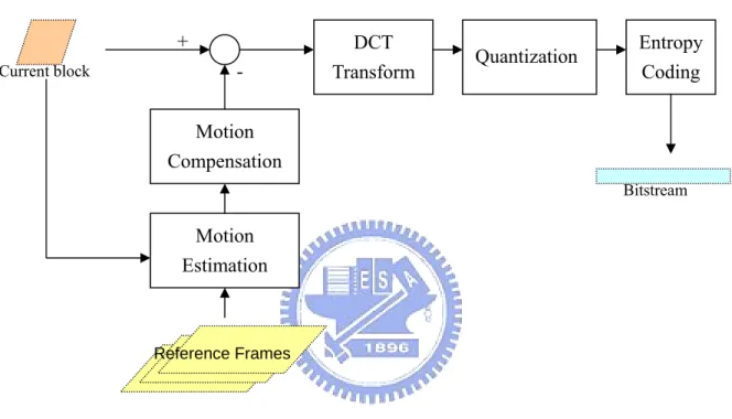
individually by using an image encoder (similar to a JPEG encoder), and it is called intra frame coding. However, video compression can achieve better performance if spatio-temporal redundancy in a video sequence is first eliminated. A general framework for hybrid motion compensation/DCT video coding scheme is shown in Figure 1

+ DCT Entropy

Figure 1. Encoding process

The first step is motion-compensated prediction. A current encoding block is compared with surrounding region of the previous reconstructed frame. The goal of this process is to find the best match region that most similar to the current block. Then the residual data is computed by subtracting the matching block, witch is also called reference block, from the current block. Accordingly, this process achieves exploiting the temporal redundancy.

The transform coding transforms the (residual) image from spatial domain into another domain in order to be more adaptable to compression. After performing DCT transform, the energy of image is concentrated into few critical coefficients, and other

Motion Estimation Current block Motion Compensation Quantization - Transform Coding Bitstream Reference Frames

coefficients with small value may be discarded without losing much accuracy. The transform stage does not achieve compression, but it separates the input data into different level in importance. Quantization is the step reducing the precision of coefficients in order to remove the less important transformed data and retain the important information. The DCT coefficient divides by quantization step size in implementation. The quantization step size is nearly the main parameter to control the compression ratio and quality in video codec. Entropy coding is a lossless compression scheme based on statistical properties of information to be encoded. The concept of entropy coding is to encode the most frequently occurring patterns with the least number of bits.

In video coding standard, there are three main types of encoding frame: I-frames, P-frame, and B-frame. I-frame is intra-coded without any motion compensated prediction. P-frame is inter-coded using previous frames as a reference for motion compensated prediction. B-frame is inter-coded using motion compensated prediction from two reference frames which temporally located before and after the current frame. Only I-frame and P-frame can be used as reference frames. I-frame is useful in re-synchronization, since it can be decoded independently without any reference. P-frame and B-frame provide better compression efficiency due to motion compensated prediction.

3.2. Rate Distortion Theory

The key mathematical formulation of lossy data compression is the rate distortion theory, which finds its root in information theory. Simply put, “rate” is the number of bits used to represent the input data, and “distortion” is the differences

between the input data and coded output signal. The problem is often formulated using a general communication system model, in which the source encoded by the source encoder and the channel encoder is transmitted through the channel to the receiver. The transmitted data is then decoded by the channel decoder and the source decoder, and reconstructed at the receiver. For a specific source, the Rate-Distortion (R-D) theory addresses the theoretical minimum bitrate R for a given distortion D.

3.2.1. Rate Distortion Function

The concept of rate distortion theory was first published by Shannon in 1948 [36], but until 1959 Shannon fully developed the fundamental theory for the rate distortion function of a source with fidelity criterion. In Shannon’s theory, the source symbols are given by the random sequence U with distribution {P(u), u∈U}, and the reconstructed symbols are given by the random sequence V with distribution {P(v), v∈V}. Shannon average mutual information expressed via entropy：

) | ( ) ( ) ; (V U E V EV U I = − dx x p x p x E( )= ∞ ( )log ( ) (2) 2

∫

−∞

where E(x) is the entropy of signal x. The conditional entropy E(U|V) represents the amount of missing information in the reconstructed signal. The mutual information between event V and U denoted by I(V;U) is the information provided about the event V by the occurrence of event U. For example, if the process of communication does not bring in any distortion and the reconstructed data is identical to the original data, then E(V|U) = 0, which means that V is ascertained giving input data U, and I(V;U) = E(V) = E(U).

The rate distortion function R(D) specifies the lower bound of the transmission bitrate for a given distortion D. The minimization is conducted for all possible mapping Q that satisfies the distortion constraint.

{

( )

}

min ) ( ) ( : I Q D R D Q Distortion Q ≤ = . ₍₃₎

The mutual information is considered as the rate in the rate distortion function. As the equation suggests, the mapping Q include the input sequence U and the reconstructed sequence V, and the computation of this function requires PDF P(U) of the input signal and the conditional PDF P(U|V) that minimizes rate for the given distortion D. Because the exact solution of this minimization problem is difficult to compute, there are many upper and lower bounds of this function based on different constraints [37], including the well-known “Shannon Lower Bound”, which is derived for a source U and the difference distortion measure d(u, v).

)) , ( ( ) ( ) ( ) (D R D E U E d U V R ≥ _LB = − (4)

By using the basic form with different distortion measures, it is easy to obtain two spatial cases. The first case uses the square error function as the distortion criterion, as follows. D(u, v) = (u – v)2 ) 2 ( log 2 ) ( ) ( ) (D R D E U ₂ eD R ≥ _LB = −1 π (5)

The second case uses the absolute error (i.e. the magnitude of errors) as the distortion criterion as follows.

D(u, v) = |u – v| ) 2 ( log ) ( ) ( ) (D R D E U ₂ eD R ≥ _LB = − (6)

3.2.2. Rate Distortion Function for Gaussian Source

As mentioned in section 2.1, R-D functions depend on both the codec and the video source, therefore, we must define a source model before we a discuss the R-D model for a video codec. The most well-known and commonly used source model is the memoryless Gaussian source. Memoryless source means that the signal is uncorrelated and independent. Assuming the source model is Gaussian distribution with variance σ2 and arbitrary mean µ, and the square error distortion measure is used the probability density function is

2 2_/2 ) ( 2 2 1 ) ( µ σ πσ − − = _e x x P . ₍₇₎

The entropy of the source signal with Gaussian distribution is

2 22 log 2 1 ) (p πeσ E = . (8)

From (7) and (8) [32], we have

D eD e eD e D R_LB 2 2 2 2 2 2 2 log 2 1 2 2 log 2 1 ) 2 ( log 2 1 2 log 2 1 ) ( σ π σ π π σ π = = − = . (9)

In order to make sure that the rate R is nonnegative, the equation can be written as ⎪⎩ ⎪ ⎨ ⎧ ≥ ≤ ≤ = = 2 2 2 2 2 2 , 0 0 , log 2 1 ) 0 , log 2 1 max( ) ( σ σ σ σ D D D D D R_LB . (10)

In this section, we introduced the general R-D function based on the square error distortion measure. The R-D model can be extended by the framework with different distortion measures or by content probability density function.

3.3. Rate control in H.264

Rate control algorithm allocates target bits for each coding unit and adjusts coding parameters to achieve the target bitrate. Block-based video coding schemes such as MPEG and H.26x controls the fineness of the encoded data and degree of entropy reduction by quantization step. The quantization parameter (QP) regulates how detailed the data is to be encoded. For a specific coding unit, when QP is small, the detail of this region is retained and the amount of used bits is large. As QP becomes large, the encoded data loss its precision and the amount of used bits is decreased. The rate control schemes depend on QP adjustment to satisfy the available bandwidth provided by the channel. A different way of describing the rate control process is called the bit allocation process since the finer the quantization step size is, the more bits will be allocated to the coding unit. In H.264, the bit allocation process consists of three different levels. That is, the group of picture (GOP) level, the picture level, and the optional basis unit level.

3.3.1. GOP Level Rate Control

In GOP level, rate control computes the total number of remaining bits for the rest of the picture in this GOP and determines the initial QP of the first stored picture (I-frame or P-frame).

Eq. (11) calculates the bits for the pictures after the jth picture (including No. j) in the ith GOP. The computation depends on instant available bit rate R, predefined frame rate f, the occupancy BV of the virtual buffer and the actual bits b used in the previously encoded picture.

1 1 ) 1 ( ) 1 , ( ) , ( ) 1 , ( ) 1 , ( ) , ( ) , ( ) , ( > = ⎪ ⎪ ⎩ ⎪⎪ ⎨ ⎧ + − × − − + − − − − × = j j j N f j i R j i R j i b j i T j i BV N f j i R j i T i i . (11)

The occupancy of the virtual buffer is update after encoding one picture as shown in Eq. (12). 1 ) 1 , ( ) 1 , ( ) 1 , ( ) , ( 1 ) , 1 ( 0 ) 1 , ( 1 > − − − + − = ⎩ ⎨ ⎧ = − = − j f j i R j i b j i BV j i BV other i N i BV i BV i . (12)

For the first picture (j = 1) in a GOP, it first computes the approximate available bits by multiplication of the number of pictures Ni in the ith GOP and the average

number of bits per frame, and then minus the occupancy BV of the virtual buffer to prevent buffer overflow. For the other pictures, it uses previously computed result of total target bits minus the actual bits used for the previously coded picture, and if the available bitrate varies, the function adjusts the average number of bits per frame.

The initial QP of the first GOP is predefined by the users. The I-frame and the first P-frame of first GOP are coded by a predefined quantization parameter QPinitial.

QPinitial should be selected based on the available channel bandwidth and frame rate.

The computation of initial QP of other GOPs must follow the constraint that the difference of first two quantization parameters of two consecutive GOPs is limited as in Eq. (13), ⎭ ⎬ ⎫ ⎩ ⎨ ⎧ ⎭ ⎬ ⎫ ⎩ ⎨ ⎧ ⎭ ⎬ ⎫ ⎩ ⎨ ⎧ − + − − − = − − − 15 , 2 min , 2 ) 1 , 1 ( min , 2 ) 1 , 1 ( max ) 1 , ( 1 1 1 i i i N NStored SumQP i QP i QP i QP , (13)

where SumQPi-1 is the sum of average quantization parameters of the stored pictures

in the previous GOP, and NStoredi-1 is the total number of stored picture in the

previous GOP. It computes the overall average quantization parameter of previous GOP in order to adjust current QP.

3.3.2. Picture Level Rate Control

In picture level (or called frame level) rate control, its contain three steps, which are determining target bits for each frame, computing the corresponding quantization parameter before encoding, and update parameters of rate distortion model after encoding one picture.

The first step is to determine the target bits for each picture. It has to dominate the buffer usage by target buffer level and the occupancy of the virtual buffer. If the scheme only supports the stored picture, the value of target buffer level is set by Eq. (14):

1 1 ) 2 , ( ) , ( ) 1 , ( ) 2 , ( ) 2 , ( > ⎪⎩ ⎪ ⎨ ⎧ − − = + = j N i BT j i BT j i BT i BV i BT i ⎟⎟ ⎠ ⎞ ⎜⎜ ⎝ ⎛ − − − × = − × − − = + ⇒ 1 1 1 ) 2 , ( ) 1 ( 1 ) 2 , ( ) 1 , ( i i N j i BV j N i BV j i BT BV(i,2) (14) .

The quantization parameter of the first frame in the GOP is determined by the GOP level rate control process, and the initial target buffer level BT(i,2) is set to the actual buffer occupancy after encoding first frame in the ith GOP. This value of target buffer level BT will be compared with the occupancy BV of the virtual buffer in the target bits computation. )) , ( ) , ( ( ) , ( ) , ( BT i j BV i j f j i R j i T = +γ × − . (15)

If the actual buffer occupancy is higher than the target buffer level, it may cause buffer overflow, then this function will reduce the target bits to match channel bandwidth. On the contrast, if the actual buffer occupancy is lower than the target buffer level, it may cause buffer underflow, and the solution is to increase the target bits. γ in (15) is constant and its typical value is 0.5.

The second Step is to compute the quantization parameter and perform the rate distortion model. The quantization step corresponding to the target bits is by computing the scalable quadratic distortion model proposed in [17]. The quadratic function is derived from the theoretical rate distortion model for Laplacian distributed source with the magnitude error distortion measure.

∞ < < ∞ − = _e− _{where x} x P x_, 2 ) ( α α . (16)

The magnitude error distortion measure is defined as d(u,v) = |u-v|. Eq. (16) can be used to derive a closed form solution of the R-D model:

α α α 1 0 , 1 , 0 , 1 ln ) ( max min = = < < ⎟ ⎠ ⎞ ⎜ ⎝ ⎛ = D D D where D D R . (17)

When Eq. (17) is expanded into a Taylor series, we have:

) ( 2 1 2 2 3 ) ( 1 1 2 1 1 1 ) ( 3 2 2 1 3 2 D R D D D R D D D R + − + − = + ⎟ ⎠ ⎞ ⎜ ⎝ ⎛ ₋ − ⎟ ⎠ ⎞ ⎜ ⎝ ⎛ ₋ = − − α α α α _. (18) (19)

Based oh the above derivation, a quadratic rate distortion model is formulated as Eq. (19): ) , ( ) , ( ) , ( 2 2 1 1 Q i j a Q i j a j i T _{= ×} − _{+ ×} − _.

In order to allow the R-D model scale with the video contents, the video coding complexity such as mean absolute error (MAD) is introduced. The R-D model is used to estimate the relation between quantization step and target bits for texture information, so the target bits for R-D model computation should not include the bit count used for coding the overhead of a frame.

) , ( ) , ( ) , ( ) , ( ) , ( 2 2 1 1 Q i j a Q i j a j i MAD j i H j i T − _{= ×} − _{+ ×} − _, (20)

where T(i,j) H(i,j) MAD(i,j) Q(i,j) a1, a2

total number of bits used for coding current picture j in ith GOP; number of bits used for coding the overhead of current frame;

mean absolute error, computed using motion-compensated residual for the luminance component;

quantization level;

first-order and second-order coefficients.

For a1 and a2, let Xn×2 = [1, 1/Q(k)] and Yn×1 = [Q(k) × T(k)], where k = 1, 2, …, K,

and K is the number of selected data samples. After encoding a picture, a1 and a2 are

updated by Eq. (21):

(

X X

)

X Y a a _{T T} ⋅ ⋅ ⋅ = ⎥ ⎦ ⎤ ⎢ ⎣ ⎡ −1 2 1 _. (21)

In rate control Eq. (20), the model parameter a1, a2, MAD, and the target bits for

texture information are given before estimating the quantization stepsize. The actual MAD is computed after motion compensation and mode selection. However, to select the best mode for a macroblock, the quantization parameter should be determined before the rate distortion optimization model performed for mode selection. In this condition, H.264 adopts a single-pass rate control algorithm that MAD is predicted by a linear model using the actual MAD of the previous stored frame, as follows:

2 1 ( , 1) ) , (i j c MAD i j c MAD_estimate = × − + . (22)

However, this assumption fails at a scene change point. The initial value of c1, c2 are

set to 1 and 0 respectively. They are updated by a linear regression method after encoding each basic unit.

The corresponding quantization parameter is determined by the mapping between quantization stepsize and quantization parameter. To take quality smoothness into consideration, the QP is tuned by Eq. (23):

)}} , ( , 2 ) 1 , ( max{ , 2 ) 1 , ( min{ ) , (i j QP i j QP i j QP i j QP = − + − − . (23)

The valid range of QP is 0 to 51. The tuning function restricts that the difference of QP of two successive frames has to be less than 2.

3.3.3. Basic Unit Level Rate Control

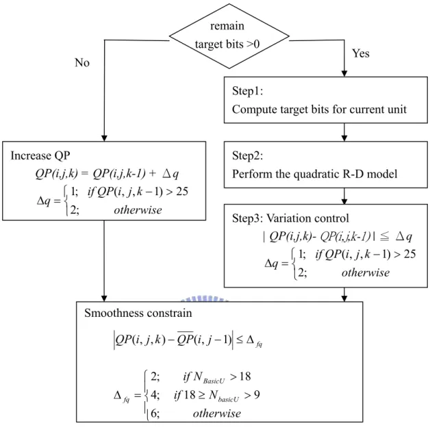
A basic unit is defined to be a group of continuous macroblocks, and the number of MBs in a basic unit is assigned by user. If the number of MBs in a basic unit is equal to 1, than it becomes a macroblock level rate control. In the H.264 rate control scheme, I-frame and B-frame is coded by one QP for entire frame, so the basic level rate control is only applied for P-frames. The block diagram of the basic unit level rate control is as follows:

remain target bits >0

Figure 2. Rate control flow chart

Step one allocates target bits to each macroblock according to the coding complexity. Tr(i, j) denote the number of remaining bits for the current encoding

frame, and its initial value is T0(i, j). The bit allocation for the current basic unit is

computed by Eq. (24).

∑

= × = basicU N k m estimate estimate r BasicU m j i MAD k j i MAD j i T k j i T ) , , ( ) , , ( ) , ( ) , , ( 2 2 , (24)

where NBasicU is the number of basic unit in a frame.

Step1:

Compute target bits for current unit Yes

No

Step2:

Perform the quadratic R-D model

Smoothness constrain fq j i QP k j i QP(, , )− (, −1) ≤∆ ⎪ ⎩ ⎪ ⎨ ⎧ > ≥ > = ∆ otherwise N if N if basicU BasicU fq 18 9 18 ; 6 ; 4 ; 2 Increase QP QP(i,j,k) = QP(i,j,k-1) + Δq otherwise k j i QP if q (, , 1) 25 ; 2 ; 1 − > ⎩ ⎨ ⎧ = ∆

Step3: Variation control

| QP(i,j,k)- QP(i,j,k-1) | ≦ Δq otherwise k j i QP if q (, , 1) 25 ; 2 ; 1 − > ⎩ ⎨ ⎧ = ∆

Step two computes quantization step by the quadratic rate distortion model in Eq. (20). Again, there are some constraints for ∆QP in order to ensure the smoothness of the visual quality. If it uses up target bits for current frame before it finishes encoding all macroblocks, the QP increases for encoding remain MBs.

3.4. Contrast Sensitivity Function Analysis

The HVS model tries to characterize the low-level processing functions of the visual systems, such as the optics, retina and striate cortex. These visual processes impose some limit on human visual capabilities. The Contrast Sensitivity Function (CSF) describes how sensitive the visual system is to the various frequencies of visual stimuli. For example, if the frequency of visual stimuli is too high, human will not be able to recognize the stimuli pattern any more. Many researchers proposed different forms of contrast sensitivity function [1][2][3][23], which will be investigated in this section.

In Ahumada CSF[23],the images are first converted to contrast images by subtracting and then dividing by the mean luminance of the background image. The method proposed by Mannos and Sakrison [1] has similar initial step that normalize all luminance values by the mean luminance. In HVS, visual sensitivity and perception of lightness are nonlinear functions of luminance. The amplitude of sensitivity is formulated as a nonlinear function of luminance level. In [1] [23], each pixel has global effect in the normalization step by using the mean luminance of the image. In Daly’s model[2], each pixel is transformed into a nonlinear-retinal-response value by Eq. (25) as follows:

63 . 0 ) , ( 6 . 12 ) , ( ) , ( ) , ( j i L j i L j i L j i L_r + = ₍₂₅₎

In the normalization step of Mannos-Sakrison CSF [1], the aspect of the visual system’s nonlinearity is characterized by cube root. This is a logical step since the eyes are known to be more sensitive to small variation in dark surroundings than in light ones. The normalization step in Mannos and Sakrison’s method is defined as follows: 333 . 0 ) , ( ) , ( _⎟⎟ ⎠ ⎞ ⎜⎜ ⎝ ⎛ = mean r _L j i L j i L (26)

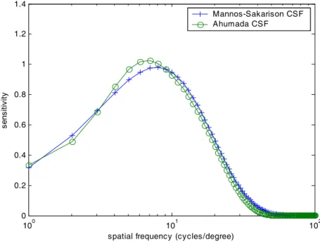
Each CSF model has slightly different features to model the sensitivity of human eyes to visual inputs of different spatial frequencies. Because the CSF is like a bandpass filter, many of the proposed function are composed of a high frequency lobe minus a low frequency lobe. Although it is known that the human visual system is not isotropic, most methods are simplified for easy implementation by minimizing the number of parameters. For this reason, the Mannos-Sakrison CSF and the Ahumada CSF are isotropic in frequency domain. Eq. (27) defines the transform from a Cartesian coordinate domain to an isotropic coordinate domain:

2 2 ), ( ) , (u v CSF r r u v CSF = = + . (27) (28)

Now, the Mannos-Sakrison CSF is defined in Eq. (28):

(

0.0192 0.144

)

exp( (0.144 ) ) 6 . 2 ) (_{r r r} 1.1 CSF_MS = + − .

⎟ ⎟ ⎠ ⎞ ⎜ ⎜ ⎝ ⎛ ⎟⎟ ⎠ ⎞ ⎜⎜ ⎝ ⎛ − − ⎟ ⎟ ⎠ ⎞ ⎜ ⎜ ⎝ ⎛ ⎟⎟ ⎠ ⎞ ⎜⎜ ⎝ ⎛ − = 2 2 exp exp ) ( s s c c Ah f r a f r a r CSF , (29)

where ac and as are the center and surrounding amplitude parameters, and fc and fs are

the center and surrounding cutoff frequency. In [23], they set a c =15.5, as/ac = 0.77,

fc = 20.8, and fc/fs = 5.6. In order to compare the Ahumada CSF with the

Mannos-Sakrison CSF, we modify the center amplitude ac to 1.176. From the

following figure, we can conclude that these two CSFs are very similar.

100 101 102 0 0.2 0.4 0.6 0.8 1 1.2 1.4

spatial frequency (cycles/degree)

se ns itiv ity Mannos-Sakarison CSF Ahumada CSF

Figure 3. The Mannos-Sakarison CSF and the Ahumada CSF

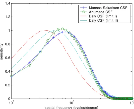
The Daly CSF is a function of many parameters, including radial spatial frequency, orientation, light adaptation level, image size in visual degree, and lens accommodation due to distance. Daly’s function is very complicated and Rushmeier et al. [3] rewrote a simplified version of Daly CSF which considers the radial spatial frequency parameter only.

(

0.3

)

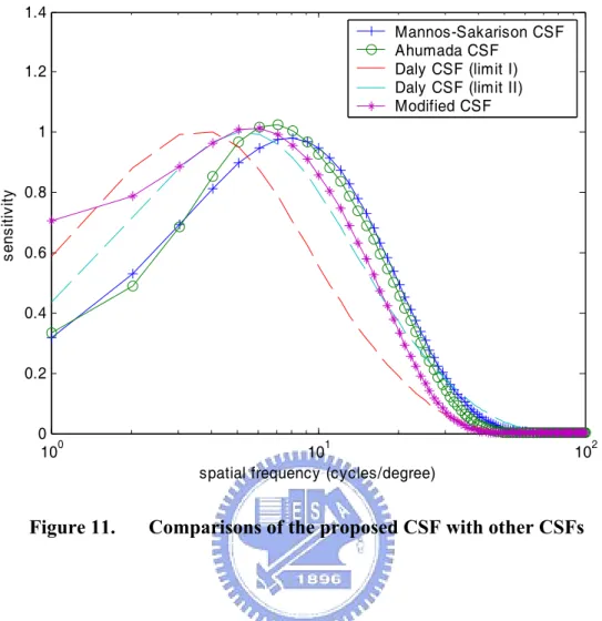
1 0.06exp(0.3 ) exp 42 . 1 1 008 . 0 0.2 3 r r r r CSF_DR ⎟ − + ⎠ ⎞ ⎜ ⎝ ⎛ ₊ = − (30)

The simplified function is showed as the Daly CSF (limit I) in Figure 4. The Daly CSF (limit II) in Figure 4 presents another sensitivity function for different orientation in the same viewing distance as Daly CSF (limit I). The figure shows that all the functions are close in performing the decreasing sensitivity in high frequency. In the next chapter, we will use this characteristics of CSFs to derive an new model for video rate control.

100 101 102 0 0.2 0.4 0.6 0.8 1 1.2 1.4

spatial frequency (cycles/degree)

se ns itiv ity Mannos-Sakarison CSF Ahumada CSF Daly CSF (limit I) Daly CSF (limit II)

Figure 4. Comparisons of four different CSFs

3.5. Perceptual-Based Objective Video Quality Assessment

The most common objective quality assessment method for image/video is the mean square error (MSE) and the peak signal-to-noise ratio (PSNR). These methods

are easy to compute and widely used in image/video research. However, the value of PSNR does not completely agree with the perceptual quality evaluated by human eyes. In order to develop a quality assessment that is consistent with human perception, many researchers proposed objective perceptual quality assessment with error sensitivity-based model, but most of them include complex computations.

Z. Wang et al. [24] proposed a measurement of structural distortion called structural similarity index (SSIM) to approximate the perceived image distortion. This model is based on the observation that the main function of the human visual system is to extract structural information, and HVS is highly adapted for this purpose. The proposed algorithm evaluates luminance, contrast and structural distortion separately first, and then combine these three measurements. Let x and y be two input images for evaluation. The luminance, contrast, and structure comparison measures are defined as follows: y x xy y x y x y x y x y x s y x c y x l σ σ σ σ σ σ σ µ µ µ µ = + = + = 2 , ( , ) 2 , ( , ) ) , ( _{2 2 2 2} , (31)

where µx, µy, σx2, and σy2 are the sample mean of x, the sample mean of y, the sample

variance of x, and the sample variance of y, respectively. And σxy is the sample

covariance of x and y defined as follows:

(

)(

)

∑

= − − − = N i i i xy x x y y N 1 1 1 σ . (32)

In luminance comparison, the form of µy can be written in the ratio of the mean luminance of x to the mean luminance of y and Eq. (31) can be rewritten as Eq. (33).

2 1 2 ) 1 ( 1 ) 1 ( 2 ) , ( , ) 1 ( x x y _C R R y x l R µ µ µ + + + + = + = . (33)

)

If C1 is small enough, then luminance comparison only relates to the proportion of µy

to µx . Therefore, this function is consistent with the HVS property that the influence

of relative luminance change is more major than the absolute luminance change. The similarity index measure S(x, y) between x and y is defined in Eq. (34):

(

2 2

)(

2 2 4 ) , ( ) , ( ) , ( ) , ( y x y x xy y x y x s y x c y x l y x S σ σ µ µ σ µ µ + + = ⋅ ⋅ = . (34)

)

To prevent unstable results when (µx2+µy2) or (σx2+σy2) is close to zero, the SSIM is

modified as follows:

(

)(

2 2 2 1 2 2 2 1)(2 ) 2 ( ) , ( C C C C y x SSIM y x y x xy y x + + + + + + = σ σ µ µ σ µ µ (35)

C1 and C2 are constants which are set to 6.5 and 58.5, respectively. The range of SSIM

is between 0 and 1. When input images x and y are identical, SSIM equal to 1. SSIM is computed for every pixel by using a sliding window. The window size is suggested to be 8×8. The quality of the entire image is the average SSIM of all pixels of the image.

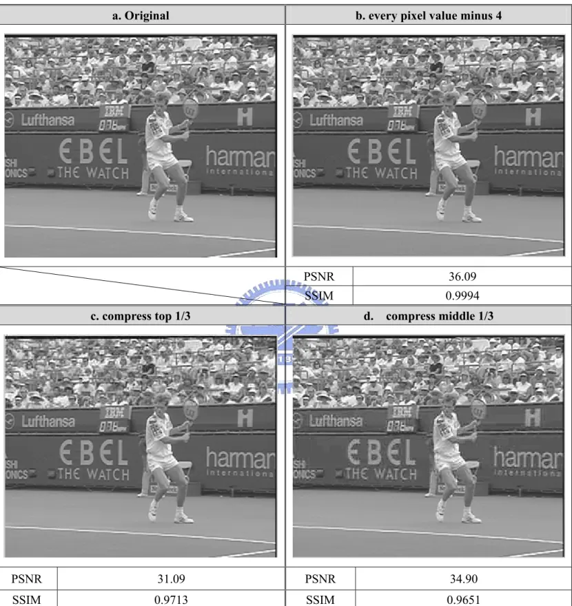
In the following experimental results, we can see the performance of image quality assessment using SSIM index compared to that using PSNR. In Figure 5(b) the luminance of entire frame is decreased by four gray levels, and this image looks almost the same as the original image Figure 5 (a). The SSIM value of Figure 5(b) is 0.9994, which means it is very similar to the original one. On the other hand, the

PSNR of Figure 5 (b) is only 36.09, which typically means it has noticeable distortions (usually, human vision sees distortions if an image has PSNR below 38). Figure 5(c) is composed of a JPEG compressed image on the top 1/3 of the image and the original image on the bottom 2/3 of the image, and Figure 5(d) is composed of JPEG compressed image in the middle 1/3 and the original image on the rest of the image. The distortion of the ‘audience’ area is less visible than the distortion of the middle part of this image. It is quite obvious that Figure 5(c) has better perceptual quality than Figure 5(d). However, the PSNR of Figure 5(c) and (d) are 31.09 and 34.90, respectively. This clearly shows that PSNR does not conform to human perceptual quality. On the other hand, the SSIM are 0.9713 and 0.9651 respectively. In this example, SSIM is more consistent with visual quality.

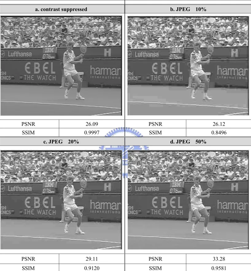
Figure 6(a) is processed with global contrast suppressed distortion, and Figure 6(b) is a JPEG compressed image with PSNR 26.12. These two images have similar PSNR, but have great differences in visual perception quality. The SSIM index of Figure 6(a) and (b) are 0.9997 and 0.8496 respectively. Obviously, SSIM can capture the prominent differences between these two kinds of images. Figure 6(b), (c), (d) and Figure 7 (a), (b) are JPEG images with different distortion levels. In Figure 6(b) and (c), the distortion, like blocking artifact and ringing artifact, is quite visible and the quality of image is poor. But it still can clearly discriminate that (c) has better quality than (b). Figure 7(a) has higher PSNR than Figure 6(b), but these two pictures are very close to the original image by visual assessment. The results on JPEG images are summarized in Table 1, where the increasing magnitudes of SSIM from low quality to high quality shows that it is more consistent with the degree of perceptual quality assessment.

a. Original b. every pixel value minus 4

PSNR 36.09 SSIM 0.9994

c. compress top 1/3 d. compress middle 1/3

PSNR 31.09 PSNR 34.90 SSIM 0.9713 SSIM 0.9651

a. contrast suppressed b. JPEG 10% PSNR 26.09 PSNR 26.12 SSIM 0.9997 SSIM 0.8496 c. JPEG 20% d. JPEG 50% PSNR 29.11 PSNR 33.28 SSIM 0.9120 SSIM 0.9581

a. JPEG 80% b. JPEG 95%

PSNR 37.75 PSNR 45.56 SSIM 0.9811 SSIM 0.9946

Figure 7. Comparison between SSIM and PSNR on high quality JPEG images

JPEG 10% JPEG 20% JPEG 50% JPEG 80% JPEG 95% PSNR 26.12 29.11 33.28 37.75 45.56 SSIM 0.8496 0.9120 0.9581 0.9811 0.9946

difference

PSNR 2.990 4.170 4.470 7.810 SSIM 0.0624 0.0461 0.023 0.0135

4. Proposed Rate Control Framework

In order to design the perceptual rate control model, we must first design a video complexity measure that can capture both the “coding entropy” and the “visual entropy” of video data. In another words, the distortion measure of the R-D model of a perceptual-based bit allocation algorithm must be based on a visual distortion measure. In our design, the video complexity measure is composed of the visual complexity term and the coding complexity term. The proposed measure is independent to video codec methods and can be used as a drop-in replacement of the SAD-based complexity model for any conventional rate control algorithms.

The organization of this chapter is as follows. First, section 4.1 describes the general requirement of a video complexity measure. Then, the visual complexity based on human visual system property is derived in section 4.2. Finally, the proposed perceptual model-based rate control scheme is presented in section 4.3.

4.1. Investigation of Video Complexity Measures

An image or a video frame is a projection of the three-dimensional (3-D) scene onto a two-dimensional (2-D) light-sensing surface, such as a photographic film or the photoreceptors of a human eye. Each pixel of the image represents the amount of light fell on the surface at a particular spatial position and at a particular time. When an object moves in the 3-D scene, the position of the object’s 2-D projection on the light-sensing surface changes correspondingly.

In psychological research, it is noted that one of the most important visual cues is the pattern of local retinal image velocity [33]. Therefore, the understanding and analysis of local motion information is crucial for video processing applications such

as video compression. The movement of the projected position of each point can be estimated from the spatiotemporal pattern of image brightness. Solving optical flow equation is the most commonly used method to estimate the local motion vectors at each image point. The optical flow equation assumes that the brightness of a projected 2-D image point remains constant over time regardless of whether the corresponding 3-D scene point moves or not [25]. Let the image brightness at the image position (x, y) at time t be denoted by I(x, y, t). The brightness of a particular point is constant, so that 0 = dt dI . (36)

By Taylor series expansion, Eq. (36) becomes:

ω + ∂ ∂ ∆ + ∂ ∂ ∆ + ∂ ∂ ∆ + = t I t y I y x I x t y x I t y x I( , , ) ( , , ) , (37)

where ω contains second and higher order terms. By subtracting I(x, y, t) from both sides and dividing by ∆t, we have:

0 ) (∆ = + ∂ ∂ + ∂ ∂ ∆ ∆ + ∂ ∂ ∆ ∆ t O t I y I t y x I t x . (38)

Taking the limit as ∆t→0, Eq. (38) becomes:

0 = ∂ ∂ + ∂ ∂ + ∂ ∂ t I y I dt dy x I dt dx , (39)

where ∂I/∂x,∂I/∂y are spatial partial derivatives, and ∂ /I ∂t is temporal derivation.

Usually, we let dt dy v dt dx u= , = , (40)

and (u, v) is the called the optical flow of I(x, y, t).

By our definition, visual complexity of video data represents how easy the HVS can discern any distortions in the data. Since local motions in the images is an important visual cue, from Eq. (39), we have a conjecture that both spatial partial derivatives and temporal partial derivatives of the image intensity function have large influence on visual complexity.

On the other hand, the coding complexity of video data characterize how well the prediction, transform, and quantization processes of a video codec can reduce the entropy of the data unit to be compressed. Conventional rate control algorithms uses SAD or MAD as an estimate of coding complexity.

Rate control involves adjusting quantization parameter in order to maintain the target output bitrate and minimizing overall distortion of the entire sequence. A general rate control model for H.264 was described in chapter 3.3. A rate control scheme generally includes two steps: (1) allocating target bits for a data unit, (2) using a rate-distortion model and given parameters, such as target bits and coding complexity to estimate suitable quantization parameter. In the basic unit level rate control, the first step (Eq. (24)) is calculated based on the MAD of the residual frame as coding complexity. The distribution of bit budget is proportional to the square of MAD. In the second step, it has to solve Eq. (20) for QP. Generally specking, the estimated QP is in direct proportion to coding complexity (e.g. MAD).

first order approximation of the local temporal derivatives of the video frame alone the motion trajectory. In another words, after removal of the “global” motion information of a video frame by the ME algorithm, the residual image is equivalent to the temporal derivative term in the optical flow equation (Eq. (39)). Since MAD is the average of a block of residual pixels, it can be considered as an indication of the magnitude of the optical flow (local motion) of the block. However, it does not tell you how “random” the local motion is.

As pointed out in [27], image pixels which can be tracked accurately by the eyes can have a stable projection on the retina and are visually more discernable. Therefore, a rate control algorithm based on MAD alone does not take into account the crucial visual information of local motion randomness. Furthermore, the existing rate control models do not consider the influence of spatial derivatives either. Spatial derivatives, in addition to being an important visual cue to local motion, are also related to spatial frequencies of the texture data. In the next section, we will present how these information can be used to construct a visual complexity measure.

4.2. Analysis of Visual Complexity

In the previous section, we postulate that visual complexity should be a function of both spatial partial derivatives and temporal partial derivatives. In this section, we will look deeper into spatial derivatives and its connection to the CSFs. Then, a visual complexity measure will be derived.

4.2.1. Relations between Spatial Derivatives and Filtering

From the Taylor’s series expansion, the first order derivative of a function f can be defined as the forward difference:

) ( ) 1 (x f x f x f _{= + −} ∂ ∂ . (41)

The result of this derivative is zero in the flat area and nonzero along the ramp. The second order derivative of function f can be defined similarly:

) ( 2 ) 1 ( ) 1 ( 2 2 x f x f x f x f _{= + + − −} ∂ ∂ . (42)

The result of this second order derivative is zero in the flat area and along ramps of constant slope, and is nonzero at start point and end point of a ramp. Notice that taking the image differences enhances discontinuities, such as the edge and the noise, and de-emphasizes the flat area with slowly varying gray levels.

In image processing applications, the isotropic filter (rotationally invariant filter) attracts much attention because the response of an isotropic filter is independent of the direction of the discontinuities. The simplest isotropic derivative operator is the Laplacian operator, which is defined as follows:

2 2 2 2 2 y f x f f ∂ ∂ + ∂ ∂ = ∇ . (43)

Eq. (43) is defined for function f with two parameters. The Laplacian of any order is a linear operator. The second order partial derivative in x-direction can be computed by:

) , ( 2 ) , 1 ( ) , 1 ( 2 2 y x f y x f y x f x f _{= + + − −} ∂ ∂ . (44)

Similarly, the second order partial derivative in y-direction is computed by:

) , ( 2 ) 1 , ( ) 1 , ( 2 2 y x f y x f y x f y f _{= + + − −} ∂ ∂ . (45) (46) Equation (43) becomes: ) , ( 4 ) 1 , ( ) 1 , ( ) , 1 ( ) , 1 ( 2_{f = f x+ y + f x− y + f x y+ + f x y− − f x y} ∇

Eq. (46) can be implemented by the convolutional masks in Figure 8. It also can incorporate the diagonal direction in the definition of Laplacian function and the mask (shown in Figure 8 b).

(a) (b) (c) (d)

Figure 8. Laplacian masks

The resulting images after applying Laplacian kernels has edge lines and other discontinuity like noise point.

It is well known that Fourier transform takes a function in the time domain into the frequency domain. It decomposes a function into harmonics of different frequencies. Therefore, there certainly exist a filter in frequency domain corresponding to a filter mask in spatial domain. It is generally more intuitive and computationally more efficient to perform the filtering in frequency domain.

A smoothing spatial filter mask and the filter function are shown in Figure 9. The corresponding filter in frequency domain is a lowpass filter. Low frequencies in the Fourier transform represents smooth area, while high frequencies in the Fourier transform rpresents derail features, such as edge and noise. The mask is the operator to compute the spatial derivatives. The corresponding filter in frequency domain is a highpess filter. A highpass-filtered image would emphasize detail areas and suppress the gray level variation in smooth place. The illustrations in Figure 9 indicate that the operations of the small filter mask in spatial domain and the corresponding filter in frequency domain are the same.

Figure 9. Filters in different domain [38]

4.2.2. Spatial Contrast Sensitivity

Human visual system has different sensitivity to different spatial frequencies, and the operation is like a lowpass or slightly bandpass filter. The contrast sensitivity function describes the sensitivity of HVS to different frequencies. Based on numerous experiments [34], the peak frequency in a CSF is generally between 3 cycles/degree and 8 cycles/degree, and the sensitivity in high frequencies data decreases rapidly. When a CSF filter is applied to an image, a portion of high frequency information that

is not detectable by human visual system would be filtered out. The filtered information can be used to estimate the visual complexity of the video data.

The process of how CSF can be applied to an image is presented in [1]. The first step is to normalize all luminance values in the image by the mean luminance. Because visual perception of lightness is a nonlinear function of luminance, the cube root of the normalized luminance is taken over the entire image. Since a CSF is easier to describe in frequency domain, the Fourier transform F(u, v) of the image f is computed first. The signals in frequency domain are then filtered by a CSF as follows:

)) , ( ( ) , ( ) , (u v F u v CSF r u v G = ⋅ . (47)

The inverse Fourier transform of G(u, v) is the filtered image.

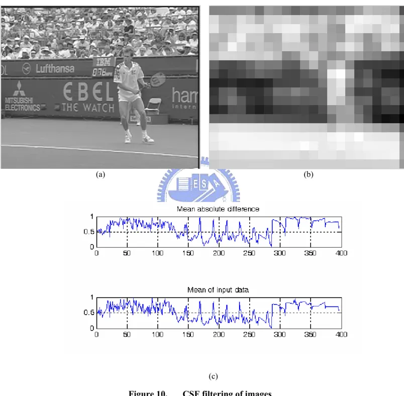
In most applications of CSF, it is used for quality assessment by computing the difference between the two CSF-filtered input images. For video coding purposes, we are more concerned about the amount of data which is filtered out by the CSF. An area with lots of filtered data means that there is more visually undetectable information. Therefore, the amount of filtered information is estimated by computing the absolute difference between images before and after the filtering process. The estimation of visual complexity will be incorporated into the rate control of video compression. Since the smallest coding unit for rate control is a macroblock, the filtered information will be computed on a macroblock basis. MAD is computed to evaluate the average amount of the dropped data. The area with more data dropped is less important. However, the evaluated result is highly correlated to the original luminance and not accurate. Figure 10 illustrates this phenomenon. Figure 10(a) is the original frame from the Stefan sequence. Figure 10(b) is the MAD that represents the merged information for one macroblock. It is quite obvious that the result is similar to the