基於EEMD與類神經網路建構台指期貨交易策略 - 政大學術集成

全文

(1)國立政治大學理學院應用物理研究所碩士論文 Graduate Institute of Applied Physics, College of Science National ChengChi University Master Thesis. 政治大. 基於 EEMD 與類神經網路建構台指期貨交易策略立. ‧. ‧ 國. 學. A study of Trading Strategies of TAIEX Futures by. y. Nat. n. al. er. io. sit. using EEMD-based Neural Network Learning Paradigms. C h 陳原孝 engchi. i n U. v. Chen Yuan Hsiao. 指導教授：蕭又新博士 Advisor: Shiau You Hsien, Ph.D.. 中華民國 102 年 1 月 January, 2013 1.

(2) 摘. 要. 金融市場瞬息萬變，股價漲跌似乎沒有顯著的規則，這意味著股價的行為特徵是不可精確預知和不確定的，為了在市場上增加收益和減少投資風險，研究人員不得不試圖建立一個有效預測金融市場的模型，它可以估算這種不確定性的影響，很可惜的，至今仍然沒有一個模型接近成功的。沒有成功的模型並不代表它是不存在的，相反的，研究人員需要建立更多的預測模型，以提供市場判斷的經驗法則。我們使用 ARMA 與兩種不同形式的 EEMD-ANN 去對台灣加權指數期貨做預測值. 政治大場之價格後，我們使用 2 立種交易策略去做績效測試，本研究希望能夠找到較適合的精確度比較，我們比較了兩種不同的行情：趨勢與震盪。此外，預測出未來市. ‧ 國. 學. 使用在指數預測的預測模型。. 另外在本文中，我們也分析影響 TAIEX 價格波動的因素，透過 EEMD，我們可. ‧. 以將其拆解成數具有不同物理意義的本徵模態函數(IMF)，再藉由統計值選出較. n. al. er. io. sit. y. Nat. 重要的 IMF 並分析其意義。. Ch. engchi. i n U. v. 關鍵字:總體經驗模態、類神經網路、自回歸移動平均模型、交易策略、預測模型 2.

(3) Abstract Financial market changes constantly and Stock Price Volatility (SPV) seems to be no significant rules. This means behavioral characteristic of the stock price cannot foresee and uncertain accurately. In order to increase revenue and reduce investment risk in the market, researchers had to try to establish an effective prediction model of financial markets. It can estimate the impact of this uncertainty. It's a great pity that there is not a model that is close successfully yet. That does not represent it does not exist successful model. Instead, researchers need to establish more predictive models. 政治大 The forecasting results of 立TAIEX Index futures by ARMA Model and two types of. to offer the market to judge the rule of thumb.. ‧ 國. 學. EEMD-ANN Models were compared in two kinds of markets – trend and fluctuation. In addition, two trading strategies were tested after the future prices are forecasted.. ‧. The study attempted to identify a suitable forecasting model.. Nat. sit. y. Moreover, the factors for price fluctuation of TAIEX were also analyzed in the. n. al. er. io. study. Through EEMD, they could be decomposed to IMFs with various physical. i n U. v. meanings and more important IMFs were selected to be analyzed in accordance with the statistic value.. Ch. engchi. Keywords: Ensemble Empirical Mode Decomposition, Artificial Neural Network, ARMA, Trading strategy, Forecasting model 3.

(4) List of Contents 摘要................................................................................................................................... 2 Abstract ............................................................................................................................. 3 List of Contents ................................................................................................................. 4 List of Pictures .................................................................................................................. 5 List of Tables..................................................................................................................... 6 Chapter 1. Introduction ................................................................................................. 8. Chapter 2. Methodology ............................................................................................. 13. 政治大 2.2 Ensemble Empirical Mode Decomposition (EEMD) ....................................... 17 立. 2.1 Empirical Mode Decomposition (EMD) .......................................................... 13. 2.3 Artificial Neural Networks (ANNs) .................................................................. 19. ‧ 國. 學. 2.4 EEMD-based neural network learning paradigm.............................................. 24. Experimental Details ................................................................................. 26. sit. y. Nat. Chapter 3. ‧. 2.5 ARMA Model.................................................................................................... 25. io. er. 3.1 Data description ................................................................................................ 26 3.2 The Operation of Price ...................................................................................... 29. al. n. v i n Ch 3.3 Statistical measures ......................................................................................... 31 engchi U. 3.3 Significant IMFs ............................................................................................... 33 3.4 Experiment design............................................................................................. 49 3.5 Performance .................................................................................................... 54 Chapter 4. Algorithmic Trading .................................................................................. 61. 4.1 Trading Strategy I ............................................................................................. 61 4.2 Trading Strategy II ............................................................................................ 67 Chapter 5. Conclusion................................................................................................. 72. References ....................................................................................................................... 73 4.

(5) List of Tables Table 3.1 the Trading Volumes from 2000 to 2005......................................................... 27 Table 3.2 the Trading Volumes from 2006 to 2011 ......................................................... 27 Table 3.3 the Specification for TAIEX Futures............................................................... 28 Table 3.4 the Statistical Measures of the Components Decomposed from TAIEX Index................................................................................................................................ 36 Table 3.5 the Statistical Measures of each term Combined from the TAIEX Index Components .................................................................................................................... 37. 政治大 Other Investors ................................................................................................................ 39 立 Table 3.6 the Statistical Measures of each term from the Trading Value of Foreign &. Table 3.7 The Correlation Coefficients Compared the Trading Value of Foreign &. ‧ 國. 學. Other Investors with TAIEX Index in terms of High Frequency .................................... 40. ‧. Table 3.8 Incidents .......................................................................................................... 43. sit. y. Nat. Table 3.9 the Correlation Coefficients Compared Leading indicator with TAIEX Index. io. er. in terms of Low Frequency ............................................................................................. 46 Table 3.10 the Correlation Coefficients Compared Real GDP with TAIEX index in. al. n. v i n Ch terms of Trend ................................................................................................................. 48 engchi U Table 3.11 the Example of TAIEX Futures ..................................................................... 55 Table 3.12 the Forecasting Accuracy for the First Half Year .......................................... 58 Table 3.13 the Forecasting Accuracy for the Latter Half Year........................................ 59 Table 3.14 Average Fluctuation Range for Each Month ................................................. 60 Table 4.1 the Correct Trend (%) of Every Month ........................................................... 62 Table 4.2 the Profit of Trading Strategy I in 2010 .......................................................... 64 Table 4.3 the Profit of Trading Strategy II in 2010 ......................................................... 71. 5.

(6) List of Figures Figure 2.1 the Flow Chart of EMD ................................................................................. 16 Figure 2.2 Three-Layer Neural Networks ....................................................................... 20 Figure 2.3 the Structure Chart of BPNN‘s Training Progress......................................... 22 Figure 2.4 A Fully Connected with Four-Layer Feed- forward Network ........................ 23 Figure 3.1 the Booming Figure of Trading Volumes during 2000 ~2011 ....................... 27 Figure 3.2 the TAIEX Futures during 2010 .................................................................... 29 Figure 3.3 the TAIEX Index from 2004 April to 2012 July ............................................ 35. 政治大 Figure 3.5 the Four Terms Combined 立 from the TAIEX Index Components................... 37 Figure 3.4 the IMF1~ IMF5 and the Residue Decomposed from TAIEX Index ............ 35. ‧ 國. 學. Figure 3.6 the IMF1~ IMF5 and the Residue Decomposed from the Trading Value of Foreign & Other Investors .............................................................................................. 38. ‧. Figure 3.7 the Relative High Point and Low Point ......................................................... 40. Nat. sit. y. Figure 3.8 the January Effect .......................................................................................... 42. n. al. er. io. Figure 3.9 the Big Events................................................................................................ 43. i n U. v. Figure 3.10 Business Cycle............................................................................................. 44. Ch. engchi. Figure 3.11 Low Frequency term from 2004 April to 2012 July .................................... 45 Figure 3.12 Leading indicator from 2004 April to 2012 July ......................................... 45 Figure 3.13 the Comparisons between GDP and Trend from 2004 to 2012 ................... 47 Figure 3.14 Comparisons between GDP and Trend from 1991 to 2011 ......................... 48 Figure 3.15 Flow Chart of EEMD-ANN Model 1 .......................................................... 50 Figure 3.16 Flow Chart of EEMD-ANN Model 2 .......................................................... 51 Figure 3.17 Training Network by Moving Window Process (Model 1) ......................... 52 Figure 3.18 Training Network by Moving Window Process (Model 2) ......................... 53 Figure 3.19 the Shape of a Candlestick .......................................................................... 54 6.

(7) Figure 3.20 Trade Success .............................................................................................. 55 Figure 3.21 Trade Failure................................................................................................ 56 Figure 3.21 Fluctuations from January to June............................................................... 57 Figure 3.21 Trends from July to December .................................................................... 57 Figure 4.1 the Trading Chart of 2010 September ........................................................... 63 Figure 4.2 Forecast of Price Dropping on 2010/2/6 (Model 1) ...................................... 66 Figure 4.3 Forecast of Price Rising on 2010/2/6 (ARMA)............................................. 66 Figure 4.4 Bull and Bear Market .................................................................................... 68. 政治大 Figure 4.4 the Second Stop- loss Method ........................................................................ 70 立 Figure 4.4 the First Stop- loss Method............................................................................. 69. ‧. ‧ 國. 學. n. er. io. sit. y. Nat. al. Ch. engchi. 7. i n U. v.

(8) Chapter 1 Introduction. Today‘s world is undergoing tremendous changes. Digital virtual world made by Web have dominated human civilization in decades. Explosive increase therefore occurs in the degree of social complexity and the rate of trend changes. Some researchers consider that no one is able to predict great events or trends after the next presidential election or reformulations in Federal Reserve System in this kind of gradual complex and continual varied world. However, some researchers think that. 政治大 the cycles of events despite the fact that life is getting complex. So far, there are more 立 we are more capable to predict because the advanced technology make us understand. and more researchers who support the later concept. In ―The Great Depression. ‧ 國. 學. Ahead―, which was written by American notable economist and predictor Harry S.. ‧. Dent Jr., said: ―Greater complexity leads to greater information and intelligence. y. Nat. (including technology and now computers) that actually allow greater predictability. er. io. sit. over time from the macro to the micro arenas. ‖ Moreover, EU establishes a computer system project called ―Living Earth Simulator Project.‖ This project uses the latest. al. n. v i n super computer to analyze greatC amount of information h e n g c h i Uin Social Networking Services and governmental statistics. They find the trends of human politics and economy, and. then take steps to prevent problems like epidemic or financial crisis. Similarly, prediction on stock price will be one of the popular researching fields in financial market as well. The financial market is a complex, evolutionary, and nonlinear dynamical system (Abu-Mostafa and Atiya, 1996). It is hard to discover regulations by using traditional time series predicting in high nonlinear dynamical system like stock market. This is also the greatest obstacle when researchers build predicting models. The models‘ consequences are wrong producing or wrong deciding plenty of financial crises. Fortunately, Artificial Neural Network (ANN) provides solutions to 8.

(9) nonlinear problems. ANN can abstract useful data among database. It is adaptively formed basing on the features presented in the data. In this study, we focus on the development of a stock market forecasting model based on artificial neural network architecture. This study constructs ARMA and two different EEMD-based ANN algorithm as a baseline model, which enables us to test the TAIEX index futures return. ANN has been successfully applied in financial fields. Hamid et al. (2004) compared volatility forecasts from neural networks with implied volatility from S&P. 政治大 futures options pricing model. Forecasts from neural networks outperform implied 立. 500 Index futures options using the Barone-Adesi and Whaley (BAW) American. volatility forecasts and were not found to be significantly different from realized. ‧ 國. 學. volatility. Implied volatility forecasts were found to be significantly different from. ‧. realized volatility in two of three forecast horizons.. sit. y. Nat. Lin and Yu (2009) transformed ANN prediction into a simple FK indicator for. io. er. decision making trading strategy, whose profitability was evaluated against a simple buy-hold strategy. They adopted the neural network approach to analyze the Taiwan. al. n. v i n C hin the States. Consequently, Weighted Index and the S&P 500 they found that the engchi U trading rule based on ANNs generated higher returns than the buy-hold strategy.. Jasemi et al. (2011) presented a model to do stock market timing on the basis of the TA of Japanese Candlestick and concept of Neural Networks with astonishing results. In this approach, the network was not going to learn the candlestick lines alone or in combination, but was to present a kind of regression model whose independent variables were important clues and factors of the technical analysis patterns; and its dependent variable was the market trend in near future. In defining the independent variables two approaches were taken; one was Raw data-based and the other is Signal-based with fifteen and twenty-four variables, respectively. Experimental results, 9.

(10) in which estimated signals are compared with actual events according to real published daily data in Yahoo, finance, showed that the proposed model performs brilliantly well in emission of buy and sell signals while the first approach seems to some extent better than the second. Yoon et al. (1991) used forth- layer Back-propagation Neural Network (BPNN) cataloging profits to companies‘ stock prices and predicts that whether the future performance on stock prices better or worse. He used confidence degree, economic factors, growth rate, and strategies to profit, new products, expected loss, expected. 政治大 variables in Input layer. He compared the consequences of this conducing way and 立 profit, long-term or short-term optimistic degree, and other professional estimable. statistic distinguishing analysis, both in-sample and out-sample results are better.. ‧ 國. 學. Ken-ichiKamijo and Tanigawa-Tetsuji (1990) used ANN to analyze K-line in. ‧. Tokyo Stock Exchange. They analyzed triangle patterns of K- line major to find the. sit. y. Nat. trend of price changes. After 15 training patterns learning, they used 16 testing. io. 16 experiments. The accuracy rate was high up to 93.8%.. n. al. Ch. Douglas Wood and Bhaskar.Dasqupta (1994). engchi. er. patterns to predict. The result in test triangle was accurately recognized in 15 out of. iv n used U ANN,. multiple regression. analysis, and ARINA predicting French capital market. They found ANN‘s accuracy rate is over 50%, and the others are less then it. Zheng-Hsiu Chu (2004) used multiple regression analysis, time series analysis and ANN to analyze 279 weekly trading data from 14 countries. The result was that the improved back propagation network was the best and then was multiple regression analysis in the predicting model return rate. The preceding historical examples are all applications of ANN in financial area. Recently, ANN also developed a predicting way that is different from traditional one. It is call EMD-ANN or EEMD-ANN. 10.

(11) En Tzu Li (2011) found EEMD-ANN Network which was more proper to use in predicting index and she did predicted the future index price. As a result, the FK value can display a signal if to buy or sell, and confirm trading time, and make buy or sell Call-Put decisions on TAIEX options. Lean Yu et al. (2008) used an EMD-based neural network ensemble learning paradigm for world crude oil spot price forecasting. In terms of empirical results, Yu find that across different forecasting models, for the two main crude oil prices – WTI crude oil spot price and Brent crude oil spot price – in terms of different criteria, the. 政治大 Lean Yu et al. (2010) proposed an EMD-based multi-scale neural network learning 立. EMD-based neural network ensemble learning model performs the best.. paradigm to predict financial crisis events for early- warning purposes. They used. ‧ 國. 學. EMD to decompose the important part of data. Using the neural network weights,. ‧. some important intrinsic mode components were selected as the final neural network. sit. y. Nat. inputs and some unimportant IMFs that were of little use in mapping from inputs to. io. er. output are discarded. Using these selected IMFs, a neural network learning paradigm was used to predict future financial crisis events, based upon some historical data.. al. n. v i n C hthe proposed multiUscale neural network learning Experimental results revealed that engchi. paradigm could significantly improve the generalization performance relative to conventional neural networks.. Tsai Yu Ching (2011) applied the Ensemble Empirical Mode Decomposition (EEMD) based Back-propagation Neural Network (BPNN) learning paradigm to two different topics for forecasting: the hourly electricity consumption in National Chengchi University and the historical daily gold price. They used moving-window method in the prediction process. Good accuracy was revealed after using the method and strategy in this prediction. Moreover, they used the ensemble average method, and compared the results with the data produced without applying the ensemble 11.

(12) average method. By using the ensemble average, the outcome was more precise with smaller errors. It resulted from the procedure of finding minimum error function in the BPNN training. The purpose of this study is to compare the accuracies of ARMA and EEMD-ANN Models and establish trading systems in accordance with the forecasting values. It was appropriate to define a clear price trend which allows us establish trading systems to enter or exit positions. We input the IMFs which is the effect of TAIEX futures to a back-propagation neural network (BPNN) to predict a clear price. The stock index. 政治大 spot in the future. So, we discussed factors (which affecting index) as well. 立. spot should be considered while trading the index futures since they are actually the. ‧. ‧ 國. 學. n. er. io. sit. y. Nat. al. Ch. engchi. 12. i n U. v.

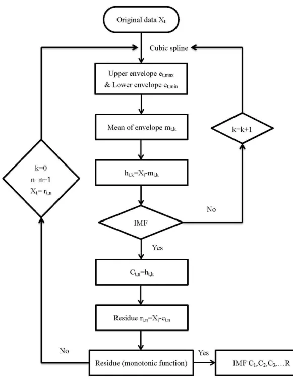
(13) Chapter2 Methodology. 2.1 Empirical Mode Decomposition (EMD) Empirical Mode Decomposition (EMD, Huang et al., 1998) is a novel method analyzing non-linear, non-stationary data. This method is based on local time scale, extracting intrinsic mode function from original data. It is applied by decomposing oscillation one by one of different time scale in the original data, producing a series of oscillatory mode from high frequency. 政治大 physical meanings. Each IMF means a component of time scale oscillation in original 立 to low frequency. Each scale represents an IMF. It makes IMF having obvious. Each IMF has to match the following two definitions:. 學. ‧ 國. data; while residue shows trend of them.. ‧. 1. The number of total local extrema (including local maxima and local minima) and. y. Nat. the number of zero-crossings must either equal or differ by at most one.. er. io. sit. 2. At any point, the mean value of the ―upper envelope‖ (determined by the local maxima) and the ―lower envelope‖ (determined by the local minima) is zero.. al. n. v i n The IMF decomposed by twoCdefinitions above is U h e n g c h i approximate mono-components. and signals which are almost orthogonal. However, there are a lot of natural data containing various frequencies. EMD uses a shifting process in order to find definition- matching IMF, symmetrize waveform, and ridding riding wave. Use EMD to decompose the data. The input data must satisfy the following three conditions: 1. There must be two extremes of the data: a maximum and a minimum. 2. Data characteristic time scale is defined as the time difference between the two extremes.. 3. If the data contains no extreme but inflection points, we do once or more times of 13.

(14) differential with the signal until finding the extreme. The final results can be obtained from integral component differential. Base on the establishment of the above conditions. The EMD sifting process is as follows: (1) Used a cubic spline lines to connect all maxima of the upper envelope et,max by the local maxima of the data Xt and local minimum value; The minimum value is connected to form the lower envelope et,min (2) The maximum value of the envelope plus minimal value envelope; Take the. 政治 e e 大 . average to obtain the mean envelope. 立. m. t,max. t ,k. t ,min. 2. h =X - m t,k. t. ‧. ‧ 國. get. 學. (3) The original data Xt by subtracting the mean envelope obtained component ht,k , we. t,k. y. Nat. io. sit. Judgment obtained component meets the IMF two definitions. If not, then ht,k is. n. al. er. repeated as the input. Step 1~3 continues shifting and filtering iterative procedure. i n U. v. when the obtained component satisfied with two definitions of IMF.. Ch. engchi. Let ht,k express into c t,n . It's expressed as follows:. c. t,n. =. h. t,k. Let the original signal Xt deduct IMF component, and then we can be obtained a residual rt,n. It's expressed as follows:. r =X -c t,n. t. t,n. And so on, IMF definition can be satisfied in order. Signal, Ct,1 ,Ct,2 ,Ct,3 ,…Cn, frequency gradually decreasing.. 14.

(15)  X t  c t ,1  r t ,1  c t ,2  r t ,2  r t ,2  c t ,3  r t ,3      r t ,n 1 c n r n rn is a monotonic function of the process. Until IMF can no longer be separated, the entire EMD decomposition process can be considered complete. rn is trend term in EMD decomposition process, and the original signal can be expressed as the sum of the IMF and the trend term. It's expressed as follow: n 1. X t   ci  r n. 政治大 i 1. 立. ‧ 國. Residue. 學. Set IMF. The shifting process automatically generates the value of the zero reference line for. ‧. each IMF. The data for a long-time trend term will be separated to rn independently. In. Nat. sit. y. order to avoid too much filtering to make IMF loss the physical meaning of the. n. al. i n U. shifting process, called the Standard deviation, SD values.. Ch. engchi. (ht ,k 1ht ,k ) 0.2  SD   h T. 2. t 0. er. io. original single-component signal, therefore joined stopping criterion to end the. v. 2.  0.3. t , k 1. SD is the amount of change between the two iterations of the component as a stop criterion. To stop filtering iterations action SD ranged from 0.2 to 0.3, and completed once the IMF's calculations. We can get the IMF by the high frequency to low frequency upon completion of the shifting process. Each IMF has physical meaning.. 15.

(16) 立. 政治大. ‧. ‧ 國. 學. n. er. io. sit. y. Nat. al. Ch. engchi. i n U. v. Figure 2.1 the Flow Chart of EMD. 16.

(17) 2.2 Ensemble Empirical Mode Decomposition (EEMD) It is really a very practical method that the EMD for nonlinear and non-stationary information. But there will be mode mixing problem in the process of empirical mode decomposition mixer wave. That is to say that there will be different signals mixed in the same intrinsic mode functions (IMF), or the same time scale signals appear in different intrinsic mode functions (IMF). This will reduce the physical significance of the IMF. For mixer wave, Wu and Huang (2004) proposed the Ensemble Empirical Mode Decomposition (EEMD) to overcome this problem. The EEMD modal. 政治大 noise decomposition performs an overall before pre-decomposition signal. In other 立 characteristics of white noise contain various frequency scales, adding random white. words, the original signal added random white noise, do EMD decomposition first,. ‧ 國. 學. and then averaging the results of the decomposition. So, the white noise uniformly. ‧. distributed in each component. The original signal will decompose to the appropriate. sit. y. Nat. frequency of component. Repeat the above steps, which are able to get more in line. io. er. with the actual conditions of the real results.. The statistical know that adding white noise caused the error between the original. al. n. v i n After a large number ofC statistical Wu et al. Empirical h e n g c h i U formula. signals.. . n. . is given:. . n. n is represents the number of ensemble members; ε is the amplitude of the added noise; εn is the final standard deviation of error defined as the difference between input data and the corresponding IMFs (standard deviation of error). In the implementation, we will modulation the two parameters εn and N. As εn increased, errors also become large. Other hand, sometimes the N value is insufficient and apt to cause the signal of the same frequency range decomposed into two signals. So it is very important to choose the appropriate averaging time. The number of the 17.

(18) ensemble numbers N is always set to 100 and the εn always set to 0.1 or 0.2 (Zhang et al., 2008) based on experience. The following is EEMD decomposing process: 1. Add a white Gaussian noise εt,i to the original data xt to create a new data. That is. y. t ,i. . x  t. t ,i. xt is original data , εt,i are different realizations of white Gaussian noise. 2. Use EMD to decompose each yt,i. You can get n IMF which can write as ct,ij and a residue rt,i. ct,ij means the number j IMF after adding i white noise.. 政治大. 3. Use ensemble average to the above IMFs. You can get the final IMF , which is:. 立. N. c. c. 1 t, j N i. t ,ij. ‧ 國. 學. ct,j means the j IMF after using EEMD decomposition to original signal. Through the above three steps, we already can get IMF more accurately and. ‧. meaningful. However, in applying, IMFs vary every time after EEMD decomposition.. y. Nat. sit. The reason is that EEMD adds different white Gaussian noise randomly. With the. n. al. er. io. differences of εn‘s number, the results vary to each other. Even one selects the same. i n U. v. parameter, the result is different. For example, εn simulates as 0.1, N simulates as 100,. Ch. engchi. the results are still different from each other. But after doing averages many times, the interferences of white Gaussian noise will turn small, which is near the real answer. In this study, we use EEMD to analyze TAIEX index, and get a series of meaningful IMF. We are trying to explain these affecting reasons.. 18.

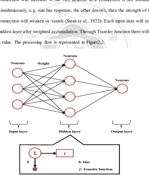
(19) 2.3. Artificial Neural Networks (ANNs) Artificial Neural Networks (ANNs) is an Artificial Intelligence Machine using mathematical method. And via computer ‘s rapid calculating ability, it makes computer have ability of predicting. It can simulate nonlinear function. After several times of simulations, ANN becomes a complex functional form. Therefore, it is suitable for solving complex questions of nonlinear system. Besides, one doesn‘t have to presupposition before using ANN. You can start analyzing just preparing enough history data. For instance, if one knows the factor of Fundamental information or. 政治大 experiments proves, ANN can be applied on many field which old computer system 立. Technical Information, he can use ANN to start stock index prediction. After many. cannot reaches, just as Face Recognition (Rowley et al., 1998)、Financial forecasting. ‧ 國. 學. (Gately, E., 1996)…etc. In addition, ANN has potential ability of predicting time. ‧. scale models and Nonparametric estimated as well (Kuan and White, 1994).. sit. y. Nat. This section gives an introduction to basic neural network architectures and. io. er. learning rules. An ANN‘s all Neurons are layered by their functions. Three layers in general: input layer, hidden layer, and output layer. Each layer is linked by foregoing. n. al. order.. Ch. engchi. i n U. v. 1. Input layer: use to represent input variable data. Neurons‘ number are depends on question. In this study, we use IMF decomposed by EEMD as input data. 2. Hidden layer: use to represent the inter-effects between input data. In many research results and engineering simulation all shows hidden layer doesn‘t need above two layers (Hush and Horne, 1993) , pointed out network which use two layers in hidden layer, each layer only has a few neurons. It can be replaced by a network with a great amount of neurons in a layer. Moreover, the amount of neurons has to use trail route to decide its best number. ANN 19.

(20) cannot depict the system properly with too little number of neurons. Too large number of neurons will provide over- fitting problem (I. Kaastra, M. Boyd, 1996). 3. Output layer: use to represent output data. In this study, we predict TAIEX futures price. Therefore, the neuron‘s number is 1 in output layer. The basic principle of ANN is using weight to connect each layer ‘s neurons. If there are two neurons is stimulated at once by a connection, the strength of this connection will increase. If the two neurons in a connection is not stimulated. 政治大 connection will weaken or vanish (Stent et al., 1973). Each input data will reach 立 simultaneously, e.g. one has response, the other doesn‘t, then the strength of this. a value. The processing flow is represented in Figure2.2.. 學. ‧ 國. hidden layer after weighted accumulation. Through Transfer function there will be. ‧. n. er. io. sit. y. Nat. al. Ch. engchi. i n U. Figure 2.2 Three-Layer Neural Networks 20. v.

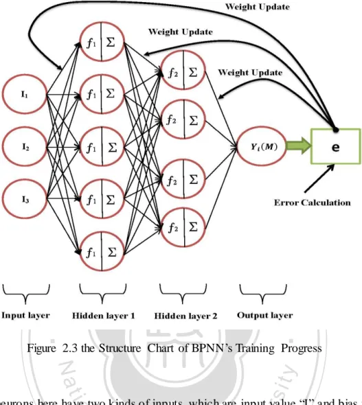
(21) Transfer functions are mathematical formulas that determine the output of processing neurons. The selection of transfer function will affect the whole network‘s trait. Therefore, networks having different characteristic have to select different transfer functions. Three kinds of transfer functions which are usually used in Back-Propagation Neural Network. in this paper is: hyperbolic function, log-sigmoid function and linear function. Hip( x) . e x  e x e x  e x. Sig ( x) . 1 1  ex. Lin( x)  x. 政治大. Since financial markets are nonlinear, nonlinear transfer functions are more favored.. 立. So far, In ANN applying, the most popular one is Back-Propagation Neural Network. ‧ 國. 學. (Rumelhart et al., 1986). It adopts the Widrow-Hoff learning rule (i.e. least mean squared (LMS) rule) (Hagan et al., 1996).The mean square error function could be. ‧ y. 1 N 1 N 2 M  [ ( )]  [  (M )]2 N i 1 e i N i 1 t i Y i. io. sit. Nat. F (M ) . er. presented as:. 𝑌𝑖 (𝑀) is the final output value, ti is the target value, and 𝑒𝑖 (𝑀) is the error between. al. n. v i n C h flow is represented 𝑌𝑖 (𝑀) and ti. The processing in Figure2.3. engchi U. the values. 21.

(22) 立. 政治大. ‧. ‧ 國. 學. Figure 2.3 the Structure Chart of BPNN‘s Training Progress. sit. y. Nat. n. al. er. io. The neurons here have two kinds of inputs, which are input value ―I‖ and bias value. i n U. v. ―b‖. ‖I‖ is the real input data. In this study, our input values are IMFs after EEMD. Ch. engchi. decomposition. They have to multiply the weights which connect hidden layer. ―b‖ is value which directly input in neurons. It is used to apply non-leaner Threshold Value. Therefore, the formula of ANN dynamical system which has M layers can be expressed as: for 1≤i≤ N m, 1≤j≤ N m, 1≤m ≤M. Y. m i.  N m m m 1  f   wij Y j  b i   f  j 1 . n  m. i. Each ANN contains Nm neuron and the iteration calculation is able to reflect one layer of the process unit in the network. For instance, the neuron i on the layer m accepts all the processed and weighted inputs from (m-1) layer and then adds external 22.

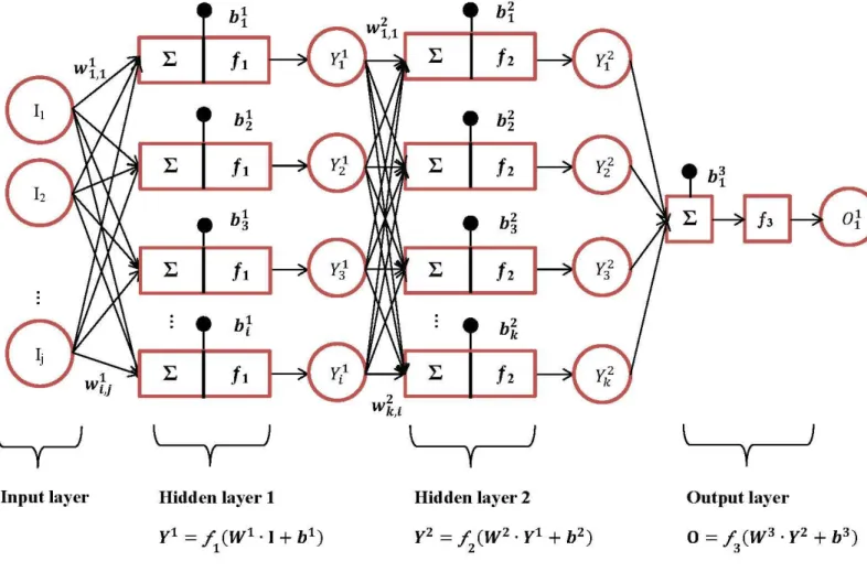
(23) input of. 𝑖. to produce. 𝑖. . 𝑌𝑖. can therefore be obtained after a non-linear. transfer function and finally, the value of. (𝑀) is the output of this network.. The network shown under had j inputs, i neurons in the first hidden layer, k neurons in the second hidden layer, one neuron in the output layer. Transfer function we choose Hyperbolic Function, Sigmoid Function and Purlin Function.. 立. 政治大. ‧. ‧ 國. 學. n. er. io. sit. y. Nat. al. Ch. engchi. i n U. v. Figure 2.4 A Fully Connected with Four-Layer Feed-forward Network. 23.

(24) 2.3 EEMD-Based Neural Network Learning paradigms Artificial neural networks have now been applied on multiple territories and show great forecasting results. One of the most important things is to improve the accuracy rate of ANN. forecasting.. The traditional artificial neural networks. use. Cross-validation. However, the result of the neural network learning by single series may be enough. Many researchers have done a lot of extensive research, such as Wavelet-based ANN (Martin F.et al., 2003), Fuzzy BP (Nayak, P.C. et al., 2004), and EMD-based ANN (Lean Yu et al., 2008). EEMD adopted in the study decomposes. 政治大 can stabilize the data, screen out noisy data, and leave the representative IMFs so that 立 and screens the primary information of the stock price to several IMFs. Such method. we could regard these IMFs as the input variables of ANN. In general, the. ‧ 國. 學. EEMD-based neural network learning paradigm contains following steps:. ‧. (1) Adding different ε to the original time series data. y. sit. io. er. original data.. Nat. (2) The input data set and target data set are extracted from the decomposed IMFs and. (3) Put IMFs and residual as the input variables into ANN.. n. al. Ch. engchi. i n U. v. (4) Dividing the database into two sets: the training set and the testing and validation set.. (5) Creating an ANN structure with two hidden layers. (6) The input data and target data will be co. (7) The number of iteration has infinite epochs. (8) Reverse the processing of result to get predicts.. 24.

(25) 2.4 ARMA model ARMA model is one of the most frequently used models in statistics. As the multi- functional random forecasting model, ARMA model are combined with two models. 1. Autoregressive model (AR): In AR (P), the current observation value is produced by the weighted average of past observation values and current random error as the formula below: 𝑝. 𝑋𝑡 = c + 𝜀𝑡 + ∑ 𝜑𝑖 𝑋𝑡−𝑖. 政治大 𝑖 =1. 2. Moving-average model (MA):. 立. In MA (q), the observation value Yt is the weighted average of random errors in the. ‧ 國. 學 ‧. 𝑞. 𝑋𝑡 = μ + 𝜀𝑡 + ∑ 𝜃𝑖 𝜖𝑡−𝑖. y. Nat. 𝑖 =1. sit. past q periods.. io. er. 3. Autoregressive–moving-average model ARMA (p,q) :. Stationary random process has both the qualities of moving average and autogression.. n. al. Ch. Therefore both models should be used.. engchi 𝑝. i n U. v. 𝑞. Xt = c + 𝜀𝑡 + ∑ 𝜑𝑖 𝑋𝑡−𝑖 + ∑ 𝜃𝑖 𝜀𝑡−𝑖 𝑖=1. 𝑖=1. In this study, ARMA model is used to forecast TAXIE and establish trading strategy. The accuracy rate and forecasting efficacy of ARMA model is also compared with the results produced by EEMD-ANN models.. 25.

(26) Chapter 3 Experimental Details. 3.1 Data description Index Futures Index futures, as one of the various commodity futures, can be categorized as product and finance in accordance with the nature of contracts in the international market. The sub-category of product includes: agricultural products, metals, energies and so forth while finance includes interest rate, exchange rate, and stock market. 政治大 Nikkei 225, American S&P 500, Dow Jones Industrial Average Index, and TAIEX 立 index. One of the most known items above is the stock market index such as Japanese. Index. The stock market index is generated from the weighted average or mean value. ‧ 國. 學. of a holding of stock. For instance, the TAIEX Index is the weighted average while. ‧. Japanese Nikkei 225 is general from mean value. The stock index spot should be. io. er. If not, the arbitrage trade cannot be succeeded.. sit. y. Nat. considered while trading the index futures since they are actually the spot in the future.. The main functions of index futures are hedging, arbitrage, and speculation. As for. al. n. v i n C h trading is hedging most investors, the purpose of stock (back spread) and one of the engchi U. most crucial advantages of index futures is the financial leverage. Stock trading requires the screening capability to avoid earning points but losing top spot. The trading of index futures can simplify the target so that investor only needs to understand the trend of market to make a good trade. The traders of TAIEX futures must refer to the stock index spot provided by the information system otherwise the future market maybe disorientated. Therefore, as for the TAIEX Index, there will be two different index prices in the market – the index spot and the index futures. It can be told that TAIEX Futures have become one of the significant investing targets for legal entities or individual investors from the growth of trading volume. 26.

(27) Statistics from Taiwan Future Exchange show that legal entities have grown greatly in the recent years which suggest that the understandings of futures and options have been furthered hence more and more investors attempt to trade futures and options for hedging and arbitrage which cause the steady increase of trading volumes.. Table 3.1 the Trading Volumes from 2000 to 2005 Year. 2000. 2001. 2002. 2003. 2004. 2005. Volume. 1,339,907. 2,844,709. 4,132,040. 6,514,691. 8,861,278. 6,917,375. 治政 Table 3.2 the Trading Volumes from大 2006 to 2011 立 2006 2007 2008 2009 2010. Year. 2011. ‧ 國. y. sit. n. al. er. io. 3.0. Nat. 3.5. ‧. x 10 7. 學. Volume 9,914,999 11,813,150 19,819,775 24,625,062 25,332,827 30,611,932. Volume. 2.5. 2.0. Ch. engchi. i n U. v. 1.5 1.0 0.5. 0.0 2000 2001 2002 2003 2004 2005 2006 2007 2008 2009 2010 2011 Time (Year). Figure 3.1 the Booming Figure of Trading Volumes during 2000 ~2011. 27.

(28) The contract form of TAIEX futures is as follow: Table 3.3 the Specification for TAIEX Futures Item. Description. Underlying Index. Taiwan Stock Exchange Capitalization Weighted Stock Index (TAIEX). Ticker Symbol. TX. Delivery Months. Spot month, the next calendar month, and the next three quarterly months. Last Trading Day. The third Wednesday of the delivery month of each contract 1. 08:45AM-1:45PM Taiwan time Monday through Friday of the regular. Trading Hours. business days of the Taiwan Stock Exchange. Contract Size. 2. 08:45AM-1:30PM on the last trading day for the delivery month contract NTD 200 x per index point. Minimum Price Fluctuation Daily Price Limit. 政治大. One index point (NTD 200). 立. +/- 7% of previous day's settlement price. ‧ 國. 學. 1. The initial and maintenance margin levels as well as the collection measures prescribed by the FCM to its customers shall not be less than those required by TAIFEX. 2. The initial margin and maintenance margin announced by TAIFEX shall be based on the clearing margin calculated according to TAIFEX‘s Criteria and. ‧. Margin. Nat. sit. y. Collecting Methods Regarding Clearing Margins, plus a percentage prescribed by TAIFEX.. io. er. The daily settlement price is the volume weighted average price, which is. al. n. v i n C h determined by TAIFEX or as otherwise e n g c h i U according to the Trading. Daily Settlement. calculated by dividing the value of trades by the volume within the last one. Price. minute, Rules.. Final Settlement Day Final Settlement Price. The same day as the last trading day The average price of the underlying index disclosed within the last 30 minutes prior to the close of trading on the final settlement day. Method used to calculate final settlement price.. Settlement. Cash settlement Combined with the calculation of MTX position limit. Position Limit. (on a pro rata basis of 1:4 contract size) These position limits are not applicable to omnibus accounts. Source: Taiwan Future Exchange. 28.

(29) The data attempted to forecast in the study were the historical data of daily TAIEX futures closing price. The data collection was made from 2010/1/4 to 2010/12/31, total of 250 business days. The Figure 3.2 of data collection is as follow:. 9500. Price. 9000 8500 8000. 立. 7000 2010/1/4. 2010/4/16. 2010/7/27. 學. ‧ 國. 7500. 政治大 2010/11/6. Time (Day). ‧. er. io. sit. y. Nat. Figure 3.2 the TAIEX Futures during 2010. 3.2 The Operation of Price. al. n. v i n C h is so charming The reason why the market mechanism is that we always believe engchi U. as. long as we know the price fluctuation patterns, no loss will be made. Yet, it is not and the uncertainty of market is even higher than the fluctuation of price, which include: 1. The uncertainty of price fluctuation Will the stock price go up or down tomorrow? Three models were used to forecast the direction of stock price of the next day in this study. 2. The uncertainty of the fluctuation range Assume the forecasted direction is correct, we may profit only a bit before our position ends or we may profit greatly yet the comeback of price in the end causes the profit. Both cases are caused by the uncertainty of fluctuation range. 29.

(30) 3. The uncertainty of the fluctuation pattern Will the price go up and then down? When will the market callback? Will the price go directly or zigzag up? Will the callback be slow or acute? The answers to these questions remain uncertain and investors can only use trading strategy to protect their positions. 4. The uncertainty of unexpected event Random interference, occasional events, and unexpected events are commonly occur in the market and may cause violent fluctuation at the moment. Investors must. 政治大. adopt trading strategies to avoid severe loss by preventing the impacts from violent fluctuation on their positions.. 立. These uncertainties are complicate and changeful combinations therefore it is truly. ‧ 國. 學. difficult to forecast the market. Especially, the financial operation difficulty has. ‧. increased since the snowball impacts of subprime mortgage crisis in the U.S. reached. sit. y. Nat. on Europe and Asia after the bankruptcy of Lehman Brothers Holding Inc. as well as. io. er. the global financial crisis initiated by the financial fail of Iceland government. The market ardently demands a relatively accurate forecasting system to prevent grand. al. n. v i n C h accuracies U loss. The study compared the forecasting of three models and established engchi. the trading strategies in accordance with price forecasted in order to provide a decent forecasting model for the market.. 30.

(31) 3.3 Statistical measures We use the following statistical measures to analyze the IMFs and residues. The measures used to analyze IMFs are mean periods, Pearson correlation coefficient, and power percentage. These measures are presented as follows:. Mean period The mean period which is used to see the cycle of an IMF is calculated by the inverse of mean frequency. The mean frequency is the average of ―instantaneous. 政治大 IMFs. In the following paragraph we will briefly introduce the HHT, proposed by 立 frequency. To calculate the instantaneous frequency, we apply HHT to the extracted. Huang et al. (1998).. ‧ 國. 學. For any arbitrary time-series data set X(t), we can always have its Hilbert-transform. 𝑋( ). y. v∫ −. n. al. er. io. The p.v. of this formula indicates the Cauchy principal value.. sit. Nat. (t) =. ‧. Y(t) as. i n U. v. As the X(t) and Y(t) are the corresponding real part and imaginary part ,then we use. Ch. engchi. X(t) and Y(t) to form the complex conjugate pair, and get an analytic signal Z(t) as (t) = X(t) +. (t) = (t)𝑒 𝑖. (𝑡). Where (t) = √X (t) +. (t). And (t) =. ct. (. 𝑌( ) ) 𝑋( ). Which a(t) represents the time-series amplitudes, and (t) represents the time-series phase. Since X(t) and Y(t) are both instantaneous values, θ(t) can indicate the changing value of the phase between two continue points. Now we can define the instantaneous frequency of Hilbert transform through the phase: 31.

(32) (). f(t) =. 𝜃( ). =. Therefore, the mean frequency F of an IMF can be presented as:. =. 𝑁. ∑ () 𝑡 =1. And the mean period T will be. = Notice: We didn‗t calculate the mean period of residue because it is a monotonic function, so in this study we ignored the mean period of residue.. 立. 政治大. Pearson correlation coefficient. ‧ 國. 學. Correlation coefficient can be used to describe the linear relationship between two variables. That is to use a number to indicate the relationship between the two. ‧. variables and the direction of this relationship (positive or negative). Covariance can. y. Nat. io. sit. be used in finding out the correlation between two random variables. CovXY indicates. n. al. er. the covariance of X and Y that is multiplying the distance of each group and adding up. It's expressed as follows:. Ch. i n U. e∑n(𝑋g 𝑋̅h )(𝑌i𝑖 𝑖 c. =. v. 𝑌̅). 𝑁. The value would fall between positive and negative infinite. When the value is a positive number, Y would increase when X increase while if the value is a negative number, Y would decrease as X increase. However, the degree of correlation remains unknown therefore correlation coefficient can tell more about the correlation between X and Y. The formula of correlation coefficient is as follow: =. (𝑋 𝑌). =. ∑(𝑋𝑖 √∑(𝑋𝑖. 𝑋̅)(𝑌𝑖 𝑋̅). ∑(𝑌𝑖. 𝑌̅) 𝑌̅). The σ is the standard deviation and the value will fall between -1 to +1. 32.

(33) Power percentage Power percentage is a measure based on variance for detecting the weight of an IMF on the original data. A higher value of power percentage indicates a stronger weight an IMF is. The power percentage is defined as follows: Powe. e ce t ge(%) =. VAR(IM ) VAR(o g l d t ). 00%. 3.4 Significant IMFs The study starts with the analysis of basic factors that determine the fluctuation of. 政治大 future, therefore the factors 立of TAIEX Index must be identified before forecasting. stock price. First, the data forecasted are TAIEX Futures. Futures are the stocks in the. ‧ 國. 學. TAIEX Futures and the indication of IMFs can be clearly defined through the statistical measures.. ‧. As mentioned before, the EEMD method proposed by Huang can decompose. Nat. sit. y. time-series data into several IMFs which have its own physical meaning. Since there. n. al. i n U. significant IMFs which are more meaningful to analyze.. Ch. engchi. er. io. are lots of IMFs decomposed from the data (TAIEX Index), we must to sort out the. v. In section 3.3, the statistical measures ―power percentage‖ is used to determine the significant IMFs, and the correlation coefficients ―Pearson coefficient‖ is used to compare the correlation between the significant components with the original data. Moreover, the statistical measure ―mean period‖ can be indicated IMFs own specific meanings. First of all, the factors of price fluctuation range widely and complicatedly. Generally, the fluctuation of price is determined by the demands and supplies. There are investors choosing to sell out, there are ones who choose to buy in, and this is so-called trading behaviors. In TAIEX Index, the organizational investors hold the 33.

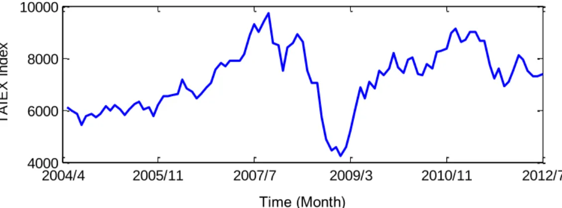
(34) dominant power on the market. Hence, the study attempted to identify the effects of organizational investors on TAIEX Index through the trading value of foreign and other investors. The main approach for studying the fluctuation of stock prices can be categorized as follows: 1. Basic knowledge: analyze the basic situation of the macro-economy and the industries. The macro-economy reflects the integral operation efficacy and establishes the foundation for the further development of the enterprise. Therefore. 政治大 The basic knowledge of the industry includes, financial status, profiting…etc. The 立. both macro-economy and the industries are closely related with the stock prices.. judgment in accordance with only basic knowledge.. 學. ‧ 國. second riches entrepreneur, Warren E. Buffett believes he can make investment. ‧. 2. Technicality: refer to the technical index, trend, and K-charts that reflect the. y. Nat. fluctuation of price. The technical analysis only considers the real pricing. er. io. sit. behaviors in the market or of the financial tools. It is believed that ―the history repeats itself‖ and mass statistic data are used to forecast the direction of trends.. al. n. v i n C h average indictorsUin the technical index to assist The study also adopts the moving engchi trading.. 3. Unexpected situation: when unexpected event occurs, the stock price may have severe fluctuations. From the database of Taiwan Stock Exchange Corporation, only the data of Trading Value of Foreign & Other Investor from April, 2004 to July, 2012 were available therefore the prices of TAIEX Index from April, 2004 to July, 2012 were analyzed. There are five IMFs and one residue exacted from the monthly TAIEX Index data by EEMD. The original data and the results of decomposition are shown in Figure 3.3& 3.4, and the statistical measures are listed in Table 3.4. 34.

(35) TAIEX index. 10000. 8000. 6000. 4000 2004/4. 2005/11. 2007/7 2009/3 Time (Monthly) Time (Month). 2010/11. 2012/7. Figure 3.3 the TAIEX Index from 2004 April to 2012 July. 立. 500 0 -500. Mid IMF4. 2000. y. al. n. 0 -2000. io. HighIMF3. 2000. Nat. -1000. sit. 0. ‧. IMF2. 1000. er. -500. ‧ 國. 0. 學. IMF1. 500. 政治大. Ch. engchi. i n U. v. 2000 0. 0. -2000. -2000. IMF5. Low. 200. 2000 0. 0. -200. Residue Residue. -2000 8000. 8000 7000 7000 6000 6000 2004/4 2005/1 2005/11 2005/11 2006/9 2007/7 2007/7 2008/5 2009/3 2009/3 2004/4 Data Time (Monthly). 2010/12010/11 2010/11 2011/9 2012/7 2012/7. Time (Month). Figure 3.4 the IMF1~ IMF5 and the Residue Decomposed from TAIEX Index 35.

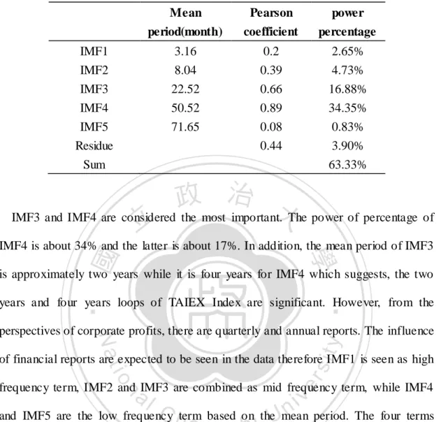
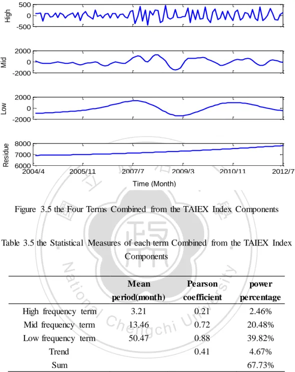
(36) Table 3.4 the Statistical Measures of the Components Decomposed from TAIEX Index Mean. Pearson. power. period(month). coefficient. percentage. IMF1. 3.16. 0.2. 2.65%. IMF2. 8.04. 0.39. 4.73%. IMF3 IMF4. 22.52 50.52. 0.66 0.89. 16.88% 34.35%. IMF5 Residue. 71.65. 0.08 0.44. 0.83% 3.90%. Sum. 63.33%. 政治大 IMF3 and IMF4 are considered the most important. The power of percentage of 立. ‧ 國. 學. IMF4 is about 34% and the latter is about 17%. In addition, the mean period of IMF3 is approximately two years while it is four years for IMF4 which suggests, the two. ‧. years and four years loops of TAIEX Index are significant. However, from the. sit. y. Nat. perspectives of corporate profits, there are quarterly and annual reports. The influence. io. er. of financial reports are expected to be seen in the data therefore IMF1 is seen as high. al. frequency term, IMF2 and IMF3 are combined as mid frequency term, while IMF4. n. v i n C hterm based on theUmean period. The four terms and IMF5 are the low frequency engchi combined from the TAIEX Index components are shown in Figure 3.5.. 36.

(37) High. 500 0 -500. Mid. 2000 0 -2000. Low. 2000 0. Residue. -2000. 8000 7000 6000 2004/4. 2005/11. 立. 政治大 2007/7 2009/3 Time (Monthly). 2010/11. 2012/7. Time (Month). ‧ 國. 學. Figure 3.5 the Four Terms Combined from the TAIEX Index Components. ‧. Table 3.5 the Statistical Measures of each term Combined from the TAIEX Index Components. power percentage. 3.21. 0.21. 2.46%. 0.88. 20.48% 39.82%. 0.41. 4.67%. n. Pearson coefficient. Mid frequency term Low frequency term. Ch. e13.46 ngchi 50.47. Trend Sum. er. io. High frequency term. sit. y. Nat. al. Mean period(month). iv n U 0.72. 67.73%. In Table 3.5, it is shown that the combined IMF has the mean period of approximately three months in the high frequency term, one year in the mid frequency term, and four years in the low frequency term. The influential orders from high to low are low frequency, mid frequency, trend, and high frequency on TAIEX Index. Each frequency and trend is significant and analyzed. 37.

(38) High frequency term It is considered that high frequency term is greatly related to quarterly reports. The organization would also adjust their investments in accordance with quarterly reports. To analyze the correlations between TAIEX Index and organizations, the Trading Value of Foreign & Other Investors was also decomposed as five IMFs and one residue by EEMD. The Trading Value of Foreign & Other Investors of decomposition are shown in Figure 3.6 11. IMF1. 2. x 10. 0 -2. 立. 11. x 10. ‧ 國. 學. IMF2. 1. 政治大. 0 -1. 0. y. sit. 2000 -5. Mid. er. al. n. 0x 1010 -500 5. io. High. -5 500. Nat. IMF3. x 10. 0. IMF4. ‧. 10. 5. 0. Ch. engchi. i n U. v. -2000x 1010. IMF5. 5. Low. 0 2000 -50. -2000 10. Residue Residue. 5. x 10. 8000 0. 7000 -5 6000 2004/4 2004/4. 2005/11 2005/11. 2007/7 2007/7. 2009/3 2009/3 Date Time (Monthly). 2010/11 2010/11. 2012/7 2012/7. Time (Month). Figure 3.6 the IMF1~ IMF5 and the Residue Decomposed from the Trading Value of Foreign & Other Investors 38.

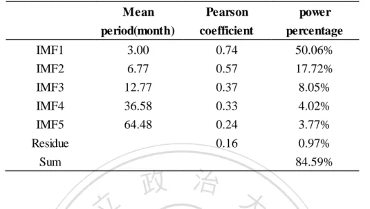
(39) Table 3.6 the Statistical Measures of each term from the Trading Value of Foreign & Other Investors. Mean. Pearson. power. period(month). coefficient. percentage. IMF1 IMF2. 3.00 6.77. 0.74 0.57. 50.06% 17.72%. IMF3. 12.77. 0.37. 8.05%. IMF4 IMF5. 36.58 64.48. 0.33 0.24. 4.02% 3.77%. 0.16. 0.97% 84.59%. Residue Sum. 立. 政治大. From the table 3.6, IMF1 are the most important and the powerful percentage is. ‧ 國. 學. around 50%. The mean period is a three months loop. Pearson correlation between the high frequency term of TAIEX Index and IMF1 were analyzed and shown in Table. ‧. 3.7. The results suggested, there was a 0.75 positive correlation. After comparing with. Nat. sit. y. actual data, such trend is also reflected on the relative high point and low point of. n. al. er. io. high frequency term as well as the IMF1. Figure 3.7 shows the relative high point and. i n U. v. low point. It is concluded, the organization would adjust their position in accordance. Ch. engchi. with the profit of the corporation and the adjustment of position would in turn have effects on the stock market. Nonetheless, there is no significant correlation between high frequency term and original data (0.21) which suggests, the trading behaviors of organizations would not have effects on the price fluctuation of TAIEX Index for the long term.. 39.

(40) High. 500. 0. High. 500 0 -500 -500. 0x 1011 -2000 1. 立. -0.5. 7000 -1.5. 2005/11. 2005/11. 2006/9. Nat. 6000 2004/4 2005/1 2004/4. 2007/7. 2008/5. ‧. 8000 -1. 2009/3. 2010/1. 2007/7 Date 2009/3 Time (Monthly). 2010/11. 2010/11. y. -2000. ‧ 國. Amount IMF1. 0 0. 學. Low. 2000 0.5. Residue. 政治大. 1.5. Time (Month). 2011/9. 2012/7. 2012/7. io. sit. Mid. 2000. n. al. er. Figure 3.7 the Relative High Point and Low Point. Ch. engchi. i n U. v. Table 3.7 The Correlation Coefficients Compared the Trading Value of Foreign & Other Investors to TAIEX Index in terms of High Frequency. Matches of TAIEX Index High Frequency. Pearson. correlation 0.75. 40.

(41) Mid frequency term There is significant correlation between the mid frequency term and original data (0.72). The power percentage is 20% as the second most influential factor for TAIEX Index. The meanings and phenomenon of mid frequency are discussed as follows. The mean period of mid frequency term is around one year, therefore it is considered to be related to the annual reports released by the corporations. The annual reports indicate the annual profits for the corporations. The long-term investors would adjust their position in accordance with the annual reports. In addition, it is shown in many. 政治大. literatures, there are abnormal effects on the stock market and the most noted is January Effect.. 立. ―The January Effect might be the granddaddy of all calendar anomalies, but it is not. ‧ 國. 學. the only one. For inexplicable reasons, stocks generally do much better in the first half. ‧. of the month than the second half, do well before holidays, and plunge in the month of. y. Nat. September. Furthermore, they do exceptionally well between Christmas and New. er. io. sit. Year‘s Day, and until very recently, they have soared on the last trading day of December, which is actually the day that has launched the January Effect. Why these. al. n. v i n well C understood, and whether h e n g c h i U they. anomalies occur is not. will continue to be. significant in the future is an open question. But their discovery has put economists on the spot. No longer can researchers be so certain that the stock market is thoroughly unpredictable and impossible to beat. ‖ (Stocks for the Long Run, 4e, Jeremy J.Siegel) Generally, investors may sell losing stocks to avoid taxes and make another purchase in the next January. Furthermore, the sell-off in December that causes the drop of price also induce buy in and therefore the stock price tends to go up in January. ―If taxes are a factor, however, they cannot be the only one, for the January Effect holds in countries that do not have a capital gains tax. Japan did not tax capital gains for individual investors until 1989, but the January Effect existed before then. 41.

(42) Furthermore, capital gains were not taxed in Canada before 1972, and yet there was a January Effect in that country as well.‖ (Stocks for the Long Run, 4e, Jeremy J.Siegel) In addition, there are other explanation for January Effects. ―There are other potential explanations for the January Effect. Workers often receive extra income, such as from bonuses and other forms of compensation, at year-end.‖ (Stocks for the Long Run, 4e, Jeremy J.Siegel) However, as January Effects attract more attentions, investors now are inclined to use it as the operational strategy so the effects are weakened significantly. Liu (2010) argued that January Effect can be found in the. 政治大 term also show that the prices rose in January, 2005, 2006, 2007, 2009, 2011, and 立. stock market in Taiwan and United Kingdom. The observations on mid frequency. 2012. The reason why there was no January Effect in 2008 and 2010 was due to the. ‧ 國. 學. global financial crisis and European sovereign-debt crisis. Figure 3.8 shows the. y. sit er. al. n. Mid frequency. io. 1000. Nat. 2000. ‧. January Effect.. 0 -1000 -2000. Ch. engchi. i n U. v. 2005/1 2006/1 2007/1 2008/1 2009/1 2010/1 2011/1 2012/1 Time (Monthly) Time (Month). Figure 3.8 the January Effect. The incidents that affect TAIEX Index such as, the Subprime mortgage crisis in 2007, economic crisis in 2008, European sovereign-debt crisis in 2010, enterprise review in 2011, and the utility rise as well as taxation of stock income in 2012, can all be reflected in the mid frequency term. Table 3.8 and Figure 3.9 shows mid-frequency 42.

(43) term can reflect important financial incidents. Table 3.8 Incidents Event. Time. Price. Oct-07. 9859→7384. (2) Global financial crisis. May-08. 9309→3955. (3) European sovereign-debt crisis. Jan-10. 8395→7080. (4) United States debt-ceiling crisis. Aug-11. 8707→6744. 政治 Apr-12 大. 8121→6857. (1) Subprime mortgage crisis. (5) The raise of gas and utilities Implementation of stock income tax. 立. y. sit. European sovereign-debt crisis. al. er. Subprime mortgage crisis. n. Mid frequency. ‧. ‧ 國. 學. io. 1000. Nat. 2000. 0. Ch. engchi. i n U. -1000 Global financial crisis. -2000. The raise of gas and utilities Implementation of stock income tax. v. United States debt-ceiling. 2005/1 2006/1 2007/1 2008/1 2009/1 2010/1 2011/1 2012/1 Time (Monthly) Time (Month). Figure 3.9 the Big Events. 43.

(44) Low frequency term There is significant correlation between the low frequency term and original data (0.88). The power percentage is 40% as the most crucial factor of TAIEX Index. The meanings and phenomenon of low frequency are discussed as follows. The low frequency term is considered related to the booming cycle of TAIEX Index. The booming cycle is also known as economic cycle or business cycle, indicating the circulation trend of recession, depression, recovery, and prosperity of GDP. Business circulation is shown in Figure 3.10 the trend Y indicates Real GDP that is, GDP would increase with trend Y through time even if there is no business circulation.. 政治大. The economics have long-term growth and the growth pace would be determined by. 立. saving rate, population growth, and development of technology. The Real GDP is. ‧ 國. 學. fluctuated when the business circulation occurs.. ‧. n. er. io. sit. y. Nat. al. Ch. engchi. i n U. v. Figure 3.10 Business Cycle. One of the purposes of studies on business circulation is to identify the turning point to prepare for the future economics in advance. Council for Economic Planning 44.

(45) and Development (ECPD) would determine the economic status on the basis of macroeconomics. The leading indicator was chose to make comparisons with low frequency term and according to ECPD, the indicator is consisted with seven factors as follows: Index of export orders、Monetary aggregates, M1B、Stock prices index、 Index of producer's inventory、Average monthly overtime in industry & services、 Building permits (including only housing, mercantile, business and service, industry 7800. warehousing)、SEMI book-to-bill ratio. 7700. The Figure 3.11 and 3.12 shows the comparison of low frequency term and leading 78007600. 政治大 low frequency term is related to booming loop. 立. indicator. The Table 3.9 shows the correlation coefficient is 0.98 which suggests the 77007500. ‧ 國. 0 7100 2000 7300 7800 -1000 7000 1000 7200 7700 -2000 6900 2004/5 2005/4 2006/3 2009/112010/2 2004/5 2005/4 2006/3 0 2005/112007/2 2008/12008/12 2007/7 2009/3 2010/11 2012/7 7100 2004/4 monthly 7600 Time (Monthly) Time (Month) -1000 10 7000 7500Figure 3.11 Low Frequency term from 2004 April to 2012 July -2000 5 2004/5 2005/4 2006/3 2007/2 2008/12008/122009/112010/2 2004/5 2005/4 2006/3 6900 7400 2004/4 2005/11 2007/7 monthly2009/3 2010/11 2012/7 Time (Monthly) 0 10 7300. y. sit. Ch. engchi. i n U. v. Residue. Leading indicator Leading indicator. n. al. er. io. price. ‧. 1000 7200 7400. Nat. Low price frequency. 2000 7300 7500. 學. Residue. 7400 7600. -5 5 7200 -10 0 7100. monthly. -5 7000 -10 6900 2004/4. 2005/11. 2007/7monthly 2009/3 Time (Monthly) Time (Month). 2010/11. Figure 3.12 Leading indicator from 2004 April to 2012 July 45. 2012/7.

(46) Table 3.9 the Correlation Coefficients Compared Leading indicator with TAIEX Index in terms of Low Frequency Matches of TAIEX Index Low Frequency. Pearson correlation 0.98. In addition, the mean period is around four years therefore statistics show the business circulates every four years in the U.S. The reason may be the presidential ―The 政治大 Federal Reserve and U.S. government tend to be more simulative in their monetary 立. election in every four years but how the election impacts stock market?. and fiscal policies building up to the presidential elections to support the present. ‧ 國. 學. administration or party—and then have to deal with the excesses by use of tightening. ‧. and cutbacks into the midterm elections, when there is less at stake. Investors also. sit. y. Nat. tend to get optimistic in the first year of a presidency, with so many promises having. io. er. been made during the election, and then realize that not much will change b y the second year. There may be other influences that we have not yet identified, but this is. al. n. v i n cycle.‖ (The C Great Ahead, Harry S. Dent Jr.) U h eDepression i h ngc. another consistent. Furthermore, some suggest corporations adjust their inventory every four years therefore it may also serve as one of the causes of four year circulation (Kitchin, 1923). Council for Economic Planning and Development in Taiwan points out, the economics in Taiwan has circulated 10 times and the duration for each time as 56 months.. 46.

(47) Trend The long-term trend of index is considered to be influenced by the Real GDP. GDP refers to the market value of all officially recognized final goods and services produced within a country in a given period of time and is generally used to assess the economic performance of a certain country. As shown in Figure 3.10, the economic activities may be fluctuated in short terms yet long term speaking, the accumulation of capital and development of technology would increase GDP. The Figure 3.13 shows the comparison of real GDP and trend and it is observed that they have the same. 政治大. trend.. 立. 7. Nat. 1.1 2004. 2005. 2006. io. 8000. 7500. Trend Price. 2008 year Time (Year). n. al. 2007. y. 1.2. 2009. 2010. 2011. sit. 1.3. er. 1.4. ‧. ‧ 國. 學. Unit: Million NT$. 1.5. x 10. Ch. engchi. i n U. v. 7000. 6500. 2004. 2005. 2006. 2007. 2008 2009 day Time (Month). 2010. 2011. 2012. Figure 3.13 the Comparisons between GDP and Trend from 2004 to 2012 We also compares with GDP and Trend from 1991 to 2011. Long term speaking, the Figure 3.13 shows the comparison of low frequency term and leading indicator 47.

(48) and the Table 3.10 shows the correlation coefficient is 0.98 which suggests, trend and real GDP are closely related no matter whether for long term or short term. According to Table 3.5, the correlation coefficient between trend and real GDP is 0.41 and the power percentage is 4% which indicates trend has less effect on the TAIEX Index number from 2004 to 2012 and the most important is business circulations represented by low frequency term.. 7. 立. 1. 1991. 1999. 2007. 2011. y. sit. n. al. er. io. 7000 6000 5000 4000. 2003 year Time (year). Nat. 8000. Trend Price. 1995. ‧. ‧ 國. 0.5. 政治大. 學. Unit: Million NT$. 1.5. x 10. 1991. 1995. Ch. engchi. 1999. 2003 year Time (year). i n U. v. 2007. 2011. Figure 3.14 Comparisons between GDP and Trend from 1991 to 2011 Table 3.10 the Correlation Coefficients Compared Real GDP with TAIEX index in terms of Trend. Matches of TAIEX Index Trend. Pearson correlation 0.98. 48.

(49) 3.4. Experiment design In the experiment, we input the closing price of 60 days to train to model forecasting the closing price the next day and conduct a successive forecasting of stock price. Three models were used in the study – ARMA model and two different types of EEMD-ANN model. The forecasting accuracies of three models were compared. The forecasting strategy of EEMD-ANN model includes three steps as follows: Step1: extract data. 政治大 Year came across), the business days in other months were 21-23 days with total of 立 Except for there were only 13 business days in February, 2010 (the Chinese New. 250 business days. The closing prices of 60 days previous to the forecasting month. ‧ 國. 學. were used as the beginning input and Moving Window was used to forecast each. ‧. business day in the month. For instance, the closing prices from 2010/6/8 to. sit. y. Nat. 2010/8/31 are the inputs for the forecasting of the closing price of 2010/9/1.. io. er. Step2: EEMD and ANN training. After inputting the TAIEX Futures, the new data – IMFs were generated from the. n. al. Ch. decomposition made by EEMD and IMFs were. engchi. iv n viewed U as. the factor of TAIEX. Futures which were used as input data to construct EEMD-ANN Model 1 and EEMD-ANN Model 2. a. EEMD-ANN Model 1 n+1 sets of IMFs (n sets of IMFs and residue) were produced by decomposing the TAIEX Futures with EEMD, every set of IMF was then input into the corresponding BPN models respectively. Each BPN model was distinguished by their target data. When IMFm (m=1, 2…n+1) are input in BPN m, The IMFm discarded the first point was regarded as the target data. For BPN training, the inputs and target data were put into a BPN network and the discarded last points of IMFs were used as the input for 49.

(50) this trained network to make forecasting. In other words, the IMF of next minute was forecasted and the TAIEX Future could be retrieved by adding each IMF.. 立. 政治大. ‧. ‧ 國. 學. Figure 3.15 Flow Chart of EEMD-ANN Model 1. n. al. er. io. sit. y. Nat b. EEMD-ANN Model 2. i n U. v. Similarly, the procedure in model 2 started with decomposing TAIEX Futures by. Ch. engchi. EEMD, n+1 sets of IMFs were generated while the different part of model 2 from model 1 was that all the IMF m (m=1,2…n+1) were put into BPN at once and data trained were TAIEX Futures without being decomposing. The TAIEX Futures discarded at the starting point was regarded as the target data. In the training of BPN, inputs and target data were put into BPN network and the discarded last point of IMFm (m=1,2…n+1) were used as inputs for the trained network to make forecasting. The point represented the forecasted value of TAIEX Futures.. 50.

(51) 立. 政治大. ‧ 國. 學 ‧. Figure 3.14 Flow chart of EEMD-ANN Model 2. sit. y. Nat. io. er. Step3: Moving window and forecasting. The models used moving window concept to forecast the price of next minute. That. al. n. v i n was, the forecasted value couldC be the reference for trading h e n g c h i U in one minute. While the. actual value of closing price was collected, it could be used to forecast the value of next day and so forth. The three steps repeated every day in 2010.. 51.

(52) 立. 政治大. ‧. ‧ 國. 學. n. er. io. sit. y. Nat. al. Ch. engchi. i n U. v. Figure 3.15 Training Network by Moving Window Process (Model 1). 52.

(53) 立. 政治大. ‧. ‧ 國. 學. n. er. io. sit. y. Nat. al. Ch. engchi. i n U. v. Figure 3.16 Training Network by Moving Window Process (Model 2). 53.

(54) 3.4. Performance Forecasting results The stock price fluctuates in a certain range every day therefore the forecasted value must fall within the range of fluctuation to be accurate. One of the most common charts in the market is called candlestick chart or K-chart which composed with opening price, closing price, highest price, and lowest price. Generally, the red line represents the rise of stock price (closing price higher than opening price) and green line represents the fall of stock price (closing price lower than opening price).. 政治大 prices extended above and below from real body are called shadows. The trade is 立. Zone between opening and closing is call real body while the highest and lowest. good and the forecast is accurate when the forecasted price falls between the highest. ‧ 國. 學. and lowest prices of the minute which is very important because the forecasted value. ‧. can only be used to establish the trading strategies when the trading is good. An. y. sit. io. n. al. er. 7950. Nat. example of K-chart is demonstrated as Figure 3.19:. Price. 7900. Ch. Shadow. engchi. i n U. v High Close. 7850 Real Body. Open 7800 Low 7750. 7700 2010/3/26 Time (Day). Figure 3.19 the Shape of a Candlestick 54. Time(Day).

(55) For example, the data of opening, closing, highest, and lowest prices are as follows:. Table 3.11 the Example of TAIEX Futures Time. Open. High. Low. Close. 2010/12/27 2010/12/28. 8867 8919. 8908 8919. 8829 8840. 8892 8871. When the closing price at 2010/12/7 is 8892, the TAIEX Future forecasted in next day will fall between 8919 and 8840 for the forecast to be accurate and the stock can. 政治大. be traded successfully as shown in the Figure 3.20:. 立. y. sit. Price. 8800. 8863. al. 8840. n. 8820. io. 8840. Nat. 8860. ‧. 8880. Close. er. 8900. 8919. 學. 8920. ‧ 國. 8940. Ch. engchi. i n U. v. 8780 2010/12/27. 2010/12/28. Time(Day). Time (Day). Figure 3.20 Trade Success. On the other hand, when the forecasted price falls outside of the range between highest and lowest prices – assuming the forecasted price is 8803 – it means the forecast is inaccurate and the trade is unable to be proceeded.. 55.

(56) 8940 8919. 8920 Close 8900. Price. 8880 8860 8840 8840. 8820 8803. 8800 8780 2010/12/27. 立. 政治大. 2010/12/28. Time(Day). Time (Day). Figure 3.21 Trade Failure. ‧ 國. 學 ‧. By using the methods mentioned above, the accuracies of two models were. io. al. y. ccu te fo ec sts tot l fo ec sts. sit. (%) =. 00%. er. Nat. examined by the formula shown below:. v. n. Generally, there are two quotations in the stock market – quotation fluctuation and. Ch. engchi. i n U. quotation trend. The business days in 2010 were divided into two parts – first half from January to June and latter half from July to December. The Figure 3.22 & 3.23 shows the market fluctuated more acutely in the first half year of 2010 (quotation fluctuation) while the fluctuation from July to December were milder (quotation trend). The forecasting accuracies of three models in these two quotations were compared.. 56.