二維平滑熱帶環面法諾曲體之研究 - 政大學術集成

全文

(1)� � � � � � � � � � � ��. On Two-Dimensional Smooth Tropical Toric Fano Varieties. ��. �� : �� : �� .

(2) �� , ��: �� , ��, � ��, �� , �� , �� , �� , ��, �� , ��, ��, �� , ��, ��, �� , ��, ��, �� , ��, ��, � ��, �� , ��, ��, �� , ��, ��, � ��, �� , �� , ��, �� , �� , ��, �� i.

(3) ��, �� , �� , ��, �� , ��, ��, �� , ��, �� , �� , �� , ��, �� , ��, ��, �� , �� , ��, �� , ��, �� , �� , ��, �� , ��, ��, �� , ��, �� , ��, ��, �� , �� , �� , ��, ��, �� , ��, �� ,. ii.

(4) ��, ��, �� (��), �� , ��, �� , ��, �� , ��, �� , ��. iii.

(5) Abstract. In this thesis, we survey and study tropical toric varieties with focus on tropical toric Fano varieties. To construct tropical toric varieties, we start with fans, just like the situation in classical algebraic geometry. However, some constructions does not make sense in tropical settings. Therefore, we need to choose a reasonable definition which give an analogue of a classical toric variety. In the end of this paper, we use the definition we choose, and explicitly calculate all smooth two-dimensional tropical toric Fano varieties which we found are very similar to classical cases.. iv.

(6) �� , ��, �� , ��, �� , ��, �� , ��, �� , ��. v.

(7) Contents ��. i. Abstract. iv. ��. v. 1 Introduction. 1. 2 Background. 4. 2.1. Non-Archimedean amoebas . . . . . . . . . . . . . . . . . . . .. 4. 2.2. Semifield . . . . . . . . . . . . . . . . . . . . . . . . . . . . . .. 9. 2.3. Tropical Semifields . . . . . . . . . . . . . . . . . . . . . . . . 12. 3 Toric variety and Fano variety. 17. 3.1. Polyhedral Geometry . . . . . . . . . . . . . . . . . . . . . . . 17. 3.2. Fiber products of affine varieties . . . . . . . . . . . . . . . . . 33. 3.3. Toric Varieties . . . . . . . . . . . . . . . . . . . . . . . . . . . 38. 3.4. Fano varieties . . . . . . . . . . . . . . . . . . . . . . . . . . . 48. 4 Tropical Toric Variety 4.1. 50. K(G, R, M ) . . . . . . . . . . . . . . . . . . . . . . . . . . . . 50. vi.

(8) 4.2. Tropical Toric Variety . . . . . . . . . . . . . . . . . . . . . . 67. 4.3. Smooth two-dimensional tropical toric Fano varieties . . . . . 72. Bibliography. 95. vii.

(9) Chapter 1. Introduction. The tropical geometry is a relatively recent subject in the field of mathematics. Why does it have an adjective ”tropical”? In the 1980s, Imre Simon (August 14, 1943 - August 13, 2009) who is a Hungarian-born Brazilian mathematician and computer scientist pioneered the tropical geometry. The word ”tropical” was coined by some French mathematicians in honor of Imre Simon, because they thought Brazil is a tropical country. Hence there is not any deeper meaning in an adjective ”tropical”, and this is why the tropical geometry is not called ”temperate geometry” or ”frigid geometry”. Why the mathematicians attend to the tropical geometry in recent years? Because Grigory Mikhalkin has proven that the number of simple tropical. 1.

(10) curves (counted with appropriate multiplicities) of degree d and genus g that pass through g + 3d − 1 generic points in R2 is equal to the Gromov-Witten number Ng,d of the complex projective plane CP2 , so the theorem is called Mikhalkin’s correspondence theorem, see [19]. The main reference is the paper [17] by Henning Meyer. Some difference are that we prove some propositions and provide more details with examples and figures. Moreover, this paper main discusses about the smooth tropical toric Fano varieties on two dimensional. The tropical toric variety and toric varieties have the similar properties, for example, the tropical toric variety X∆ (T) � TP2 where TP is the tropical projective space in the Example 4.3.2, and the toric variety X∆ (T) � CP2 where CP is the complex projective space in the Example 3.3.18. The structure of the paper is as follows. In chapter 2, we recall the semigroup, semiring and semifield, and introduce amoebas and the tropical geometry where the tropical semifield (T, ⊕, ⊙) is a semifield with two operations a ⊕ b := max{a, b} and a ⊙ b := a + b. Note that some papers or books may be defined the tropical sum by a ⊕ b := min{a, b} (e.g. [15]), in fact, the algebraic structures of max-algebra and min-algebra are isomorphic. For more information see [13], [20], [10], [23] and [26].. 2.

(11) In chapter 3, we review some basic concepts of polyhedral geometry and explain how they relate to toric varieties. For more details see [5], [22], [14], [12], [11], [4], [28], [24] and [16]. And we will give a brief introduction to Fano varieties and Fano polytopes. For careful statement see [14], [22] and [5]. In the first part of the chapter 4, we describe the relationship between K(G, R, M ), hom(S, M ), and explain the relationship between the algebraic structures of K(G, R, M ) and the algebraic structures of M . In the setion 2 and 3 of chapter 4, we explain the properties of tropical toric varieties, and calculate five types of the smooth tropical toric Fano varieties.. 3.

(12) Chapter 2. Background. The chapter contains some basic definitions and propositions from tropical geometry.. 2.1. Non-Archimedean amoebas. In this section, we recall the valuation and amoebas. And we set C∗ = C \ {0} in this paper. Let K be an algebraic closed field (e.g. C), and let An denote an affine n-space over K.. 4.

(13) Firstly, we define a map Log : (C∗ )n → Rn by. Log(z1 , . . . , zn ) = (log |z1 |, . . . , log |zn |).. Let u = (u1 , . . . , un ) be in Zn , then we said that z u := z1u1 z2u2 · · · znun is the Laurent monomial. Moreover, the Laurent polynomial f is a finite linear combination of Laurent monomials, that is, f =. �. u∈Zn. au z u where au is in. a field F (as C) and is only finitely many. Denoted by F [z1±1 , . . . , zn±1 ] is the ring of Laurent polynomials in n variables over F . Definition 2.1.1. An affine algebraic variety is the common zero set of a collection {Fi }i∈I of complex polynomials. We write. V = V({Fi }i∈I ) = {(x1 , . . . , xn ) ∈ Cn | Fi (x1 , . . . , xn ) = 0 ∀ i ∈ I}. where Fi = Fi (x1 , . . . , xn ) ∈ Cn [x1 , . . . , xn ] Example 2.1.2. There are some trivial cases of algebraic varieties.. (1) V(0) = An . (2) V(1) = ∅. (3) V(x1 − a1 , . . . , xn − an ) = {(a1 , . . . , an )}. 5.

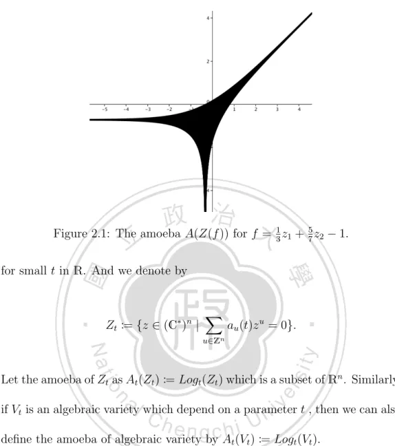
(14) For any subset S of C∗ [z1±1 , . . . , zn±1 ], we denote by. Z(S) := {z ∈ (C∗ )n | f (z) = 0 for all f ∈ S},. that is, Z(S) is the common zero set of a collection {fi }i∈I of Laurent polynomials in a subset S of C∗ [z1±1 , . . . , zn±1 ]. Definition 2.1.3. We define the amoeba of Z(S) as A(Z(S)) := Log(Z(S)) which is a subset of Rn . Remark 2.1.4. Let V be an algebraic variety, then we can also define the amoeba of algebraic variety by A(V ) := Log(V ). Example 2.1.5. Let f =. 1 z 3 1. + 57 z2 − 1 in C∗ [z1 , z2 ]. If f = 0, then. 7 7 z2 = − 15 z1 + 75 , and so V(f ) = {(t, − 15 t + 75 )|t ∈ C}. Then A(V(f )) =. Log(V(f )) = (log |t|, log | −. 7 t 15. + 75 |).. For more information about the amoebas see [11] chapter 6 and [27]. The figure of the amoeba is used for GeoGebra (Curve[ln(abs(t)), ln(abs(exp(−5/7)− t ∗ exp(−8/21))), t, −100, 100]) or we can also use for maple, for more details see [1]. Next, we define a map Logt : (C∗ )n → Rn by. Logt (z1 , . . . , zn ) = (logt |z1 |, . . . , logt |zn |) 6.

(15) Figure 2.1: The amoeba A(Z(f )) for f = 13 z1 + 57 z2 − 1. for small t in R. And we denote by. Zt := {z ∈ (C∗ )n |. �. au (t)z u = 0}.. u∈Zn. Let the amoeba of Zt as At (Zt ) := Logt (Zt ) which is a subset of Rn . Similarly, if Vt is an algebraic variety which depend on a parameter t , then we can also define the amoeba of algebraic variety by At (Vt ) := Logt (Vt ). We recall that the Hausdorff distance. Let (M, d) be a metric space, and let A and B be two non-empty subsets of (M, d). Then we define the Hausdorff distance dH (A, B) between A and B by. dH (A, B) = max{sup inf d(a, b), sup inf d(a, b)}. a∈A b∈B. 7. b∈B a∈A.

(16) On Rn , the subsets At converges to A as t → ∞ in the Hausdorff metric on compacts, that is, for any compact set D in Rn , and there exists a neighborhood U of D such that dH (At ∩ U, A ∩ U ) → 0 as t → ∞ ([13], Prop. 1.2 and [18], Prop. 1.6 ). Definition 2.1.6. The set C{{t}} is called the field of Puiseux series with complex coefficients if C{{t}} is the set of all formal power series a(t) = �. q∈Q. aq tq where aq is in C∗ and {q} is bounded below and has a finite set of. denominators, that is, ∞ � C{{t}} := { ai ti/n | ai ∈ C∗ , m ∈ Z, n ∈ Z≥0 }. i=m. We set C{{t}} = K from now on. Definition 2.1.7. Let K be a field of Puiseux series. A non-Archimedean valuation on K is a function. val : K → R ∪ {−∞}. satisfying the properties:. (i) val(a) = −∞ if and only if a = 0, (ii) val(ab) = val(a) + val(b), 8.

(17) (iii) val(a + b) ≤ max{val(a), val(b)}. For each a in K with a �= 0, we define the valuation of a by val(a) = min{q | aq �= 0} (since {q} is bounded below). And we define a norm by |a|val := exp(val(a)). Let VK be an algebraic variety on (K ∗ )n , we define a map V al : (K ∗ )n → Rn by. V al(z1 , . . . , zn ) = (log |z1 |val , . . . , log |zn |val ) = (val(z1 ), . . . , val(zn )).. Then we can also define the amoeba of algebraic variety VK on (K ∗ )n by A(VK ) := V al(Vt ). Theorem 2.1.8 (a version of Viro patchworking). Let Vt be an algebraic variety for small t in R, and let VK be an algebraic variety on (K ∗ )n , then the non-Archimedean amoeba A(VK ) is the limit of the amoebas At (Vt ) as t → ∞ with respect to the Hausdorff metric on compacts.. 2.2. Semifield. In this section, we will introduce the semigroup, semiring, and semifield. Definition 2.2.1. Let G be a nonempty set. A binary operation in G is a function ∗ : G × G → G. We denote the element f (a, b) of G by a ∗ b for all 9.

(18) (a, b) ∈ G. The set G is said to be closed under the binary operation ∗ and denoted by (G, ∗). The usual addition and multiplicative are two binary operations on R. Definition 2.2.2. A semigroup is a nonempty set G together with a binary operation ∗ which satisfies associative, that is, (a ∗ b) ∗ c = a ∗ (b ∗ c) for all a, b, c ∈ G. A semigroup (G, ∗) is called a commutative if a ∗ b = b ∗ a for all a, b ∈ G. A semigroup (G, ∗) is called idempotent if a ∗ b ∈ {a, b} for all a, b ∈ G. Definition 2.2.3. A monoid is a semigroup G with an identity element e, that is, a ∗ e = e ∗ a = a for all a ∈ G. Proposition 2.2.4. Every group is a monoid.. Proof. Let G be a group. According to the definition of group, G is closed under a binary operation ∗, and G satisfies associative and has an identity element e, hence G is a monoid. Example 2.2.5. Let (2Z>0 , ∗) be the set of the positive even integers under the usual multiplication of real numbers. Suppose that x, y, and z belong to 2Z>0 , then x ∗ (y ∗ z) = (x ∗ y) ∗ z, so 2Z>0 satisfies associative. But 1 is not 10.

(19) even, that is, 1 is not in 2Z>0 , so 2Z>0 does not have an identity element. Hence (2Z>0 , ∗) is a semigroup which is not a monoid. Definition 2.2.6. Let S1 and S2 be semigroup. A map ψ : S1 → S2 is a morphism of semigroup if ψ(xy) = ψ(x)ψ(y) for all x, y in S1 . Example 2.2.7. Define a map φ : (Z>0 , +) → (Z4 , +) by φ(x) = x¯, for all x in Z>0 . For all x, y in Z>0 , φ(x + y) = x + y = x¯ + y¯ = φ(x) + φ(y). Hence φ is a morphism of semigroup. Definition 2.2.8. A semiring is a nonempty R together with two binary operations ⊕ : R × R → R and ⊗ : R × R → R such that (R, ⊕) is a commutative monoid with identity element 0R , (R, ⊗) is a semigroup, and the operation ⊗ distributes over ⊕, that is, a ⊗ (b ⊕ c) = a ⊗ b ⊕ a ⊗ c where a, b, c are in R. Note that, according to the definition of ring, every ring is a semiring. Definition 2.2.9. A semifield is a semiring (R, ⊕, ⊗) together with (R\{0R }, ⊗) is an abelian group where 0R is an identity element for the binary operation ⊕. Note that, by the definition of ring, every field is a semifield. 11.

(20) Example 2.2.10. Let T = R ∪ {−∞}. We define two operations on T by a ⊕ b := max{a, b} and a ⊙ b := a + b. Suppose that a and b, and c are in T. Without loss of generality, assume that a ≥ b. Becuase a ⊕ b = max{a, b} = a is in T, so T is closed under a binary operation ⊕. If a and b are in R, then a ⊙ b = a + b is in R; if one of a and b is −∞, then a ⊙ b = −∞, and so T is closed under a binary operation ⊙. Suppose that a, b, and c are in T. Without loss of generality, assume that a ≥ b ≥ c. Because a ⊕ (b ⊕ c) = max{a, max{b, c}} = max{a, b} = a and (a ⊕ b) ⊕ c = max{max{a, b}, c} = max{a, c} = a, so a ⊕ (b ⊕ c) = (a ⊕ b) ⊕ c, i.e. (T, ⊕) is a semigroup. Since −∞ ⊕ a = a ⊕ −∞ = a, −∞ is an identity element, and so a⊕b = b⊕a = max{a, b}, that is, (T, ⊕) is a monoid with identity element −∞. Moreover, a⊕b = max{a, b} = b⊕a, so (T, ⊕) is a commutative monoid. Since (T\{−∞}, ⊙) = (R, +) is abelian group, (T, ⊕, ⊙) is a semifield. The above T will be discussed in more details in the next section.. 2.3. Tropical Semifields. Definition 2.3.1. Let T = R ∪ {−∞}. The tropical semifield (T, ⊕, ⊙) is the semifield with operations a ⊕ b := max{a, b} and a ⊙ b := a + b. (c.f. Example 2.2.10) 12.

(21) Remark 2.3.2. Since (T\{−∞}, ⊙) is an abelian group, we can define the tropical division by x � y := x − y, for all x and y in T\{−∞}. Proposition 2.3.3. (a) Both addition and multiplication are commutative: x ⊕ y = y ⊕ x and x ⊙ y = y ⊙ x. (b) The distributive law holds for tropical addition and tropical multiplication: x ⊙ (y ⊕ z) = x ⊙ y ⊕ x ⊙ z. Proof. (a). (i) x ⊕ y = max{x, y} = max{y, x} = y ⊕ x.. (ii) x ⊙ y = x + y = y + x = y ⊙ x. (b) x ⊙ (y ⊕ z) = x + (y ⊕ z) = x + max{y, z} = max{x + y, x + z} = (x + y) ⊕ (x + z) = x ⊙ y ⊕ x ⊙ z. Remark 2.3.4. For all integer n and all x in T, we define. x⊙n := x ⊙ · · · ⊙ x =. n �. x = nx.. i=1. Note that −∞ is the additive identity and zero is the multiplicative unit, that is, x ⊕ (−∞) = x and x ⊙ 0 = x. Definition 2.3.5. The Rn is a module over the tropical semiring 13.

(22) (R ∪ {∞}, ⊕, ⊙), with the operations of coordinatewise tropical addition. (a1 , · · · , an ) ⊕ (b1 , · · · , bn ) = (max{a1 , b1 }, · · · , max{an , bn }). and tropical scalar multiplication. λ ⊙ (a1 , · · · , an ) = (λ + a1 , · · · , λ + an ). Definition 2.3.6. Let (M, ⊕M ) be a commutative monoid over tropical semifield T. Then M is called a tropical module if there exists a scalar multiplication ⊙M : T × M → M denoted by ⊙M (t, m) = t ⊙M x for all t in T and x in M , such that for all t1 , t2 in T and x, y in M ,. (i) t1 ⊙M (x ⊕M y) = (t1 ⊙M x) ⊕M (t1 ⊙M y); (ii) t1 ⊙M (t2 ⊙M x) = (t1 ⊙ t2 ) ⊙M x; (iii) 1T ⊙M x = x where 1T = 0 is the multiplicative identity of T; (iv) if t1 ⊙M x = t2 ⊙M x then either t1 = t2 or x = −∞. For careful statements, we refer the reader to [21]. Definition 2.3.7. A T-vector space or tropical vector space M over T consists of a commutative monoid (M, ⊕M ) and ⊙M : T × M → M such that 14.

(23) for all t1 , t2 in T, x, y in M , we have:. (i) t1 ⊙M (x ⊕M y) = (t1 ⊙M x) ⊕M (t1 ⊙M y); (ii) t1 ⊙M (t2 ⊙M x) = (t1 ⊙ t2 ) ⊙M x; (iii) 1T ⊙M x = x for the tropical multiplicative identity 1T . (iv) (t1 ⊕ t2 ) ⊙M x = (t1 ⊙M x) ⊕M (t2 ⊙M x); Definition 2.3.8. The tropical projective n-space, denoted by TPn , is defined as the quotient. (Tn+1 \ (−∞, . . . , −∞)). �. ∼,. where ∼ denotes the equivalence relation, (x0 , . . . , xn ) ∼ (y0 , . . . , yn ) if and only if there exists a λ in T∗ such that (y0 , . . . , yn ) = (λ ⊙ x0 , . . . , λ ⊙ xn ) = (λ + x0 , . . . , λ + xn ). Definition 2.3.9. Fix a weight vector ω = (ω1 , . . . , ωn ) ∈ Rn . The weight of the variable xi is ωi . The weight of a term p(t) · xα1 1 · · · xαnn is the real number. order(p(t)) + α1 ω1 + · · · + αn ωn .. Definition 2.3.10. The tropical monomial is defined to be an expression of 15.

(24) the form c ⊙ xa11 ⊙ · · · ⊙ xann where a1 , · · · , an ∈ Z≥0 and c is a constant. Definition 2.3.11. The finite linear combination of tropical monomials is called a tropical polynomial. Namely, f = c1 ⊙ xa111 ⊙ · · · ⊙ xan1n ⊕ · · · ⊕ ck ⊙ xa1k1 ⊙ · · · ⊙ xankn Definition 2.3.12. Consider a polynomial f ∈ C[x1 , . . . , xn ] and a vector ω ∈ Rn , the initial form inω (f ) is the sum of all terms in f of smallest ω-weight. Definition 2.3.13. The tropical hypersurface of f is the set. T (f ) = {ω ∈ Rn | inω (f ) is not a monomial}.. Remark 2.3.14. All of points ω of the T (f ) are attained by at least two of the linear functions. Note that T (f ) is invariant under dilation, so we can say T (f ) by giving its intersection with the unit sphere. (See [2] and the references therein). 16.

(25) Chapter 3. Toric variety and Fano variety. We begin by recalling the some basic definitions and notations which are necessary for study tropical toric varieties.. 3.1. Polyhedral Geometry. In this section, we will recall the polyhedral geometry since they relate to affine toric varieties and tropical toric varieties. Definition 3.1.1. Let R be a ring. A right R-module M over R is an abelian group, usually written additively, and an operation M × R → M (denoted (m, r) �→ mr) such that for all r, s in R, x, y in M , we have: 17.

(26) (i) (x + y)r = xr + yr. (ii) x(r + s) = xr + xs. (iii) (xs)r = x(sr). (iv) x1R = x if R has multiplicative identity 1R .. Similarly, we can define a left R-module via an operation R × M → M denoted (m, r) �→ rm and satisfy the above conditions. If R is a ring with identity, then a right R-module is also called a unitary right R-module. If R is a commutative ring, then a right R-modules are the same as left R-modules with mr = rm for all m in M , r in R and are called R-modules. If R is a field, then a R-module M is called a vector space. Definition 3.1.2. An abelian group F is called a free abelian group if it has a basis. Example 3.1.3. The trivial group {0} is the free abelian group on the empty basis. Definition 3.1.4. Let R be a ring. Let M be a right module and N be a left module over R. Let F be the free abelian group on M × N . Let K be the subgroup of F generated by all elements of the forms (i) (a + b, c) − (a, c) − (b, c); (ii) (a, c + d) − (a, c) − (a, d);. 18.

(27) (iii) (ar, c) − (a, rc), for all a, b ∈ M ; c, d ∈ N ; r ∈ R. The quotient group F/K is called the tensor product of M and N , and we write M ⊗R N or simply M ⊗N forF/K. The element (a, c) in F/K is denoted by a ⊗ c. We denote by N � Zn the free abelian group and NR := N ⊗Z R the associated real vector space; moreover, we denote by M := hom(N, Z) the dual lattice of N and MR := M ⊗Z R. Definition 3.1.5. The polyhedron P is the intersection of finitely many halfspaces in NR , that is, a set of the form. P = {X ∈ NR | AX ≥ b}. where A ∈ (NR∨ )d and b ∈ Rd . If A ∈ (N ∨ )d , b ∈ Zd , then P is called a rational polyhedron. If A ∈ (N ∨ )d , b ∈ Rd , then P is called polyhedron with rational slopes. Example 3.1.6. Let A =. �. 1 2 3 4. �. � � 1 and b = , then 2. P = {X ∈ R2 | AX ≥ b} = {(x, y) ∈ R2 | x + 2y ≥ 1, 3x + 4y ≥ 2}. 19.

(28) Figure 3.1: rational polyhedron Definition 3.1.7. For every finite set S ⊆ Rd , if a set S is not convex set, the convex hull of S is the smallest convex set containing it, which we denote it by conv(S), that is,. conv(S) :=. �. {K ⊆ Rd | S ⊆ K, K is a convex set}. . Proposition 3.1.8. Let S be a finite subset of Rn . Then. conv(S) = {λ1 x1 + · · · + λm xm | x1 , . . . , xm ∈ S, λi ≥ 0,. m �. λi = 1}. i=1. � Proof. For any finite set {x1 , . . . , xm } ⊆ S, λi ≥ 0 with m i=1 λi = 1. �� m λ i xi We have λ1 x1 + · · · + λm xm = (1 − λm ) + λm xm for λm < i=1 1−λm 20.

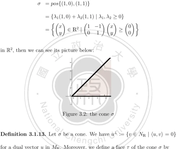
(29) �m. 1. Therefore,. i=1. λi xi ∈ conv(S). Conversely, for any finite set S0 =. {x1 , . . . , xm } ⊆ S, conv(S0 ) = {λ1 x1 + · · · + λm xm | x1 , . . . , xm ∈ S0 , λi ≥ 0,. �m. i=1. λi = 1} ⊆ conv(S). So conv(S) = {λ1 x1 +· · ·+λm xm | {x1 , . . . , xm } ⊆. S, λi ≥ 0,. �m. i=1. λi = 1}. Hence if S = {x1 , . . . , xm } ⊆ Rn is a finite set, then. we have conv(S) = {λ1 x1 +· · ·+λm xm | x1 , . . . , xm ∈ S, λi ≥ 0,. �m. i=1. λi = 1}.. Definition 3.1.9. For every finite set S in a real vector space, the positive hull or conical hull of S is denoted by pos(S) and is the set. pos(S) = {. � i∈I. λi mi | {mi }i∈I ⊆ S, λi ≥ 0}.. Note that if S = ∅, then pos(∅) = {0}. Definition 3.1.10. The Minkowski sum of two sets X and Y in a vector space, defined by X + Y , is the set {x + y | x ∈ X, y ∈ Y } Definition 3.1.11. A set σ is called a polyhedral cone (or simply a cone later) if � σ = pos(S) = { λi mi | {mi }i∈I ⊆ S, λi ≥ 0} i∈I. where S ⊆ NR is finite. By the Minkowski-Weyl theorem for cones, the cone σ is a finitely generated if and only if σ = {X ∈ NR | AX ≥ 0} where A ∈ (MR )d and b ∈ Rd . 21.

(30) (i.e. σ is a polyhedron). For more details see [28] Section 1.3, [4] Theorem 1.15, and [16] p. 88. Example 3.1.12. Consider the cone σ = pos{(1, 0), (1, 1)} = {λ1 (1, 0) + λ2 (1, 1) | λ1 , λ2 ≥ 0} �� x 1 −1 x 0 2 = ∈R | ≥ y 0 1 y 0 in R2 , then we can see its picture below:. Figure 3.2: the cone σ. Definition 3.1.13. Let σ be a cone. We have u⊥ := {v ∈ NR | �u, v� = 0} for a dual vector u in MR . Moreover, we define a face τ of the cone σ by. τ := σ ∩ u⊥ = {v ∈ σ | �u, v� = 0}.. Definition 3.1.14. Let τ and σ be nonempty polyhedra. τ is called a f acet of σ if τ is a face of σ and dim(τ ) + 1 = dim(σ) (denoted by τ ≺ σ), that is, a facet τ is a face of codimension 1. 22.

(31) Definition 3.1.15. A polyhedral cone σ is said a pointed cone if the origin is a face of σ. Otherwise, the polyhedral cone is called a blunt. Example 3.1.16. In R, C1 = {x ∈ R | x ≥ 0} is a pointed cone, and C2 = {x ∈ R | x > 0} is a blunt. Definition 3.1.17. A cone σ is called simplicial if it is generated by a linearly independent subset of the lattice N , that is, σ = pos(C) is called simplicial cone if C is linearly independent. Definition 3.1.18. A simplicial cone σ is called unimodular if it is generated by a subset of a basis of the lattice N . Example 3.1.19. Let N = Z(1, 0) ⊕ Z(0, 1). We consider the cone σ = pos{(1, 0), (3, 2)} in N . Then {(1, 0), (3, 2)} is linearly independent, but (2, 1) is not in Z≥0 (1, 0) ⊕ Z≥0 (3, 2)}. Hence the cone σ is simplicial. Example 3.1.20. Let N = Z(1, 0)⊕Z(0, 1). Given the cone σ = pos{(1, 0), (1, 1)} in N . Then {(1, 0), (1, 1)} is a linearly independent set, and Z≥0 (1, 0) ⊕ Z≥0 (1, 1)} can generate all of integer vectors in the cone σ. Hence the cone σ is unimodular. Definition 3.1.21. The set P = conv(S) = { 0,. �. i∈I. �. i∈I. λi mi | {mi }i∈I ⊆ S, λi ≥. λi = 1} is said a polytope in NR where S ⊆ NR is finite.. 23.

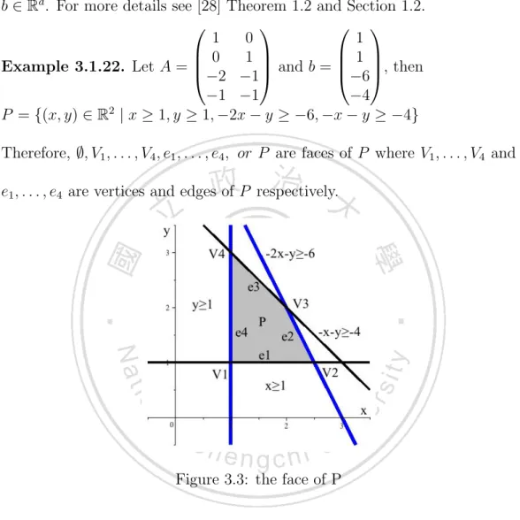
(32) The P = conv(S) + pos(V ) for some finite sets S, V in NR if and only if P is a polyhedron, that is, P = {X ∈ NR | AX ≥ b} where A ∈ (MR )d and b ∈ Rd . For more details see [28] Theorem 1.2 and Section 1.2.     1 0 1 0    1  1 , then Example 3.1.22. Let A =  and b = −2 −1 −6 −1 −1 −4 2 P = {(x, y) ∈ R | x ≥ 1, y ≥ 1, −2x − y ≥ −6, −x − y ≥ −4} Therefore, ∅, V1 , . . . , V4 , e1 , . . . , e4 , or P are faces of P where V1 , . . . , V4 and e1 , . . . , e4 are vertices and edges of P respectively.. Figure 3.3: the face of P Definition 3.1.23. Let f ∈ C[x1 , . . . , xn ], and write f =. �. α∈Zn ≥0. cα xα . The. Newton polytope of f , denoted N P (f ) or N ew(f ), is the lattice polytope. N ew(f ) = conv({α ∈ Z≥0 | cα �= 0}).. 24.

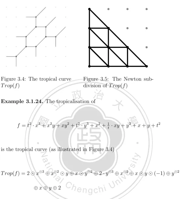
(33) Figure 3.4: The tropical curve T rop(f ). Figure 3.5: The Newton subdivision of T rop(f ). Example 3.1.24. The tropicalisation of. f = t2 · x3 + x2 y + xy 2 + t2 · y 3 + x2 + 1t · xy + y 2 + x + y + t2. is the tropical curve (as illustrated in Figure 3.4). T rop(f ) = 2 ⊙ x⊙3 ⊕ x⊙2 ⊙ y ⊕ x ⊙ y ⊙2 ⊕ 2 · y ⊙3 ⊕ x⊙2 ⊕ x ⊙ y ⊙ (−1) ⊕ y ⊙2 ⊕x⊕y⊕2 = max{2 + 3x, 2x + y, x + 2y, 2 + 3y, 2x, x + y − 1, 2y, x, y, 2}. The vertices of the tropical curve are:. (2, 0), (1, 1), (1, 0), (0, 2), (0, 1), (0, −1), (−1, 0), (−1, −1), (−2, −2). 25.

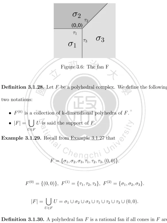
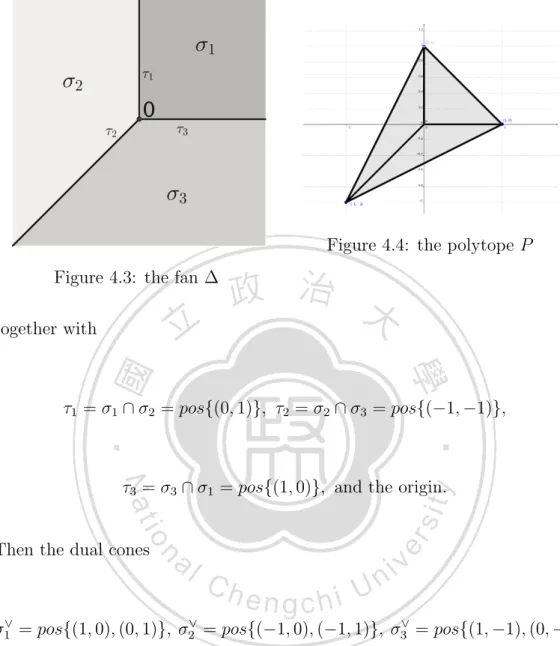
(34) The Newton subdivision of the tropical curve T rop(f ) is. N ew(T rop(f )) = conv{(0, 0), (1, 0), (2, 0), (3, 0), (0, 1), (0, 2), (0, 3), (1, 1), (1, 2), (2, 1)}.. We illustrate the Newton subdivision of in Figure 3.5. Definition 3.1.25. A polyhedral complex ∆ is a collection of polyhedra such that the following the two conditions are satisfied: if U ∈ ∆ and F is a face of U , then F ∈ ∆; if U, V ∈ ∆, then U ∩ V is a face of U and V . The empty set is in the polyhedral complex ∆, i.e. a polyhedral complex ∆ contains empty face. Definition 3.1.26. F is a polyhedral fan if F is a polyhedral complex and each σ in F is a cone.. Note that we consider the fan is collection of non-empty polyhedral cones in this paper. Example 3.1.27. Suppose that τ1 = pos{(−1, 0)}, τ2 = pos{(1, 1)}, τ3 = pos{(0, −1)}, σ1 = pos{(−1, 0), (0, −1)}, σ2 = pos{(−1, 0), (1, 1)}, and σ3 = pos{(0, −1), (1, 1)} Let F = {(0, 0), τ1 , τ2 , τ3 , σ1 , σ2 , σ3 }}. Then (0, 0) is the face of other elements of F and (0, 0) = τ1 ∩ τ2 = τ1 ∩ τ3 = τ2 ∩ τ3 , τ1 = σ1 ∩ σ2 26.

(35) is the face of σ1 and σ2 , τ2 = σ2 ∩ σ3 is the face of σ2 and σ3 , τ3 = σ1 ∩ σ3 is the face of σ1 and σ3 . Hence F is a fan.. Figure 3.6: The fan F. Definition 3.1.28. Let F be a polyhedral complex. We define the following two notations: • F (k) is a collection of k-dimendional polyhedra of F . � • |F | = U is said the support of F . U ∈F. Example 3.1.29. Recall from Example 3.1.27 that. F = {σ1 , σ2 , σ3 , τ1 , τ2 , τ3 , (0, 0)}.. F (0) = {(0, 0)}, F (1) = {τ1 , τ2 , τ3 }, F (2) = {σ1 , σ2 , σ3 }. |F | =. �. U ∈F. U = σ1 ∪ σ2 ∪ σ3 ∪ τ1 ∪ τ2 ∪ τ3 ∪ (0, 0).. Definition 3.1.30. A polyhedral fan F is a rational fan if all cones in F are rational polyhedra. 27.

(36) Definition 3.1.31. A polyhedral fan F in a vector space NR is complete if the support of F is NR , i.e. |F | = NR . Example 3.1.32. Recall from Example 3.1.27 that F = {σ1 , σ2 , σ3 , τ1 , τ2 , τ3 , (0, 0)}. � Then |F | = U = σ1 ∪ σ2 ∪ σ3 ∪ τ1 ∪ τ2 ∪ τ3 ∪ (0, 0) = R2 . U ∈F. Definition 3.1.33. Let σ be a pointed rational cone in NR . The dual cone. σ ∨ := {v ∈ MR | �v, u� ≥ 0, ∀u ∈ σ}.. Example 3.1.34. Let N = Ze1 ⊕ Ze2 where e1 = (1, 0) and e2 = (0, 1) are the standard basis vectors, and let σ = {0}. Then NR = N ⊗ R � R2 , and M = Hom(N, Z) = Ze∨1 ⊕ Ze∨2 , thus MR = M ⊗ R � R2 . Since v · 0 ≥ 0 for all v in MR , we have. σ ∨ = {v ∈ MR | �v, 0� ≥ 0} = pos{(1, 0), (−1, 0), (0, 1), (0, −1)}.. Definition 3.1.35. Let P be a polytope in NR . We define the dual polytope. P ∨ := {v ∈ MR | �u, v� ≥ −1 for all u ∈ P }.. Theorem 3.1.36 (Farkas’ Theorem). Let σ be a polyhedral cone in NR , 28.

(37) then the dual cone σ ∨ is a polyhedral cone in MR .. Proof. See [24] Corollary 22.3.1, [8] P.11 and [28] § 1.4. Definition 3.1.37. A rational polyhedral cone is called strongly convex if it contains non-zero linear subspaces, namely, it does not contain line through the origin. Proposition 3.1.38. Let σ lie in NR � Rn be a polyhedral cone. Then the following conditions are equivalent:. (i) σ is strongly convex; (ii) {0} is a face of σ; (iii) σ ∩ (−σ) = {0}; (iv) n is the dimension of σ ∨ ; (v) σ contains no positive-dimensional subspace of NR . Lemma 3.1.39 (Separation Lemma). Let ∆ be a fan in NR , and let σ1 and σ2 be polyhedral cones in ∆. Let τ = σ1 ∩ σ2 be a common face of σ1 and σ2 . Then there exists u in σ1∨ ∩ σ2∨ such that. τ = σ 1 ∩ u⊥ = σ 2 ∩ u⊥ . 29.

(38) Proposition 3.1.40. Let σ be a unimodular cone. Let the set {u1 , . . . , un } be a basis of N . If σ = pos{u1 , . . . , uk }, then we have. σ ∨ = pos{u∨1 , . . . , u∨k , ±u∨k+1 , . . . , ±u∨n }.. Proof. For all j = 1, . . . , k. Let u be in σ. By the definition of then cone, k � suppose that u = λi ui where λ1 , . . . , λk ≥ 0. Then we get that i=1. u∨j. ·(. k � i=1. λi ui ) = λj ≥ 0.. For j = k + 1, . . . , n, then we have. u∨j · (. k �. λi ui ) = λj = 0.. i=1. Conversely, let v be in σ ∨ , then v =. �m. j=1. ηj u∨j =. �k. j=1. For j = 1, . . . , k, we have v · u = λj ≥ 0 where u = j = k + 1, . . . , m, since. �m. j=k+1. ηj u∨j =. in pos{u∨1 , . . . , u∨k , ±u∨k+1 , . . . , ±u∨n }.. �m. j=k+1. ηj u∨j +. �k. ηj+ u∨j +. j=1. �m. �m. j=k+1. ηj u∨j .. λj ui is in σ. For. j=k+1. ηj− (−u∨j ), v is. Theorem 3.1.41 (Duality Theorem). If σ is a convex polyhedral cone in NR , then (σ ∨ )∨ = σ.. Proof. This is well known result. For careful information see [12] P.47 and 30.

(39) [24] Theorem 14.1. Proposition 3.1.42. Let the set {u1 , . . . , un } be a basis of N . Let σ = pos{u1 , . . . , uk } be a unimodular cone in NR , then (σ ∨ )∨ = σ. Proof. According to the above Proposition 3.1.40, we have. σ ∨ = pos{u∨1 , . . . , u∨k , ±u∨k+1 , . . . , ±u∨n }. since σ be a unimodular cone. So we get that. σ ∨∨ = {ω ∈ NR |< ω, v >≥ 0, ∀v ∈ σ ∨ }.. Let u belong to a cone σ = pos{u1 , . . . , uk }, then u = u · v = λi ≥ 0 for some i. Conversely, let ω be in σ. ∨∨. , then we write ω =. n �. k �. λi ui , and so. i=1. ci ui . Then. i=1. ω=. k � i=1. c i ui +. n �. c+ i ui. i=k+1. +. n �. c− i (−ui ).. i=k+1. For i = 1, . . . , k, 0 ≤ ω · u∨i = ci . For i = k + 1, . . . , n, 0 ≤ ω · u∨i = ci and 0 ≤ ω · (−u∨i ) = ci , so we get that ci = 0 for i = k + 1, . . . , n. Lemma 3.1.43 (Gordon’s Lemma). Let σ be a rational convex polyhedral 31.

(40) cone in NR , then Sσ := σ ∨ ∩ M is a finitely generated semigroup where M is a daul lattice of N .. Proof. By the Farkas’ Theorem, the dual cone σ ∨ is a polyhedral cone in MR � Rn . Let σ ∨ = pos{U } where U = {u1 , . . . , um } is a finite subset of M . Take K = {. �m. i=1 ti ui. | 0 ≤ ti ≤ 1}, then K is a bounded region of. MR , and so K is compact. Since M � Zn , K ∩ M is finite. We claim that U ∪ (K ∩ M ) generate the semigroup Sσ = σ ∨ ∩ M . If u is in Sσ , then we write u =. �m. i=1 ri ui. where ri is nonnegative real number for all i = 1, . . . , m.. Because ri = �ri �+ti where �ri � which denotes the floor of ri is a nonnegative integer and 0 ≤ ti ≤ 1 for all i = 1, . . . , m, u = �m. i=1 ti ui. �m. i=1 �ri �ui +. �m. i=1 ti ui .. Then. is in K ∩ M . Therefore, u is a nonnegative integer combination of. elements of U ∪ (K ∩ M ). The Gordon’s lemma is well known result. For more information also see [8], [22] or [28]. Example 3.1.44. Let N=Z(−1, 0) ⊕ Z(0, −1). Take σ = pos{(−1, 0)}. If (x1 , x2 ) · (−1, 0) = −x1 ≥ 0, then the dual cone. σ ∨ = {v ∈ MR | v · (−1, 0) ≥ 0} = pos{(−1, 0), (0, 1), (0, −1)} 32.

(41) So the corresponding semigroup Sσ = σ ∨ ∩ M = Z≥0 (−1, 0) ⊕ Z≥0 (0, 1) ⊕ Z≥0 (0, −1). Proposition 3.1.45. Let ∆ be a fan in NR , and let τ is a face of σ in ∆, then Sτ = Sσ + Z≥0 (−u) for some −u in the dual lattice M . Proposition 3.1.46. Take a fan ∆ in NR . Let σ1 and σ2 in ∆, and let τ = σ1 ∩ σ2 , then S τ = S σ1 + S σ2. 3.2. Fiber products of affine varieties. In the section, our references are from definitions in [9], [6], [8] and [5]. Given two affine varieties V1 = V(f1 , . . . , fs ) and V2 = V(g1 , . . . , gt ) where f1 , . . . , fs are in C[x1 , . . . , xm ] and g1 , . . . , gt are in C[y1 , . . . , yn ], then we have V1 × V2 := V(f1 , . . . , fs , g1 , . . . , gt ).. Let V1 and V2 be algebraic variety in An and Am , respectively. A map 33.

(42) f : V1 → V2 is a morphism of algebraic variety if there is a map f˜ : An → Am with f˜(x) = (f˜1 (x), . . . , f˜m (x)), that is, f = f˜ |V1 : V1 → V2 Definition 3.2.1. For any subset V of An , we define the ideal of V to be. I(V ) = {f ∈ K[x1 , . . . , xn ] | f (x) = 0 f or all x ∈ V }. Definition 3.2.2. Let X be nonempty set ,and let T be a collection of subsets of X. T is a topology on X if it satisfies the following properties:. (1) ∅ and X are in T . (2) If Ui is in T for all i in index I, then. �. Ui is in T .. i∈I. (3) If U1 , . . . , Un are in T , then. n �. Ui is in T .. i=1. The members in T are called the open sets in X. Moreover, the complements of the open sets is called closed sets in X.. The algebraic varieties are closed sets on An . Therefore, we will show a topology on An . Proposition 3.2.3. If T is a collection of the algebraic varieties on An , i.e. T = {V ⊆ An | V is an affine algebraic variety}, then T is a topology. 34.

(43) Proof. To start with, since ∅ = V(1) and An = V(0), ∅ and An are in T . Next, suppose that V1 = V({fi }i∈I ) and V2 = V({fj }j∈J ) where fi and fj are in K[x1 , . . . , xn ] for all i and j. We claim that V1 ∩ V2 = V({fi }i∈I∪J ). A point p is in V1 ∩ V2 if and only if p is in V({fi }i∈I ) and V({fj }j∈j ) ,which is fi (p) = 0 for all i in I ∪ J, so a point p is in V({fi }i∈I∪J ). Finally, we only need to prove that V(f1 ) ∪ V(f2 ) = V(f1 f2 ) where f1 and f2 are in K[x1 , . . . , xn ]. If p belongs to V(f1 ) ∪ V(f2 ), then p belongs to V(f1 ) or V(f2 ), and so f1 (p) = 0 and f2 (p) = 0. Then f1 (p)f2 (p) = 0. Hence p belongs to V(f1 f2 ). Conversely, if p belongs to V(f1 f2 ). If p belongs to V(f1 ), then we are done, and if not, then f1 (p) �= 0. Since p belongs to V(f1 f2 ), that is, f1 (p)f (p) = 0, f2 (p) = 0. So p belongs to V(f2 ). Hence p belongs to V(f1 ) ∪ V(f2 ). We call the above topology T the Zariski topology on An . Definition 3.2.4. The maximal spectrum maxSpec(R) (or Specm(R)) of a ring R is the set of all maximal ideals of R, that is,. Specm(R) = {m ⊂ R | m is a maximal ideal of R }.. If we have a ring homomorphism f : R → S, then we might not have a map maxSpec(S) → maxSpec(R) since f −1 (m) is not always a maximal 35.

(44) ideal in R for m is a maximal ideal in S. For example, a ring homomorphism f : Z → Q, (0) is a maximal ideal in Q, but f −1 (0) = (0) is not a maximal ideal in Z since (0) ⊂ (2) ⊂ Z. Definition 3.2.5. The spectrum Spec(R) of a ring R is the set of all prime ideals of R, that is,. Spec(R) = {p ⊂ R | p is a prime ideal of R }.. Proposition 3.2.6. Let f : R → S be a ring homomorphism. If P be a prime ideal in S, then f −1 (P ) is a prime ideal in R.. Proof. Assume that P is a prime ideal in S. Let xy belong to f −1 (P ), then f (xy) = f (x)f (y) is in P . Since P is a prime ideal, f (x) is in P or f (y) is in P . Then x is in f −1 (P ) or y is in f −1 (P ). Hence f −1 (P ) is a prime ideal in R.. By the above proposition, if a ring homomorphism f : R → S, then we define a map φ : Spec(S) → Spec(R) by φ(P ) = f −1 (P ), which is a well-defined. Definition 3.2.7. Given two sets X and Y over a third set S, that is, the. 36.

(45) mappings of sets f : X → S and g : Y → S, then the fiber product. X ×S Y := {(x, y) ∈ X × Y | f (x) = g(y)}.. Let f : X → S and g : Y → S be two morphisms of schemes. The fiber product of X and Y is a scheme X ×S Y together with projection π1 : X ×Y → X and π2 : X ×Y → Y such that whenever we have morphisms φ1 : W → X and φ2 : W → Y for any scheme W . There exists a unique morphism π : W → X × Y making this diagram commute. W φ1 ∃!π �. φ2. X ×Y. � π1. π2 � �. Y. X �. f g. �. �. S. Definition 3.2.8. Let K be a commutative ring with identity. A ring R is called a K-algebra if the additive group (R, +) is a unitary K-module, and k(ab) = (ka)b = a(kb) for all k in K and a, b in R. Definition 3.2.9. Let V be an affine variety in An . We define the coordinate 37.

(46) ring of V to be the quotient of the polynomial ring by the ideal, that is, � K[V ] � K[x1 , . . . , xn ] I(V ).. For coordinate rings whenever we have a diagram with C-algebra homomorphism φ∗i : C[Vi ] → C[W ], there should be a unique C-algebra homomorphism π ∗ : C[V1 × V2 ] → C[W ] that make this diagram commute. φ∗1. C[W ]� � � φ∗2. C[V2 ]. 3.3. C[V1 ] π1∗. ∃!π ∗ �. π2∗. �. C[V1 × V2 ]. Toric Varieties. Definition 3.3.1. Let (K, +, ×) be a semifield and let K ∗ = K \ {0+ } where 0+ is the identity element for the binary operation +. The set (K ∗ )n is called the n-dimensional algebraic torus over K. Example 3.3.2. The S 1 = {z ∈ C∗ | z z¯ = 1} � C∗ , so S 1 is the onedimensional algebraic torus over C. 38.

(47) Definition 3.3.3. A one-parameter subgroup of a tours T is a morphism λ : C∗ → T which is a group homomorphism. Remark 3.3.4. The group hom(C∗ , T ) of one-parameter subgroup is a lattice where hom(C∗ , T ) = {λ : C∗ → T | λ is a morphism of variety and a group homomorphism}. Definition 3.3.5. A character of a tours T is a morphism χ : T → C∗ which is a group homomorphism. Remark 3.3.6. The character group hom(T, C∗ ) of a torus T is a lattice where hom(T, C∗ ) = {χ : T → C∗ | χ is a morphism of variety and a group homomorphism}.. In fact, we can show that the following propositions. Let v = (v1 , . . . , vn ) be in Zn . Let χ and λ be in hom((C∗ )n and hom(C∗ , (C∗ )n ) respectively. Then we have. χv (x1 , . . . , xn ) = xv11 xv22 · · · xvnn , and λv (t) = (tv1 , . . . , tvn ).. Definition 3.3.7. Let (S, ∗) be a semigroup and (X, ·) be nonempty. A map S × X → X given by (s, x) �→ s · x is called an action of S on X if s1 · (s2 · x) = (s1 ∗ s2 ) · x where for all s1 , s2 in S, and x in X. Moreover, S acts on X, X is called S-set. 39.

(48) If S is a monoid (or group) with identity e, then S acts on X if there exists a map which satisfies the above conditions and e · x = x for all x in X. Definition 3.3.8. Let X be a S-set. For any x in X, S · x = {s · x | g ∈ S} is called the S-orbit of x. Definition 3.3.9. Let σ be a cone, and let Sσ be the corresponding semigroup. We define the affine toric variety Uσ corresponding to a cone σ by. Uσ := hom(Sσ , C). where hom(Sσ , C) denotes the semigroup homomorphism Sσ → C and C is considered as a semigroup under multiplication. Example 3.3.10. Let N � Z2 be a lattice with associated vector space NR � R2 , and let M be a dual lattice of N with associated vector space MR � R2 . Given a cone σ = pos{0} in NR where 0 denotes (0, 0), then its dual cone {0}∨ = pos{(1, 0), (−1, 0), (0, 1), (0, −1)}, then S{0} = {0}∨ ∩ M = Z≥0 (1, 0) ⊕ Z≥0 (−1, 0) ⊕ Z≥0 (0, 1) ⊕ Z≥0 (0, −1). Let χ(1,0) = x1 , χ(−1,0) = x2 , χ(0,1) = x3 , and χ(0,−1) = x4 . Then 1 = χ(0,0) = χ(1,0) χ(−1,0) = x1 x2 and 1 = χ(0,0) = χ(0,1) χ(0,−1) = x3 x4 , and so x2 = x−1 and x4 = x−1 1 3 . So −1 C[S{0} ] = C[{0}∨ ∩M ] = C[x1 , x−1 1 , x3 , x3 ] � C[x1 , x2 , x3 , x4 ]/(x1 x2 x3 x4 −1).. 40.

(49) Hence we have. U{0} = Spec(C[S{0} ]) −1 = Spec(C[x1 , x−1 1 , x3 , x3 ]). � Spec(C[x1 , x2 , x3 , x4 ]/(x1 x2 x3 x4 − 1)) � (C∗ )2 .. So U{0} is the 2-dimensional algebraic torus over C. Similarly, given a lattice N � Zn , then we can also show that U{0} is the n-dimensional algebraic torus over C. Proposition 3.3.11. Let σ be a cone, and let Sσ be the corresponding semigroup. Then there is bijective correspondence between hom(Sσ , C) and Spec(C[Sσ ]).. Proof. See [5] Proposition 1.3.1. Remark 3.3.12. A toric variety is an irreducible variety X containing an algebraic torus T as a Zariski open subset of X such that these exists an open T -orbit of X isomorphic to T .. In C (or field), the semigroup homomorphism hom(Sσ , C) is isomorphic to Spec(C[Sσ ]). Moreover, if t is in the algebraic torus T and f is in the 41.

(50) semigroup algebra C[Sσ ], then t · f lies in C[Sσ ] is defined by s �→ f (t−1 · s) for all s in T . (See [5] chapter 1 and chapter 5) Example 3.3.13. Let X be the multiplicative group of nonzero complex numbers C∗ and let T be the a 1-dimensional algebraic torus C∗ . Since {0} is an affine algebraic variety, T = C\{0} is a Zariski open subset of X. Define a map f : T × X → X given by (t, x) �→ t · x. Take x = 1 ∈ C∗ , C∗ · 1 = {t · 1 | t ∈ C∗ } is an open C∗ -orbit of x and is isomorphic to C∗ . Example 3.3.14. Let X be the multiplicative group of nonzero complex numbers Pn and let T be the a n-dimensional algebraic torus (C∗ )n . Since {0} is an affine algebraic variety, T = Pn \V (x0 x1 · · · xn ) is a Zariski open subset of X. Define a map f : T × X → X given by (t, x) �→ t · x. Take x = [1, · · · , 1] ∈ Pn , then (C∗ )n · x = {[1 : t1 : · · · : tn ] | (t1 , · · · , tn ) ∈ (C∗ )n } is an open (C∗ )n -orbit of x and is isomorphic to (C∗ )n . Proposition 3.3.15. Let σ be a polyhedral cone, and let τ be a face of σ, then the map Uτ → Uσ embeds Uτ as a principal open subset of Uσ . Remark 3.3.16. Because {0} is a face of all polyhedral cone σ, the torus U{0} is a principal open subset of all Uσ .. Let ∆ be a fan, and let σ1 and σ2 be in ∆. Then σ1 ∩ σ2 is a face of σ1 and σ in ∆. Moreover, Uσ1 Uσ2 are the corresponding affine toric 42.

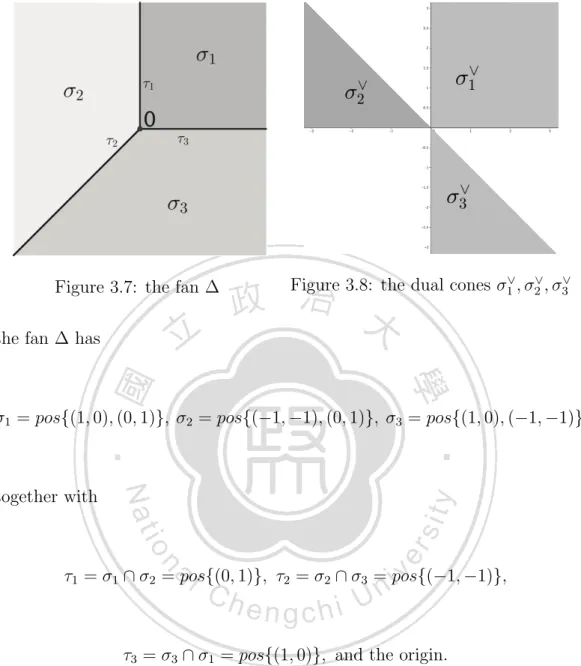
(51) varieties. According to Proposition 3.3.15, we have two embedding maps h1 : Uσ1 ∩σ2 �→ Uσ1 and h2 : Uσ1 ∩σ2 �→ Uσ2 . We define an equivalence relation by A ∼ B where A and B are in Uσ1 and Uσ2 respectively if and only if h1 ◦ h−1 2 (B) = A. Note that we have the following commutative diagram:. � Uσ1 ∩σ �� 2. � h2. �� Uσ. 2. h1 ◦h−1 2. h1. h2 ◦h−1 1. �. Uσ1. �. Definition 3.3.17. Given a fan ∆ in NR . We define the toric variety by the quotient space X∆ :=. �. �. σ∈∆. Uσ. �. �. ∼,. that is the disjoint union of the affine toric varieties, and ∼ is the above equivalence relation.. Next, the following example of the toric variety is over C. Albeit we will discuss the same case in the Example 4.3.2, it is over tropical semifield T. And we will know the difference between toric varieties and tropical toric varieties later. Example 3.3.18. Given the lattice N � Z2 , then NR = N ⊗ R � R2 , the dual lattice M � Z2 and MR = M ⊗ R. Let the fan ∆ in NR . Suppose that 43.

(52) Figure 3.7: the fan ∆. Figure 3.8: the dual cones σ1∨ , σ2∨ , σ3∨. the fan ∆ has. σ1 = pos{(1, 0), (0, 1)}, σ2 = pos{(−1, −1), (0, 1)}, σ3 = pos{(1, 0), (−1, −1)},. together with. τ1 = σ1 ∩ σ2 = pos{(0, 1)}, τ2 = σ2 ∩ σ3 = pos{(−1, −1)},. τ3 = σ3 ∩ σ1 = pos{(1, 0)}, and the origin. Then the dual cones. σ1∨ = pos{(1, 0), (0, 1)}, σ2∨ = pos{(−1, 0), (−1, 1)}, σ3∨ = pos{(1, −1), (0, −1)}.. 44.

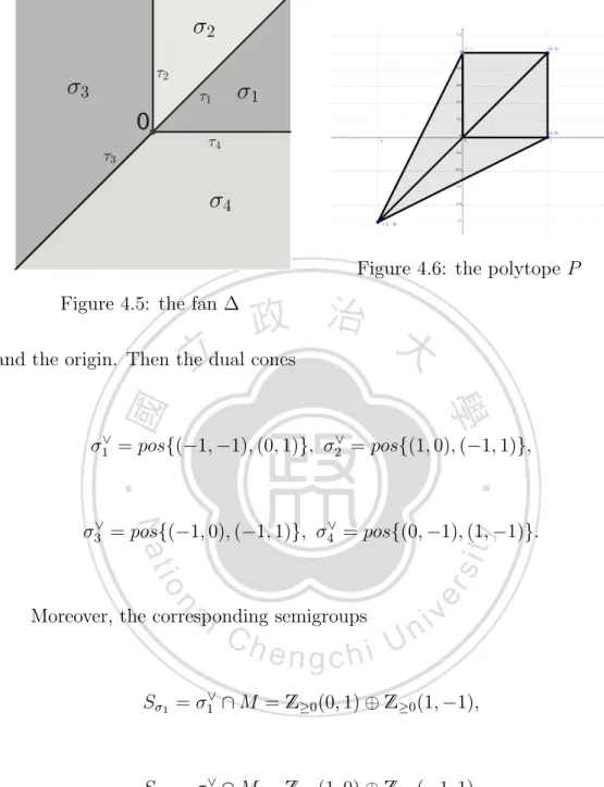
(53) Moreover, the corresponding semigroups. Sσ1 = σ1∨ ∩ M = Z≥0 (1, 0) ⊕ Z≥0 (0, 1),. Sσ2 = σ2∨ ∩ M = Z≥0 (−1, 0) ⊕ Z≥0 (−1, 1), Sσ3 = σ3∨ ∩ M = Z≥0 (1, −1) ⊕ Z≥0 (0, −1), together with. Sτ1 = Sσ1 + Sσ2 = Z≥0 (1, 0) ⊕ Z≥0 (−1, 0) ⊕ Z≥0 (0, 1),. Sτ2 = Sσ2 + Sσ3 = Z≥0 (1, −1) ⊕ Z≥0 (−1, 1) ⊕ Z≥0 (−1, −1), Sτ3 = Sσ3 + Sσ1 = Z≥0 (1, 0) ⊕ Z≥0 (0, 1) ⊕ Z≥0 (0, −1), S{0} = Z≥0 (1, 0) ⊕ Z≥0 (0, 1) ⊕ Z≥0 (−1, 0) ⊕ Z≥0 (0, −1).. Let x1 := χ(1,0) , x2 := χ(−1,0) , x3 := χ(0,1) and x4 := χ(0,−1) . Then x1 x2 = 1 and x3 x4 = 1, and we have. C[Sσ1 ] = C[x1 , x3 ], C[Sσ2 ] = C[x2 , x2 x3 ], C[Sσ3 ] = C[x1 x4 , x4 ],. C[Sτ1 ] = C[x1 , x2 , x3 ], C[Sτ2 ] = C[x1 x4 , x2 x3 , x2 x4 ], and C[Sτ3 ] = C[x1 , x3 , x4 ]. 45.

(54) Therefore, the affine toric variety. Uσ1 = hom(Sσ1 , C) � SpecC[Sσ1 ] = SpecC[x1 , x3 ] � C × C,. Uσ2 = hom(Sσ2 , C) � SpecC[Sσ2 ] = SpecC[x2 , x2 x3 ] � C × C, Uσ3 = hom(Sσ3 , C) � SpecC[Sσ3 ] = SpecC[x1 x4 , x4 ] � C × C, together with. Uτ1 = hom(Sτ1 , C) = C∗ × C, Uτ2 = hom(Sτ2 , C) = C∗ × C,. Uτ3 = hom(Sτ3 , C) = C∗ × C, U{0} = hom(S{0} , C) = C∗ × C∗ .. The gluing of the affine toric varieties Uσ1 and Uσ2 along their common subset Uτ1 gives CP2 with coordinates (z0 : z1 : z2 ) where x1 = z1 /z0 and x3 = z2 /z0 . The gluing of the affine toric varieties Uσ2 and Uσ3 along their common subset Uτ2 gives CP2 with coordinates (z0 : z1 : z2 ) where x2 x3 = z1 /z0 and x2 = z2 /z0 . The gluing of the affine toric varieties Uσ3 and Uσ4 along their common subset Uτ3 gives CP2 with coordinates (z0 : z1 : z2 ) where x3 = z1 /z0 and x1 = z2 /z0 .. 46.

(55) The following commutative diagram: Uσ 1 <. ⊃. Uτ1. ⊂. <. > Uσ2 ∧. ⊃. ∪. Uτ3. Uτ2. ⊂. ∩. >. ∨ Uσ3. Hence the gluing of these two gives the toric variety. X∆ (T) =. �. �. Uσ. σ∈∆. �. �. 2 ∼ = CP .. Theorem 3.3.19 (Hironaka’s Theorem). Let V be a quasi-projective variety. Then there exists a smooth quasi-projective variety X and a projective birational morphism π : X → V . Furthermore, π may be assumed to be an isomorphism on the smooth locus of V , and if V is a projective variety, then so is X.. Proof. See [25] p.106.. Let X = {(x, [p]) ∈ An × Pn−1 | x ∈ [p]} in An × Pn−1 . The blow − up of An at a point [p] is the map π : X → An via (x, [p]) �→ x.. 47.

(56) 3.4. Fano varieties. In this section, we will introduce and outline the Fano variety and Fano polytope. For more information see [5], [22], [7], [8] and [14]. Definition 3.4.1. For all r in Z, we define the Hirzebruch surface. Hr := {([x0 : x1 ], [y0 : y1 : y2 ]) ∈ CP1 × CP2 | xr0 y0 = xr1 y1 }.. Since Hr is isomorphic to H−r for all r in Z, we sometimes assume Z≥0 . Theorem 3.4.2. Let P ba a polytope in NR . If all of facets of P are the convex hull of a basis of N if and only if XP is a smooth Fano variety.. Proof. See [14] Proposition 3.6.7 and [7] Lemma 8.5.. The Fano varieties in two-dimension are also called a del Pezzo surface. Theorem 3.4.3. There exist five distinct toric Fano varieties of two-dimension up to isomorphism, 1. CP2 , 2. CP1 × CP1 , 3. the equivariant blowing-up of CP2 at one point (i.e. the Hirzebruch surface H1 ), 48.

(57) 4. the equivariant blowing-up of CP2 at two point, 5. the equivariant blowing-up of CP2 at three point.. Proof. See [22] Propsition 2.21.. 49.

(58) Chapter 4. Tropical Toric Variety. 4.1. K(G, R, M ). Definition 4.1.1. For all real number x, we define. x+ := max(x, 0),. x− := max(−x, 0), and called positive part and negative part of x, respectively. Remark 4.1.2. The x+ and x− are non-negative and x = x+ − x− . Definition 4.1.3. For all extended real-valued function f , the positive part 50.

(59) of f is defined by f + (x) := max{f (x), 0}, and the negaive part of f is defined by f − (x) := max{−f (x), 0}. So we have f = f + − f − . Remark 4.1.4. Let f := (f1 , · · · , fn ) ∈ R1×n , then f + = (f1+ , · · · , fn+ ), f − = (f1− , · · · , fn− ), and f = f + − f − . Proposition 4.1.5. Let f := (f1 , · · · , fn ) ∈ R1×n and x := (x1 , · · · , xn ) ∈ Rn , then the equations f · x = 0 if and only if f + · x = f − · x. Proof. Suppose that f · x = 0 where f := (f1 , · · · , fn ) ∈ R1×n and x := (x1 , · · · , xn ) ∈ Rn . Then (f1 , · · · , fn ) · (x1 , · · · , xn ) = 0 implies f1 × x1 + · · · fn × xn = 0. Since fi = fi+ − fi− for all i = 1, · · · , n, we have (f1+ − f1− ) × x1 + · · · + (fn+ − fn− ) × xn = 0. Therefore, f1+ × x1 + · · · + fn+ × xn = f1− × x1 + · · · + fn− × xn . Hence f + · x = f − · x. Conversely, assume that f + · x = f − · x where f + , f − ∈ R1×n and x := (x1 , · · · , xn ) ∈ Rn , then f1+ × x1 + · · · + fn+ × xn = f1− × x1 + · · · + fn− × xn . So we have (f1+ − f1− ) × x1 + · · · + (fn+ − fn− ) × xn = 0. Hence f · x = 0 since fi = fi+ − fi− for all i = 1, · · · , n and x := (x1 , · · · , xn ) ∈ Rn . Definition 4.1.6. Let S be a semigroup in Zn and let G = {g1 , · · · , gm } be a finite set of generators of S. Let R = {r1 , · · · , rk } ⊆ Zm generate the integer relation between a set of G, that is, SpanZ (R) = {z ∈ Zm | g1 z1 + · · · + gm zm = 0}. Let M be another commutative semigroup. We 51.

(60) define � � K(G, R, M ) := x ∈ M |G| | r+ · x = r− · x ∀r ∈ R We will discuss about that r · x = 0 is different from r+ · x = r− · x in the tropical semifield T. Example 4.1.7. Let S ⊆ Z2 and let G = {(1, 1), (4, 4)} be the generating set of S. Then |G| = 2, and we have (1, 1)z1 + (4, 4)z2 = 0 for all z1 , z2 ∈ Z. This implies R = {(−4, 1)} and SpanZ (R) = {(z1 , z2 ) ∈ Z2 | z1 + 4z2 = 0} Let M = T and let x = (x1 , x2 ) ∈ T2 . Then r · x = 0T where 0T is the tropical additive identity. This implies (−4 ⊙ x1 ) ⊕ (1 ⊙ x2 ) = 0T , so max{−4 + x1 , 1 + x2 } = −∞. Hence (x1 , x2 ) = (−∞, −∞). However, r+ · x = (0, 1) · (x1 , x2 ) = (0 ⊙ x1 ) ⊕ (1 ⊙ x2 ) = max{0 + x1 , 1 + x2 }. Similarly r− ·x = max{4+x1 , 0+x2 }. So {(x1 , x2 ) ∈ T2 | r+ · x = r− · x ∀r ∈ R} = {−∞, x1 + 3 = x2 }. Then K(G, R, T) = {−∞, x1 + 3 = x2 } Hence r · x = 0 is different from r+ · x = r− · x in T. Proposition 4.1.8. Given G = {g1 , . . . , gm }. Let R = {r1 , · · · , rk } ⊆ Zm Let M be a tropical semifield T. Suppose that K = K(G, R, T) = {x ∈ Tm | r+ · x = r− · x ∀r ∈ R}. We define two operations ⊕K : K × K → K and ⊗K : T × K → K by x ⊕K y = (x1 ⊕ y1 , . . . , xm ⊕ ym ) and t ⊗K x = (t⊙x1 , . . . , t⊙xm ), respectively. Then (K, ⊕K , ⊗K ) is a tropical vector space. 52.

(61) Proof. Let x = (x1 , . . . , xm ), y = (y1 , . . . , ym ), and v = (v1 , . . . , vm ) be in K, and let t, t1 , and t2 be in T. Given r = (z1 , . . . , zm ) is in R. Then r+ · x = r− · x and r+ · y = r− · y. We claim that K is closed under an operations ⊕K .. + r+ · (x ⊕K y) = (z1+ , . . . , zm ) · (x1 ⊕ y1 , . . . , xm ⊕ ym ) + = (z1+ ⊙ (x1 ⊕ y1 )) ⊕ · · · ⊕ (zm ⊙ (xm ⊕ ym )) + = (z1+ + max{x1 , y1 }) ⊕ · · · ⊕ (zm + max{xm , ym }) + + = max{z1+ + x1 , z1+ + y1 } ⊕ · · · ⊕ max{zm + xm , zm + ym } + + = ((z1+ ⊙ x1 ) ⊕ (z1+ ⊙ y1 )) ⊕ · · · ⊕ ((zm ⊙ xm ) ⊕ (zm ⊙ ym )) + + = ((z1+ ⊙ x1 ) ⊕ · · · ⊕ (zm ⊙ xm )) ⊕ ((z1+ ⊙ y1 ) ⊕ · · · ⊕ (zm ⊙ ym )). (since (T, ⊕) is a commutative monoid.) + + = ((z1+ , . . . , zm ) · (x1 , . . . , xm )) ⊕ ((z1+ , . . . , zm ) · (y1 , . . . , ym )). = (r+ · x) ⊕ (r+ · y) = (r− · x) ⊕ (r− · y) − − = ((z1− , . . . , zm ) · (x1 , . . . , xm )) ⊕ ((z1− , . . . , zm ) · (y1 , . . . , ym )) − − = ((z1− ⊙ x1 ) ⊕ · · · ⊕ (zm ⊙ xm )) ⊕ ((z1− ⊙ y1 ) ⊕ · · · ⊕ (zm ⊙ ym )) − − ⊙ xm ) ⊕ (zm ⊙ ym )) = ((z1− ⊙ x1 ) ⊕ (z1− ⊙ y1 )) ⊕ · · · ⊕ ((zm. (since (T, ⊕) is a commutative monoid.). 53.

(62) − − = max{z1− + x1 , z1− + y1 } ⊕ · · · ⊕ max{zm + xm , zm + ym } − = (z1− + max{x1 , y1 }) ⊕ · · · ⊕ (zm + max{xm , ym }) − = (z1− ⊙ (x1 ⊕ y1 )) ⊕ · · · ⊕ (zm ⊙ (xm ⊕ ym )) − = (z1− , . . . , zm ) · (x1 ⊕ y1 , . . . , xm ⊕ ym ). = r− · (x ⊕K y). Hence x ⊕K y is in K. We claim that K is closed under an operations ⊗K .. + r+ · (t ⊗K x) = (z1+ , . . . , zm ) · (t ⊙ x1 , . . . , t ⊙ xm ) + = (z1+ ⊙ (t ⊙ x1 )) ⊕ · · · ⊕ (zm ⊙ (t ⊙ xm )) + = ((z1+ ⊙ t) ⊙ x1 ) ⊕ · · · ⊕ ((zm ⊙ t) ⊙ xm ) (since (T, ⊙) satisfies associative.) + = ((t ⊙ z1+ ) ⊙ x1 ) ⊕ · · · ⊕ ((t ⊙ zm ) ⊙ xm ) (since (T \ {0T }, ⊙) is abelian.) + = (t ⊙ (z1+ ⊙ x1 )) ⊕ · · · ⊕ (t ⊙ (zm ⊙ xm )) + = t ⊙ ((z1+ ⊙ x1 ) ⊕ · · · ⊕ (zm ⊙ xm )) ( since (T, ⊕, ⊙) is a semifield.). = t ⊙ (r+ · x) = t ⊙ (r− · x) − = t ⊙ ((z1− ⊙ x1 ) ⊕ · · · ⊕ (zm ⊙ xm )) − = (t ⊙ (z1− ⊙ x1 )) ⊕ · · · ⊕ (t ⊙ (zm ⊙ xm )) (since (T, ⊕, ⊙) is a semifield.). 54.

(63) − = ((t ⊙ z1− ) ⊙ x1 ) ⊕ · · · ⊕ ((t ⊙ zm ) ⊙ xm ) (since (T \ {0T }, ⊙) is abelian.) − = ((z1− ⊙ t) ⊙ x1 ) ⊕ · · · ⊕ ((zm ⊙ t) ⊙ xm ) − = (z1− ⊙ (t ⊙ x1 )) ⊕ · · · ⊕ (zm ⊙ (t ⊙ xm )) (since (T, ⊙) satisfies associative.) − = (z1− , . . . , zm ) · (t ⊙ x1 , . . . , t ⊙ xm ). = r− · (t ⊗K x). Hence t ⊗K x is in K.. x ⊕K (y ⊕K v) = x ⊕K (y1 ⊕ v1 , . . . , ym ⊕ vm ) = (x1 ⊕ (y1 ⊕ v1 ), . . . , xm ⊕ (ym ⊕ vm )) = ((x1 ⊕ y1 ) ⊕ v1 ), . . . , (xm ⊕ ym ) ⊕ vm ) = (x1 ⊕ y1 , . . . , xm ⊕ ym ) ⊕K v = (x ⊕K y) ⊕K v. (0T , . . . , 0T ) ⊕K x = (−∞, . . . , −∞) ⊕K (x1 , . . . , xm ) = ((−∞) ⊕ x1 , . . . , (−∞) ⊕ xm ) = (x1 , . . . , xm ). 55.

(64) (t1 ⊙ t2 ) ⊗K x = ((t1 ⊙ t2 ) ⊙ x1 , . . . , (t1 ⊙ t2 ) ⊙ xm ) = (t1 ⊙ (t2 ⊙ x1 ), . . . , t1 (⊙t2 ⊙ xm )) = t1 ⊗K (t2 ⊙ x1 , . . . , t2 ⊙ xm ) = t1 ⊗K (t2 ⊗K x). (t1 ⊕ t2 ) ⊗K x = ((t1 ⊕ t2 ) ⊙ x1 , . . . , (t1 ⊕ t2 ) ⊙ xm ) = ((t1 ⊙ x1 ) ⊕ (t2 ⊙ x1 ), . . . , (t1 ⊙ xm ) ⊕ (t2 ⊙ xm )) = (t1 ⊙ x1 , . . . , t1 ⊙ xm ) ⊕K (t2 ⊙ x2 , . . . , t1 ⊙ xm ) = (t1 ⊗K x) ⊕K (t2 ⊗K x). t ⊗K (x ⊕K y) = t ⊗K (x1 ⊕ y1 , . . . , xm ⊕ ym ) = (t ⊙ (x1 ⊕ y1 ), . . . , t ⊙ (xm ⊕ ym )) = ((t ⊙ x1 ) ⊕ (t ⊙ y1 ), . . . , (t ⊙ xm ) ⊕ (t ⊙ ym )) = (t ⊙ x1 , . . . , t ⊕ xm ) ⊕K (t ⊙ y1 , . . . , t ⊕ ym ) = (t ⊗K x) ⊕K (t ⊗K y). Hence (K, ⊕K , ⊗K ) is a tropical vector space. Proposition 4.1.9. If M is a abelian group, then K(G, R, M ) is a abelian 56.

(65) group.. Proof. Let M be an abelian group with an operation ∗ : M × M → M by ∗(a, b) = a ∗ b. Then M |G| is also an abelian group. Because G is finite set, so we can consider |G| = k. We want to show that K(G, R, M ) is a subgroup of M k . Let x = (x1 , . . . , xk ) and y = (y1 , . . . , yk ) in K(G, R, M ). We claim that x ∗ y −1 = (x1 ∗ y1−1 , . . . , xk ∗ yk−1 ) in K(G, R, M ) where y −1 is the inverse for y. Since M is an abelian group, we have xi ∗ yi−1 in M for all i = 1, . . . , k, thus x ∗ y −1 in M k . Let r = (z1 , . . . , zk ) in SpanZ R. Since M is an abelian, M is a Z-module, thus (zi+ · (xi ∗ yi−1 )) = ((zi+ · xi ) ∗ (zi+ · yi−1 )) and (zi− · (xi ∗ yi−1 )) = ((zi− · xi ) ∗ (zi− · yi−1 )) for all i = 1, . . . , k. Moreover, r+ · x = r− · x and r+ · y −1 = r− · y −1 , because x = (x1 , . . . , xk ) and y = (y1 , . . . , yk ) in K(G, R, M ). So we have. r+ · (x ∗ y −1 ) = (z1+ , . . . , zk+ ) · (x1 ∗ y1−1 , . . . , xk ∗ yk−1 ) = (z1+ · (x1 ∗ y1−1 )) ∗ · · · ∗ (zk+ · (xk ∗ yk−1 )) = ((z1+ · x1 ) ∗ (z1+ · y1−1 )) ∗ · · · ∗ ((zk+ · xk ) ∗ (zk+ · yk−1 )) = ((z1+ · x1 ) ∗ · · · ∗ (zk+ · xk )) ∗ ((z1+ · y1−1 ) ∗ · · · ∗ (zk+ · yk−1 )) = r+ · x ∗ r+ · y −1 = r− · x ∗ r− · y −1. 57.

(66) = ((z1− · x1 ) ∗ · · · ∗ (zk− · xk )) ∗ ((z1− · y1−1 ) ∗ · · · ∗ (zk− · yk−1 )) = ((z1− · x1 ) ∗ (z1− · y1−1 )) ∗ · · · ∗ ((zk− · xk ) ∗ (zk− · yk−1 )) = (z1− · (x1 ∗ y1−1 )) ∗ · · · ∗ (zk− · (xk ∗ yk−1 )) = (z1− , . . . , zk+ ) · (x1 ∗ y1−1 , . . . , xk ∗ yk−1 ) = r− · (x ∗ y −1 ).. Hence we get x ∗ y −1 in K(G, R, M ), i.e. K(G, R, M ) is a group. Next we claim that K(G, R, M ) is an abelian. Suppose that x = (x1 , . . . , xk ) and y = (y1 , . . . , yk ) in K(G, R, M ). Since M is an abelian, xi ∗ yi = yi ∗ xi for all i = 1, . . . , k. Then. x ∗ y = (x1 , . . . , xk ) ∗ (y1 , . . . , yk ) = (x1 ∗ y1 , . . . , xk ∗ yk ) = (y1 ∗ x1 , . . . , yk ∗ xk ) =y∗x. Hence K(G, R, M ) is an abelian group.. By the above proposition, K(G, R, T \ {−∞}) is an abelian group since (T \ {−∞}, ⊙) is an abelian group.. 58.

(67) Example 4.1.10. Let S ⊆ Z2 and let G = {(1, 2), (2, 4)} be the generating set of S. Then |G| = 2, and we have (1, 2)z1 + (2, 4)z2 = 0 for all z1 , z2 ∈ Z. This implies R = {r = (−2, 1)}. So r+ = (0, 1) and r− = (2, 0). Given an abelian group M = (Z4 , +). Let x = (x1 , x2 ) ∈ Z4 × Z4 . If r+ · x = r− · x, then x2 = 2x1 , and so K(G, R, Z4 ) = {(x1 , x2 ) ∈ Z4 × Z4 | x2 = x1 } is subset of Z4 × Z4 . We claim that K(G, R, Z4 ) is a subgroup of Z24 . Suppose that (x1 , x2 ) and (y1 , y2 ) are in K(G, R, Z4 ), then x2 = 2x1 and y2 = 2y1 . Then 2(x1 +(−y1 )) = 2x1 + 2(−y1 ) = 2x1 + (−2y1 ) = x2 + (−y2 ) where (−y1 , −y2 ) is the inverse element of (y1 , y2 ), so (x1 + (−y1 ), x2 + (−y2 )) is in K(G, R, Z4 ). Since xi + yi = yi + xi for all i = 1, 2, (x1 , x2 ) + (y1 , y2 ) = (x1 + y1 , x2 + y2 ) = (y1 + x1 , y2 + x2 ) = (y1 , y2 ) + (x1 , x2 ) Hence K(G, R, Z4 ) is abelian group. Proposition 4.1.11. If M is a ring, then K(G, R, M ) is a M -module.. Proof. Suppose that M is a ring with binary operation ∗, together with a second binary operation ⊗. Because (M, ∗, ⊗) is a ring, so (M, ∗) is an abelian group, thus K(G, R, M ) is also an abelian group. Define a operation � : K(G, R, M ) × M → K(G, R, M ) via x � m = (x1 ⊗ m, . . . , xk ⊗ m). To check that it is well-defined. Suppose that r is in R and |G| = k. Let m, n be in M and let x = (x1 , . . . , xk ), y = (y1 , . . . , yk ) in 59.

(68) K(G, R, M ). Then r+ · x = r− · x.. r+ · (x � m) = (z1+ , . . . , zk+ ) · (x1 ⊗ m, . . . , xk ⊗ m) = z1+ ⊗ (x1 ⊗ m) ∗ · · · ∗ zk+ ⊗ (xk ⊗ m) = (z1+ ⊗ x1 ) ⊗ m ∗ · · · ∗ (zk+ ⊗ xk ) ⊗ m = (z1+ ⊗ x1 , . . . , zk+ ⊗ xk ) � m = (r+ · x) � m = (r− · x) � m = (z1− ⊗ x1 , . . . , zk− ⊗ xk ) � m = (z1− ⊗ x1 ) ⊗ m ∗ · · · ∗ (zk− ⊗ xk ) ⊗ m = z1− ⊗ (x1 ⊗ m) ∗ · · · ∗ zk− ⊗ (xk ⊗ m) = (z1− , . . . , zk− ) · (x1 ⊗ m, . . . , xk ⊗ m) = r− · (x � m). So x � m is in K(G, R, M ). Suppose that x = y (i.e. xi = yi for all i = 1, . . . , k) and m = n, then x � m = (x1 ⊗ m, . . . , xk ⊗ m) = (y1 ⊗ n, . . . , yk ⊗ n) = y � n. Hence it is well-defined.. (x ∗ y) � m = (x1 ∗ y1 , . . . , xk ∗ yk ) � m 60.

(69) = ((x1 ∗ y1 ) ⊗ m, . . . , (xk ∗ yk ) ⊗ m) = ((x1 ⊗ m) ∗ (y1 ⊗ m), . . . , (xk ⊗ m) ∗ (yk ⊗ m)) = (x1 ⊗ m, . . . , xk ⊗ m) ∗ (y1 ⊗ m, . . . , yk ⊗ m) = (x � m) ∗ (y � m). x � (m ∗ n) = (x1 , . . . , xk ) � (m ∗ n) = (x1 ⊗ (m ∗ n), . . . , xk ⊗ (m ∗ n)) = ((x1 ⊗ m) ∗ (x1 ⊗ n), . . . , (xk ⊗ m) ∗ (xk ⊗ n)) = (x1 ⊗ m, . . . , xk ⊗ m) ∗ (x1 ⊗ n, . . . , xk ⊗ n) = (x � m) ∗ (x � n). (x � m) � n = (x1 ⊗ m, . . . , xk ⊗ m) � n = ((x1 ⊗ m) ⊗ n, . . . , (xk ⊗ m) ⊗ n) = (x1 ⊗ (m ⊗ n), . . . , xk ⊗ (m ⊗ n)) = x � (m ⊗ n). If M has an identity 1M , that is m ⊗ 1M = m for all m ∈ M . Then x � 1M = (x1 ⊗ 1M , . . . , xk ⊗ 1M ) = (x1 , . . . , xk ) = x. 61.

(70) Remark 4.1.12. If M is a field, then K(G, R, M ) is a vector space. Example 4.1.13. Let M = GF (4) be a Galois field. Let S ⊆ Z2 and let G = {(1, 2), (4, 8)} be the generating set of S. Then |G| = 2, and we have (1, 2)z1 + (4, 8)z2 = 0 for all z1 , z2 ∈ Z. This implies R = {r = (−4, 1)}. So r+ = (0, 1) and r− = (4, 0). If r+ · x = r− · x where x = (x1 , x2 ) is in GF (4)2 , then x2 = 4x1 = 0, and so K(G, R, GF (4)) = {(x1 , x2 ) ∈ GF (4)2 | x2 = 0} is a subset of GF (4)2 . We claim that K(G, R, GF (4)) is a vector space, in fact, we just need to show that K(G, R, GF (4)) is a subspace of GF (4)2 . To start with, it is clearly that (0, 0) is in K(G, R, GF (4)). Next, suppose that x = (x1 , x2 ) and y = (y1 , y2 ) are in K(G, R, GF (4)), then x2 = 0 and y2 = 0, then x2 +y2 = 0, and so x+y is in K(G, R, GF (4)). Finally, let c be in GF (4), and let x = (x1 , x2 ) be in K(G, R, GF (4)), then x2 = 0 and cx = (cx1 , cx2 ), then cx2 = 0, and so cx is in K(G, R, GF (4)). Hence K(G, R, GF (4)) is a subspace of GF (4)2 . � Note that the Galois field GF (4) is isomorphic to GF (2) (x2 + x + 1),. in fact GF (2) � Z2 since GF (p) � Zp for all prime p.. Theorem 4.1.14. Let S be a finitely generated semigroup on Zn . Let G = {g1 , · · · , gl } be a set of generaters with relations generated by R = {r1 , · · · , rk }. Let M be an additive semigroup. Then there is a bijection between hom(S, M ) and K(G, R, M ). 62.