Final Report of Research Project
of
National Science Council
Kuroshio Intrusion in Luzon Strait
黑潮於呂宋海峽的入侵
By
T. Y. Tang
唐存勇
Institute of Oceanography
National Taiwan University
Taipei, Taiwan, ROC
Research Project No: NSC 89-2611-M-002-031-OP2
1. 簡介
在計畫書中承諾以蒐集的海洋資料配合數值式研究探討黑潮於呂
宋海峽的入侵及其在北南海的行為。研究執行尚稱亦好,撰寫一篇論
文–Kuroshio Intrusion in Luzon Strait,目前已送至 Journal of Physical
Oceanography 審查,二審查人皆建議接受但須要一定程度的修改。另
外亦完成一篇有關黑潮與北南流的作用結果,文章名為
“Intra-seasonal variation in the velocity field of the northeastern South
China Sea”,文章已運 Geophysical Research Letter 審查中。計畫主
持人另有數篇 papers,或已接發表,或正在 in press,或仍在審查修
正中,但因這些 papers 與此計畫無直接關連,故未列入此報告中。
第 2 章將二篇論文陳列做為此計畫的成果,第 3 章將討論結果的
2. 結果
Kuroshio Intrusion in the Luzon Strait
By
T. Y. TANG1, W.-D LIANG2, Y. J. YANG3, and W.-S. CHUANG1
1
Institute of Oceanography, National Taiwan University, Taipei, Taiwan, ROC
2
National Center for Ocean Research, Taipei, Taiwan, ROC
3
Department of Marine Science, Chinese Naval Academy, Tsoying, Kaohsiung, Taiwan, ROC
Submitted to Journal of Physical Oceanography
ABSTRACT
Three Acoustic Doppler Current Profilers (ADCP) were deployed in the central
Luzon Strait to monitor current velocity. The duration of deployment varied with
location and spanned from 1997 to 1999. The observed current velocity indicated
that the Kuroshio consistently intruded into the South China Sea. The current
velocity demonstrated small annual variation, but large intraseasonal variation. The
change of monsoons, from northeast to southwest, did not cause noticeable variation
in current velocity.
The Miami Isopycnic Coordinate Ocean Model (MICOM) forced by the wind
data provided by the European Centre for Medium-Range Weather Forecasts
(ECMWF) was used to interpret the observed current velocity. Comparison between
the model output and observation validates the use of the model result in interpreting
annual and interannual current velocity variation in the Luzon Strait. The numerical
model result also shows that the Kuroshio consistently intruded into the South China
Sea, displaying a noticeable annual variation in the central Luzon Strait. The large
interannual variation masked the annual variation so that the annual variation was
difficult to observe. The interaction between the Kuroshio and the South China Sea
cyclonic flow caused the current velocity variation in the both the Luzon Strait and
loop current intrusion and confines to the northern South China Sea. In winter, the
Kuroshio can intrude deeply into the South China Sea, besides intruding as loop
current intrusion in the northern South China Sea.
The annual transport variation across the Luzon Strait is primarily westward.
The eastward transport was found in summer during certain years when the Kuroshio
intrusion was weak. In spite of the fact that the Kuroshio intruded consistently into
the South China Sea, transport out of the South China Sea was observed. In summer,
the current on the northern South China Sea shelf break contributed to the transport
out. The variation in zonal transport was caused by the Sea Surface Height (SSH)
variation occurring west of northern Luzon. Wind stress curl is responsible for this
1. Introduction
The Luzon Strait is located between Taiwan and Luzon. It is the primary
channel for exchanging water between the South China Sea and the North Pacific
Ocean. The width of the Luzon Strait, from southern Taiwan to northern Luzon, is
around 350 km. It is shallow at both the northern and southern ends and is deep in
the central portion. The maximum water depth is over 2500 m. The topography is
generally complicated in and around the Strait. A number of small islands are
located at the southern end of the Luzon Strait. The water depth increases rapidly to
the east and west of the Strait, where it meets the basins of the northern Pacific and
South China Sea. A shelf break occurs northwest of the Luzon Strait, where the
Taiwan Strait joins the South China Sea and the East China Sea. The current in the
Luzon Strait might affect the flow in the Taiwan Strait and possibly even the East
China Sea.
The Luzon Strait is the first large meridional gap for the principal North Pacific
Western Boundary Current (the Kuroshio). Whether the northward Kuroshio leaps
across the Luzon Strait or intrudes into the South China Sea through the Luzon Strait
is an issue that has often drawn oceanographers’ attention. Wyrtki (1961) and Nitani
(1972) suggested that the Kuroshio intruded into the South China Sea when the
This seasonal intrusion feature was re-confirmed by many scientists. Levitus (1982)
studied the Volunteer Observing Ship data (VOS); Shaw (1991) analyzed historical
hydrographic measurements, and Farris and Wimbush (1996) examined
satellite-derived Sea Surface Temperature (SST) images. All reached a similar
conclusion; Kuroshio intrusion occurs seasonally. Shaw and Chao (1994) forced a
numerical model based on the monthly climatological wind and also re-produced the
above findings. Nevertheless, a few studies obtained different results. For example,
Chu (2000) used the climatological hydrographic data to estimate intruded Kuroshio
transport in the Luzon Strait. The transport varied seasonally, but was consistently
westward, with the largest amount 13.7 Sv in February and the smallest amount 1.4
Sv in September. Using the historical temperature profiles, Qu (2000) obtained
similar results; the transport was westward consistently, but with different estimated
amounts of transport. The largest intruded volume was 5.3 Sv in January through
February and the smallest intruded volume was 0.2 Sv in June through July. The
numerical model produced by Metzger and Hurlburt (1996) displayed the features
stated in the findings of Qu (2000).
The mechanisms causing Kuroshio intrusion have also been a subject of
controversy. Stommel and Arons (1960) claimed that the western boundary current
(2001) indicated that the western boundary current could leap across the meridional
gap when the gap is small or the inertia is large. He inferred that the Kuroshio
intruded into the South China Sea in the season of northeast monsoon because the
speed of the Kuroshio was weakened by the head wind. Analyzing the hydrographic
measurements, Wang and Chern (1987) postulated that the Ekman transport, induced
by the monsoon, could be important for Kuroshio intrusion. The current in the South
China Sea could also be a factor affecting Kuroshio intrusion (Shaw and Chao, 1994).
Qu (2000) and Metzger and Hurlburt (1996) concluded that Kuroshio intrusion in the
Luzon Strait was primarily related to the meridional pressure gradient across the Strait.
All of these controversies are primarily the result of insufficient data, especially in
long-term moored current velocity measurements.
Liang et al. (2002) presented a composite current velocity, which was obtained
from 10 years of Ship-board Acoustic Doppler Current Velocity Profilers (Sb-ADCP),
positioned around Taiwan. The data revealed that the Kuroshio intruded into the
South China Sea through the central Luzon Strait. The volume transport in the upper
300 m water column across the Strait was 3.3 Sv westwardly. The intruded
Kuroshio interacted with the current in the South China Sea, forming a complicated
spatial distribution west of the Luzon Strait. Liang et al. (2002) produced a few
Kuroshio intrusion might be constant. Similar, but more complete moored current
velocity measurements are presented in this paper to study Kuroshio intrusion. The
moored current velocities are used to examine the validation of outputs of the Miami
Isopycnic Coordinate Ocean Model (MICOM; Bleck and Smith 1990; Bleck et al.
1992; Bleck and Chassignet 1994), which was forced by the European Centre for
Medium-Range Weather Forecasts [ECMWF (1995)] wind. Using the model
outputs, the factors causing Kuroshio intrusion are investigated. Since only monthly
wind data was applied, the studies focus on the annual and interannual variations of
Kuroshio intrusion in the Luzon Strait. This paper proceeds as follows. In Section
2, the moored current velocity in the Luzon Strait is presented. The Kuroshio
intrusion is described. In Section 3, the scheme of the numerical model is stated and
the observation and model output comparison is shown. The validation of model
outputs is discussed. Section 4 states the annual and interannual evolutions of
Kuroshio intrusion. The mechanisms causing such evolutions are examined. A
discussion and summary are provided in Section 5.
2. Observation
Figure 1 shows the locations of 3 moorings (named L1, L2, and L3), their
around Taiwan. The asterisk indicates Lanyu Island, where the wind record was
used. The moorings were located in the central portion of the Luzon Strait. L1 and
L3 were 120 km away from the tips of southern Taiwan and northern Luzon,
respectively. L2 is located between them. Moorings were located about 50 km
from each other. The water depth at L2 was deepest (over 2000 m), with L1 and L3
depths of around 1300 m and 1650 m, respectively. The composite current velocities,
adopted from Liang et al. (2002), indicate that L1 and L2 were located on the main
path of Kuroshio intrusion, while L3 was positioned near the southern intrusion
boundary. The duration of deployments varied with location. A few
refurbishments had to be made during deployment. Table 1 lists the start and ending
times, the depth of the instrument position, and local water depths for each
deployment. The moorings in the Luzon Strait had a large vertical excursion,
especially at L2, where the vertical excursion was occasionally greater than 200 m.
The large vertical excursion was primarily caused by the high tidal current speed.
The tidal current speed (recorded by VACM current meter and not shown) at 1100 m
was nearly 100 cm s-1 during spring tide. An attempt was made to increase
floatation in order to keep the mooring line upright. The mooring line broke and one
mooring was lost. Fortunately, all of the moorings had small pitching and rolling
ADCP was kept at a much shallower depth than the range (around 300 m) of the
narrow-band ADCP. The design, in combination with the ADCP range being larger
than the monitor range, made it possible to record the upper layer current velocities
simultaneous with the depth correction. A SEACAT CTD was mounted immediately
beneath the ADCP. It provided pressure data, which was used for the depth
correction. Short time gaps occasionally occurred at the uppermost depths and were
interpolated linearly. Fluctuations of horizontal speed caused by the vertical
excursions were estimated. Assuming that the maximum vertical excursion was 300
m, the ADCP moved horizontally about 1054 m over half of the semidiurnal tidal
period (6.21 hours) at a location where water depth was 2000 m. The estimated
maximum horizontal speed caused by the vertical excursion was less than 10 cm s-1.
It would not significantly bias the large subtidal current velocity in the Luzon Strait.
Figure 2 shows the eastward (U) and northward (V) components of current
velocity at L1, where water depth is 1300 m. The depth (30-220 m) average of U, V,
and their velocity sticks time series are also shown. The time series was low-pass
filtered to remove the fluctuations for frequencies higher than 0.0139 cycles per hour
(cph). The data covers a period of 1.5 months in 1997 and nearly 12 months
beginning April 1998. Westward velocity dominated in U. Eastward current was
(maximum around 70 cm s-1) at the surface and gradually decreased with depth (the
decreasing rate about 0.6 cm s-1 every 10 m). The seasonal change was vague. The
transition of monsoons usually occurred in April and September (Chuang and Liang
1994) and had no significant impact on the U. Northward current dominated in the V.
Southward current was rarely observed. The greatest V (maximum over 110 cm s-1)
occurred at the uppermost depth, decreasing with increasing depth (the decreasing rate
about 1.4 cm s-1 every 10 m). The V at depths below 200 m was generally less than
20 cm s-1. The V was weak from December through February when the northeast
monsoon gained full strength. The depth-averaged time series showed that the U
and V fluctuated, but their variance spectra (not shown) had no significant peak in the
specific frequency band. In general, the U had smaller amplitude than V. In a
peak-to-peak comparison, the north and east component velocities frequently varied
out of phase. The velocity sticks showed that the current at L1 moved primarily to
the north-northwest, but was more westward as velocity stick amplitude decreased.
The impact of typhoon on the current velocity was not clear. For example, the super
Typhoon, Zeb (minimum surface pressure of 880 mbar), moved almost exactly along
the mooring array in the Luzon Strait from south to north on October 14-16 of 1998.
It only induced short-term velocity fluctuations in the upper ocean, and can be barely
The low-pass filtered U and V at L2 are shown in Fig. 3. L2 is near the center
of the Luzon Strait where the water is deep (around 2200 m). The ADCP was
mounted at depths of 130 and 160 m for the two deployments in 1997, respectively.
These depths were shallower than the range of the ADCP. The rationale for keeping
the ADCP at shallow depth was explained above. Due to a mistake in mooring line
length, the ADCP was deployed at deeper depths in 1998. The range of available
current velocity was from 130 to 280 m. Nearly 9 months of current velocity data,
obtained in 1997, was used to describe the upper ocean current velocity at L2. The
current velocity obtained in 1998 was used as a reference. Like the current at L1, U
and V at L2 were dominated by the westward and northward component velocities,
respectively. Eastward and southward component velocities were rarely observed.
The maximum speed was around 100 cm s-1 for both westward and northward
component velocities. The greatest velocity occurred in the uppermost layer,
decreasing with depth (the decreasing rate about 1.0 cm s-1 every 10 m). The
depth-averaged U and V had similar amplitudes. The current flowed primarily
northwest, which was more westward than the current at L1. Peak-to-peak
comparison indicated that the variations of V and U were frequently out of phase.
Although the recorded velocity time series was shorter than a year, it covered the
difference was found. For example, the velocity in January through February, when
the northeast monsoon was dominant, showed little difference from the velocity in
May through July, when the southwest monsoon prevailed. The variance spectra of
U and V showed no distinctive peak at any specific frequency band. The current
fluctuated with various time scales. The velocity sticks indicated that the current
usually flowed toward the northwest. The deeper current velocity, measured in 1998,
was more northward than the shallower current velocity, measured in 1997. This
dissimilarity might be caused by the difference in depth.
Figure 4 shows the low-pass filtered U and V at L3. The current velocity at L3
had quite different characteristics than it did at L1 and L2. The U was weak
(maximum speed around 50 cm s-1 and decreasing rate about 0.6 cm s-1 every 10 m)
and changed its sign repeatedly. The V, dominated by northward velocity, was also
weaker (maximum speed less than 80 cm s-1 and decreasing rate about 0.7 cm s-1
every 10 m) than it was at the previous two stations. No seasonal preference was
observed in either U or V. For all of the nearly 9-month record, the mean of U was
near zero, while the mean of V was about 11 cm s-1 (northward). The depth (30-160
m) averaged current fluctuated with different time scales and different directions.
However, the current was northward more often than not.
current velocity spatial distribution in the Luzon Strait, a conclusion can be drawn.
The Kuroshio intruded consistently into the South China Sea through the central
Luzon Strait. It had small annual variations. L1 and L2 were located in the main
path of the Kuroshio intrusion. L3 appears to be a southern boundary of Kuroshio
intrusion where the Kuroshio intrusion was frequently observed to change to South
China Sea outflow. Figure 5 shows the T-S diagrams at L1, L2, L3, the South China
Sea and the upstream Kuroshio. An average of 5 CTD measurements (marked by
asterisk in Fig. 5) west of Luzon represents the South China Sea water. An average
of 3 CTD measurements (marked by cross in Fig. 5) northeast of Luzon represents the
upstream Kuroshio. The Kuroshio was saltier and warmer than the South China Sea
in the upper water column, but was less salty and colder in the lower water column.
Two T-S curves intersected at σt = 25.66. The T-S curve at L3 was close to the South China Sea, but gradually moved closer to the curve of Kuroshio water as the
location moved north. This finding provides extra evidence that L3 could be the
southern boundary of the intruded Kuroshio. However, the T-S curves at 3 stations
were notably different than T-S curves from the South China Sea and the Kuroshio.
This result implies that the Kuroshio and South China Sea water mix vigorously in the
Luzon Strait. The intense current could cause the water mixing.
1997 is shown in Fig. 6. The positive/negative wind velocity flows to the
northeast/southwest. The depth-average current velocity of U and V at L2 are also
shown. Overall coherences (not shown) between the current and wind velocities
were generally low. However, the peak-to-peak comparison shows that the current
fluctuation coincided occasionally with wind fluctuation. For example, the large
southwesterly wind oscillation in early June corresponded to the variations in both U
and V. Similar features were also found at L1 and L3, indicating that the local wind
played a role, but not the only one.
3. Numerical model
a. Model description
The MICOM model was applied in the numerical simulation. It is a primitive
equation numerical model that describes the evolution of momentum, mass, heat, and
salt in the ocean, configured with realistic topography and stratification. In contrast
to the traditional vertical coordinate of water depth in the level model, MICOM uses
equations that have a coordinate of density in the vertical direction. The advantage
of a layer model using density coordinate is that the system suppresses the diapycnal
component of numerically caused dispersion of material and thermodynamic
warming of deep-water masses, as has been shown to occur in level model
applications (Chassignet et al. 1996).
The model domain includes the western Pacific and the South China Sea with
boundaries at 20.8°S, 45.1°N and 95°E, 160°E (Fig. 7). The horizontal grid is
defined on a Mercator projection with resolution given by 1/4° × 1/4°cosφ (meridional × zonal), where φ is the latitude. The vertical density structure has 15 isopycnic layers, topped by a Kraus-Turner mixed layer (Kraus and Turner 1967). The
topography was interpolated from the ETOPO5 dataset (NOAA 1988). The model is
spun up for 10 years from rest; with an initial thermohaline condition interpolated
from the 1994 World Ocean Atlas (WOA94) (Levitus and Boyer 1994; Levitus et al.
1994) January temperature and salinity data. The model was forced by the
climatological monthly atmospheric momentum, heat and freshwater flux. The
momentum flux was calculated from 1985-1999 wind data provided by the ECMWF
with the drag coefficient described in Trenberth et al. (1989). The heat flux,
evaporation and precipitation were taken from the Comprehensive Ocean-Atmosphere
Data Set (COADS) (da Silva et al. 1994). The layer thickness, temperature and
salinity were relaxed to the climatology of the WOA94 monthly data in a 4° buffer
zone at the borders of model domain. This 10-year spin up model was continuously
flux were still forced by the climatology.
b. Observation and model comparison
Figure 8 shows the comparison between the observation and model output of
monthly average current velocity vectors at various depths and locations. The
agreement between model output and observation was good at L1, fair at L2, and poor
at L3. The two velocities at L1 were almost identical in direction, but the observed
current velocity had slightly larger amplitude than the model. At L2, good
agreement was also found in the upper 100 m water columns in 1997. The model
output velocity was only slightly more westward than the observed velocity. In the
lower water column (130-240 m) in 1998, the two current velocities had noticeable
differences in direction. The model output velocity was more westward. At L3,
the direction difference between the two velocities became more pronounced. The
observed current was primarily northward while the model output velocity was
principally northwestward. Although the difference between the two velocities at L3
was noteworthy, for both, the speed was smaller than it was at L1 and L2. L3 is
close to the margin of Kuroshio intrusion.
The comparison between model output and observed depth-averaged velocity
applied to both observation and model output. In general, the model output and
observation agree well in the low frequency variations at L1 and L2. Fluctuations
with time scales of several days to months, were large in the observed velocity, but
were not found in the model output. This could be related to the fact that the coarse
grid and monthly wind were applied to the model. The mean velocities, calculated
from model and observation, are nearly the same. Only slight differences were
found in V at L1 and U at L2. The annual variation was small for both model and
observed velocities. Even with the assistance of model output, such small annual
variation was not easily discernible. At L3, the model and observation had good
agreement in the low frequency variation of V, but not U. The mean of observed U
was nearly zero, while the mean of modeled U was -27 cm s-1. In the model output,
the Kuroshio consistently intruded into the South China Sea through L3. This
disagreement could be due to the fact that islands in the southern Luzon Strait were
not adequately represented in the model.
The above comparison both validates and limits the use of model output. Good
agreement in low frequency variation allows us to use the model output to study
annual and interannual variations. Conversely, the fact that model output lacks high
frequency variations prohibits its use for study of the intraseasonal variation, observed
c. Model output
The current velocity distributions at 50 m depth in June and December obtained
from the 10th year spin up model outputs in the region of 105°-130°E, 5°-25°N are
shown in Fig. 10. The Sea Surface Height (SSH) of the model output is also shown.
In June, the westward North Equatorial Current (NEC) in the western Pacific was
located primarily in the region of 10°-17°N. It separated into the northward
Kuroshio and southward Mindanao Current around 13°N as it approached Mindanao.
The Kuroshio flowed primarily northward along the eastern coast of the Philippines,
bending into the Luzon Strait, after leaving Luzon, but not immediately after. The
inertia effect might keep the swift Kuroshio flowing in its original direction when it
first leaves its western continental boundary. Meanwhile, the eastward current in the
southern Luzon Strait might prevent the Kuroshio from immediately intruding into the
South China Sea. The eastward current originates from the central or southwestern
South China Sea. A cyclonic flow, with double or tripe low-pressure (low SSH)
centers, was observed west of the Luzon Strait. This cyclonic flow varied seasonally.
It was weak and primarily confined to the northern South China Sea during the
southwest monsoon season, while it was strong and became a basin-wide feature
as South China Sea cyclonic flow. In the Luzon Strait, the Kuroshio separates into
two branches. One branch curves slightly clockwise and then flows primarily
northward and leaps across the Luzon Strait. The other branch intrudes into the
South China Sea and gradually merges and then cycles with the South China Sea
cyclonic flow. Only a small portion of the Kuroshio spilled over the shelf and
entered the Taiwan Strait. The current in the Taiwan Strait primarily originated from
the northern South China Sea shelf break or even further south, from the eastern
boundary of Vietnam.
The main feature of Kuroshio intrusion in December was similar to that in June,
but with some noticeable differences. In December, the region of NEC greatly
expanded northward and the origination of the Kuroshio moved slightly northward.
The surface current velocity distributions, obtained from the World Ocean Circulation
Experiment/Tropical Oceans Global Atmosphere (WOCE/TOGA) drifting buoys
(Hansen and Poulain, 1996), also revealed the feature of seasonal
expansion/contraction of the NEC in the western Pacific. The westward NEC
reached the northern tip of Luzon. The Kuroshio immediately curves to the
northwest, as it leaves Luzon. It again separates into two branches in the Luzon
Strait. One leaps across the Strait. The other branch intrudes into the South China
this cyclonic flow, included a stronger meso-scale cyclonic flow in northeastern
section and a weaker one in the southwest section, is nearly basin-wide. A strong
low-SSH appears west of northern Luzon and southern Luzon Strait. The intruded
Kuroshio flows primarily with the South China Sea cyclonic flow into the central and
southern South China Sea. A small portion of the intruded Kuroshio curves
clockwise, flowing along the southern opening of Taiwan Strait. It either enters the
Taiwan Strait or flows out through the southern tip of Taiwan added to the Kuroshio.
The current on the northern South China Sea shelf break is weaker in December than
in June. The Kuroshio becomes an important source for current in the Taiwan
Strait in December. It is noteworthy that the meridional gradient of the SSH across
the Luzon Strait is larger in December than in June.
In Fig. 10, it is also shown that the Luzon Strait is not the only opening in the
South China Sea. Besides, the South China Sea circulation system is mainly driven
by the monsoon. It causes that the Kuroshio in the Luzon Strait differs from the loop
current of Gulf Stream in the Gulf of Mexico. The cyclonic flow west of the Luzon
Strait confined the loop current in the northern South China Sea. And due to the
shallow water of the continental shelf southeast of China, the bottom friction causes
that the eddy is seldom shedding from the loop current and less than 100 km in length
the Luzon Strait, the Mindanao Current in the Sulawesi Sea is more similar to the loop
current of Gulf Stream in the Gulf of Mexico. The eddy is often shedding from loop
current and more than 300 km in length scale. The shedding eddy is moving
westwardly and deceasing in the western Sulawesi Sea.
In general, the Kuroshio only intrudes as a loop current intrusion and confines to
the northern South China Sea in summer. In winter, the Kuroshio can intrude
deeply into east of Vietnam, besides intruding as loop current intrusion in the northern
South China Sea.
4. Kuroshio Intrusion
a. Current around the Luzon Strait
Focusing on Kuroshio intrusion, Figure 11 shows the current velocity
distributions at 50 m and SSH around the Luzon Strait. The figure contains 20
panels, 5 rows by 4 columns. Four columns, from top to bottom, represent the
current velocity on 15th of March, June, September and December, while 5 rows,
from left to right, represent years 1997, 1998, 1999, 2000, and 2001. The current
velocity distributions in 1997 are used to illustrate the annual evolution. The
greatest Kuroshio intrusion into the South China Sea occurred in March. The South
China Sea cyclonic flow with strong low SSH center was found immediately west of
cyclonic flow. A small portion of the Kuroshio spilled out, entering the Taiwan
Strait. In June, the Kuroshio consistently intruded into the South China Sea and
merged with the cyclonic flow. However, when the South China Sea cyclonic flow
was weak and shifted to the west, the strength of the Kuroshio in the Luzon Strait
weakened, and the current on the northern shelf break of the South China Sea
intensified. The westward shift of the South China Sea cyclonic flow opened a
space that allowed a portion of intruded Kuroshio to turn clockwise south of the
Taiwan Strait. This clockwise flow either entered into the Taiwan Strait or poured
back into the Kuroshio. However, the main source of Taiwan Strait current was from
the northern South China Sea shelf break. In September, the South China Sea
cyclonic flow and low SSH moved further west. West of the Luzon Strait, the flow
became complicated. The Kuroshio in the Luzon Strait also weakened, but it still
intruded into the South China Sea. A large portion of intruded Kuroshio retroflexed
in a clockwise motion, south of the Taiwan Strait, and then partially entered the Strait.
Some exited the South China Sea by flowing out through the northern Luzon Strait.
In December, the South China Sea cyclonic flow re-intensified itself, and expanded
throughout the basin. The speed of the Kuroshio in the Luzon Strait increased, and
the amplitude of the current in the northern South China Sea shelf break decreased.
China Sea cyclonic flow has large impact on the annual variation of Kuroshio
intrusion and the flow west of Luzon Strait. Although the pattern of annual evolution
was basically repeated in subsequent years, there were some differences. The most
visible difference was that the South China Sea cyclonic flow (or low SSH center)
was much stronger in 1997 than in 1998, except for December. The weak SSH
center regained its strength gradually from 1999-2001. This interannual variation of
South China Sea Cyclonic flow caused the variation of Kuroshio intrusion and flow
west of Luzon Strait. For example, the low SSH center was greatest and closest to
Taiwan in March of 1997. It caused the Kuroshio to intrude more northward,
directly impinging on the southern opening of the Taiwan Strait. The small
anti-cyclonic flow that was consistently seen south of Taiwan Strait disappeared.
b. Volume Transport across Luzon Strait
Using the model output and taking a slice along 120.75°E from 18.5 to 22°N, the
depth-averaged U in the upper 300 m water column and SSH as a function of time and
latitude, are shown in Fig. 12. The 3 straight lines indicate mooring locations. The
distribution of U in the Luzon Strait could be separated into 3 parts. The U at the
northern and southern parts was essentially eastward, flowing out of the South China
small. The U in the central Luzon Strait varied annually as well as interannually.
The westward current velocity was high in winter and low in summer. The model
result suggests that annual variations at L2 should be obvious, but at L1 and L3, they
might be difficult to discern. However, the annual variations could be hidden by the
interannual variations. The annual variations, even in the model output, were
unclear in 1997 because of the large interannual variations. This might explain why
the observations at L2 in 1997 did not reveal annual variations.
Both annual and interannual SSH variation was small in the northern Luzon
Strait, and large in the central southern Luzon Strait, with the lowest and highest SSH
generally appearing in November-December and July-August, respectively. For the
interannual, the SSH appears to have had its lowest value early in 1997, increasing
for the subsequent two winters, and finally decreasing again for the next two winters.
The lowest SSH had no significant differences between 2000 and 2001. The
position of the lowest SSH moved interannually, but only slightly. The
development/ contraction of South China Sea cyclonic flow is related to these
variations.
Integrating the modeled U in the upper 300 m along 120.75°E from 18.5 to 22°N,
Figure 13 shows the time series of zonal transport across the Luzon Strait. The
respectively. The zonal transport across the Luzon Strait displayed a clear annual
variation. The massive westward Kuroshio intrusion occurred from November
through December, when the SSH at the central southern Luzon Strait also reached its
lowest value. Its maximum amplitude was over -6 Sv. The westward intrusion
generally stopped, and even reversed in summer. Eastward transport in summer was
not only related to the reduction of Kuroshio, but was also related to the increased
flow in the northern South China Sea shelf break. This shelf flow eventually worked
its way out of the South China Sea through the northern Luzon Strait. The annual
variation of zonal transport in the upper 300 m across the Luzon Strait generally
varied from 0.2 to –5.4 Sv. The zonal volume transport also displayed an
interannual variation. In 1997, the major westward intrusion was extraordinarily
large through late March. No reversed zonal transport was found in the summer.
Westward transport developed unusually small amplitude in winter. Large eastward
transport observed in the summer of 1998. Since then, the annual evolutions in
subsequent years were similar, but the transport gradually increased westwardly. In
2001, the eastward transport was barely seen in summer, and the amount of annual
westward transport was close to that of 1997. The amplitude of interannual variation
of zonal transport could reach as large as 3 Sv. The El Niño occurred in 1997
et al. 2002) and was predicted to occur in 2002 (CPC/NCEP 2002). Apparently, the
interannual variation of zonal transport across the Luzon Strait may have a cycle with
El Niño.
To explore the mechanism causing the variation of zonal transport across the
Luzon Strait, the zonal Ekman transport across the Luzon Strait was calculated first
using the ECMWF wind stress. Figure 14 shows the principle component
(northeast-southwest) of ECMWF wind stress at the center of the Luzon Strait and
zonal Ekman transport across the Luzon Strait. The wind stress varied annually, as
well as interannually. The northeast monsoon, prevalent from September through
April, displayed larger amplitude than the southwest monsoon, which was dominant
from May through August. The monsoon was weaker starting in the late El Niño
Year (1997) and remained weak for about one year. These variations have been
described in detail by several oceanographers, including, Chao and Shaw (1996),
Liang et al. (2000), etc. The zonal Ekman transport, calculated directly from the
wind stress, also varied annually as well as interannually. It had good correlation
with the total zonal transport, but its amplitude was much smaller. The contribution
of Ekman transport to the total zonal transport was generally less than 15%, which is
close to the estimate of Qu (2000). Obviously, some other mechanism is important
Figure 15 shows the SSH west of the southern tip of Taiwan (marked as A), SSH
west of the northern tip of Luzon (marked as B) and SSH differences between A and
B. Both the model results and the TOPEX/Poseidon data from the WOCE have been
demeaned for comparing. In general, their variations have great resemblance in both
except the intraseasonal fluctuations. In model results, the SSH at A had little
variation; while at B it displayed clear annual and interannual variation.
Consequently, the difference of SSH between A and B also showed annual and
interannual variation. The variation of SSH differences correlates (correlation
coefficient is 0.9) well with the modeled zonal transport across the Luzon Strait.
The SSH difference varied from 0 to 26 cm. It could generate the zonal geostrophic
transport having the same order of the modeled zonal transport across the Luzon Strait.
Apparently, the meridional pressure gradient across the Luzon Strait was the primary
factor causing the intrusion of Kuroshio. Qu (2000) and Metzger and Hurlburt (1996)
had similar findings. However, the present finding indicates that the SSH difference
was mainly due to low SSH north of Luzon. A conclusion, similar to the previous
one, could be reached. The location and strength of South China Sea cyclonic flow
(or low SSH center) has great impact on the Kuroshio intrusion across the Luzon
5. Discussion and summary:
Figure 16 shows the meridional volume transports in the upper 300 m water
column south (along 18.5°N from 122°E to 125°E) and north (along 22.5°N from 121°E to 124°E) of the Luzon Strait, respectively. The former is treated as the transport of the upstream Kuroshio before it entered the Luzon Strait. The latter is
regarded as the transport of Kuroshio after it left the Luzon Strait. The mean
transports are 13.5 Sv and 15.7 Sv, respectively. These values are close to 14 Sv
estimated by Qu et al. (1998) using repeated hydrographic sections near the Philippine
coast. Both time series displayed large interannual and intraseasonal variation, but
small annual variation. They were quite different characteristics than time series of
zonal transport across the Luzon strait. The coherence between the meridional and
zonal transport was low (not shown). The transport of upstream Kuroshio was
greatest early in 1997. Theoretically, the swifter Kuroshio causes less zonal
intrusion because of the larger inertia effect (Sheremet, 2001). Conversely, the zonal
intrusion was greatest early in 1997. These results indicate that the variation of
Kuroshio strength may have little impact on the zonal Kuroshio intrusion across the
Luzon strait. It is noted that the meridional transport increased after it crossed the
Luzon Strait. The eastward transport across the Luzon Strait in summer and the
The low SSH west of Luzon was primarily related to the wind stress curl, which
was largest around November and smallest (turning to negative) around August. The
positive wind stress curl caused the water divergence, depressed SSH and cooled
upper ocean heat content. Liang et al. (2000) found that the correlation between the
wind stress curl and upper 300 m ocean heat content in the South China Sea is highest
(correlation coefficient is over 0.8) west of Luzon. However, the wind stress curl
and upper 300 m ocean heat content was almost uncorrelated south of the Taiwan
Strait. This could illustrate that the SSH had little seasonal variation south of Taiwan
Strait while the wind stress curl did display seasonal variation. The pressure
gradient (or even the Kuroshio intrusion) across the Luzon Strait is primarily caused
by the low SSH center (South China Sea cyclonic flow) west of Luzon.
In summary, the current velocities, recorded by the three ADCPs in the Luzon
Strait, indicate that the Kuroshio consistently intruded into the South China Sea
through the central Luzon Strait. The observed current velocity had large
intraseasonal, but small annual variation. The local wind is not the only factor
causing these fluctuations. The observation validated the results of MICOM forced
by the wind data provided by the ECMWF. The model confirmed that the Kuroshio
intruded consistently into the South China Sea through the central Luzon Strait. The
which occurred in 1997-1998, made the annual variation indistinct and almost
indiscernible in the observed current velocity. The Kuroshio intruded deeply into the
South China Sea when the South China Sea cyclonic flow became a basin-wide
feature, which primarily occurred during the northeast monsoon period. In the
southwest monsoon period, the cyclonic flow was primarily confined to the northern
South China Sea. The intruded Kuroshio was also confined to the northern South
China Sea.
The zonal transport across the Luzon Strait varied annually, as well as
interannually. It was primarily westward. Eastward transport was only observed in
summer of certain years. When eastward transport occurred, the Kuroshio still
intruded into the South China Sea but was weak. The current on the northern South
China Sea shelf break flowing out of the South China Sea through the northern Luzon
Strait exceeds the Kuroshio intrusion. The annual and interannual variations of
zonal transport correlated with the meridional pressure gradient across the Luzon
Strait. The pressure gradient varied primarily with the SSH west of northern Luzon.
The wind stress curl is responsible for that SSH variation. The interannual variation
Acknowledgements
This study was supported by the National Science Council, Taiwan, ROC, under
grant NSC 89-2611-M-002-023-OP2, NSC 89-2611-M-002-031-OP2, and NSC 90-
2611-M-012-001-OP2. The authors would like to acknowledge the RSMAS/MPO,
University of Miami, for opening the source code of MICOM. The data processing
and graphic plots have greatly benefited from the use of FERRET and GMT
developed by NOAA’s Pacific Marine Environmental laboratory and SOEST,
University of Hawaii, respectively. The bathymetry and hydrographic data were
offered by the Ocean Data Bank, National Center for Ocean Research, Taiwan, ROC.
The assistance of the captain and crews of the R/V Ocean Researcher I are greatly
References
Bleck, R., and L. T. Smith, 1990: A wind-driven isopycnic coordinate model of the
North and Equatorial Atlantic Ocean. 1: Model development and supporting
experiments. J. Geophys. Res., 95, 3273-3285.
, C. Rooth, D. Hu, and L. T. Smith, 1992: Salinity-driven thermocline transients in a wind and thermohaline-forced isopycnic coordinate model of the North
Atlantic. J. Phys. Oceanogr., 22, 1486-1505.
, and E. Chassignet, 1994: Simulating the oceanic circulation with isopycnic-coordinate models. In: Majundar, S.K. (Ed.), The Oceans:
Physical-Chemical Dynamics and Human Impact, 17-39.
Boulanger, J.-P., and C. Menkes, 1999: Long equatorial wave reflection in the Pacific
Ocean from TOPEX/Poseidon data during the 1992-1998 period. Climate Dyn.,
15, 205-225.
Chao, S.-Y., P.-T. Shaw, and S. Y. Wu, 1996: El Niño Modulation of the South China
Sea Circulation. Prog. Oceanogr., 38, 51-93.
Chassignet, E. P., L. T. Smith, R. Bleck, and F. O. Bryan, 1996: A model comparison:
Numerical simulations of the North Atlantic oceanic circulation in depth and
isopycnic coordinates. J. Phys. Oceanogr., 26, 1849-1867.
Oceanogr., 30, 2419-2438.
Chuang, W.-S. and W.-D. Liang, 1994: Seasonal variability of intrusion of the
Kuroshio water across the continental shelf northeast of Taiwan. J. Oceanogr.,
50, 531-542
CPC/NCEP, 2002: El Niño/Southern Oscillation (ENSO) diagnostic discussion.
NOAA, Climate Prediction Center/NCEP, MD, 1 pp
da Silva, A. M., C. C. Young, and S. Levitus, 1994: Atlas of surface marine data 1994.
Vol. 1: Algorithms and Procedures. NOAA Atlas NESDIS 8, U.S. Department of
Commerce, NOAA, NESDIS, 83 pp.
ECMWF, 1995: User Guide to ECMWF products. Meteorological Bulletin M3.2, 71
pp
Farris, A. and M. Wimbush, 1996: Wind-induced Kuroshio intrusion into the South
China Sea. J. Oceanogr., 52, 771-784.
Hansen, D.V. and P.M. Poulain, 1996: Quality Control and Interpolation of
WOCE/TOGA drifter data, J. Atmos. Oceanic Technol., 13, 900-909.
Kraus, E. B., and J. S. Turner, 1967: A one-dimensional model of the seasonal
thermocline: II. The general theory and its consequence. Tellus, 19, 98-106.
Kutsuwada, K. and M. J. McPhaden, 2002: Intraseasonal Variations in the upper
Oceanogr., 32, 1133-1149.
Levitus, S., 1982: Climatological atlas of the World Ocean. NOAA Professional Paper
No. 13, U.S. Government Printing Office, Washington, DC, 173 pp.
, and T. P. Boyer, 1994: World Ocean Atlas 1994. Vol. 4: Temperature, NOAA Atlas NESDIS, 117 pp.
, R. Burgett, and T. P. Boyer, 1994, World Ocean Atlas 1994. Vol. 3: Salinity, NOAA Atlas NESDIS, 99 pp.
Liang, W.-D., J. C. Jan, and T. Y. Tang, 2000: Climatological wind and upper ocean
heat content in the South China Sea. Acta Oceanogr. Taiwanica , 38, 91-114.
, T. Y. Tang, Y. J. Yang, M. T. Ko, and W.-S. Chuang, 2002: Upper ocean current around Taiwan. Deep-Sea Res. Part II. (accepted)
McPhaden, M. J., 1999: Genesis and evolution of the 1997-98 El Niño. Science., 283,
950-954.
, and X. Yu, 1999: Equatorial waves and the 1997-98 El Niño. Geophys. Res.
Lett., 16, 2961-1964.
Metzger, E. J., and H. E. Hurlbert, 1996: Coupled dynamics of the South China Sea,
the Sulu Sea, and the Pacific Ocean. J. Geophys. Res., 101, 12 331-12 352.
Nitani, H., 1972: Beginning of the Kuroshio. In: Kuroshio, its physical aspects, H.
Stommel and K. Yoshida, editors, University of Tokyo Press, Tokyo, 129-163.
NOAA, 1988: ETOPO5 digital relief of the Surface of the Earth. Data Announcement
Qiu, B., and R. Lukas, 1996: Seasonal and interannual variability of the North
Equatorial Current, the Mindanao Current, and the Kuroshio along the Pacific
western boundary. J. Geophys. Res., 101, 12 315-12 330.
Qu, T., H. Mitsudera, and T. Yamagata, 1998: On the western boundary currents in the
Philippine Sea. J. Geophys. Res., 103, 7537-7548.
Qu, T., 2000: Upper-layer circulation in the South China Sea. J. Phys. Oceanogr., 30,
1450-1460.
Shaw, P.-T., 1991: The seasonal variation of the intrusion of the Philippine Sea Water
into the South China Sea. J. Geophys. Res., 96, 821-827.
, and S.-Y. Chao, 1994: Surface circulation in the South China Sea. Deep Sea
Res., 41, 1663-1683.
, , K.-K. Liu, S.-C. Pai, and C.-T. Liu, 1996: Winter Upwelling off Luzon in the Northeastern South China Sea. J. Geophys. Res., 101, 16 435-16 448.
Sheremet, V. A., 2001: Hysteresis of a western boundary current leaping across a gap.
J. Phys. Oceanogr., 31, 1247-1259.
Stommel, H., and A. B. Arons, 1960: On the abyssal circulation of the world ocean - I.
Stationary planetary flow patterns on a sphere. Deep-Sea Res., 6, 140-154.
Trenberth, K. E., J. G. Olson, and W. G. Large, 1989: A global ocean wind stress
NCAR/TN-338+STR, Natl. Cent. For Atmos. Res., Boulder, Colo., 93 pp.
Wang, J., and C. S. Chern, 1987: The warm-core eddy in the northern South China
Sea, I. Preliminary observations on the warm-core eddy. Acta Oceanogr.
Taiwanica , 18, 92-103. (in Chinese with English abstract)
Wyrtki, K., 1961: Physical oceanography of the southeast Asian Waters, NAGA Rep.
Table Lists
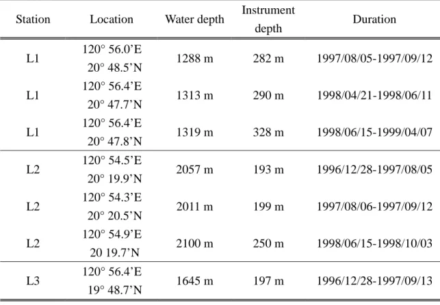
TABLE 1. Mooring locations, instrument and water depths, and durations at L1, L2, and L3, respectively.
TABLE 1. Mooring locations, instrument and water depths, and durations at L1, L2, and L3, respectively.
Station Location Water depth Instrument
depth Duration L1 120° 56.0’E 20° 48.5’N 1288 m 282 m 1997/08/05-1997/09/12 L1 120° 56.4’E 20° 47.7’N 1313 m 290 m 1998/04/21-1998/06/11 L1 120° 56.4’E 20° 47.8’N 1319 m 328 m 1998/06/15-1999/04/07 L2 120° 54.5’E 20° 19.9’N 2057 m 193 m 1996/12/28-1997/08/05 L2 120° 54.3’E 20° 20.5’N 2011 m 199 m 1997/08/06-1997/09/12 L2 120° 54.9’E 20 19.7’N 2100 m 250 m 1998/06/15-1998/10/03 L3 120° 56.4’E 19° 48.7’N 1645 m 197 m 1996/12/28-1997/09/13
Figure Captions
Fig. 1. Locations of ADCP moorings (solid circle) and wind record station (asterisk)
used in this study. The bathymetry is color shaded. It is overlaid on the
composite Sb-ADCP current velocity vectors at 30 m from Liang et al.
(2002). The reference vector is 100 cm s-1. Regions A and B show the area
of average used in Fig. 15.
Fig. 2. Time series of current velocity observed at L1. (a) U (dashed line), V
(thick solid line) components and stick diagram (thin solid vector) of the
depth-averaged (from 30 to 220 m) current velocity are shown. Vertical
sections of (b) U and (c) V components of current velocity are shown in the
middle and bottom panels, respectively. Contour interval is 50 cm s-1.
The time series was low-pass filtered to remove the fluctuations, for
frequencies higher than 0.0139 cph.
Fig. 3. Same as Fig. 2 except at L2. The range of depth average is from 20 m to
120 m in 1997 and from 140 m to 240m in 1998.
Fig. 4. Same as Fig. 2 except at L3. The range of depth average is from 20 m to
160 m.
Fig. 5. T-S diagram at L1, L2, L3, the South China Sea, and the upstream Kuroshio:
Sea, and thick line: Kuroshio. The inset shows the locations.
Fig. 6. Northeast-southwest component wind velocity (thick line) at Lanyu Island
is shown. The depth-averaged current velocity (same as Fig. 3a) at L2 is
also shown. A 5-day convolution average was applied to both wind and
current velocity.
Fig. 7. Domain of MICOM model used in this study. The land is shaded as black.
The minimum depth of ocean is 50 m. Open ocean boundary includes
about 4° sponge area.
Fig. 8. Comparisons between the monthly average velocity vectors of the
observation (thick vector) and model result (thin vector) at (a) L1, (b) L2,
and (c) L3 are shown.
Fig. 9. Comparisons between the depth-averaged current velocity of the
observation and model result at (a) L1, (b) L2, and (c) L3 are shown. The
thin and dotted lines are the U and V component of observed
depth-averaged current velocity, respectively. The thick and dashed lines
are the U and V component of model result, respectively. The ranges of
depth average are the same as Fig. 2a, 3a, and 4a, except that a 5-day
convolution average was applied to both observation and model results.
area) on 15th of (a) June and (b) December from the 10th spin up model
results are shown.
Fig. 11. Same as Fig. 10 except for the results of the model started from the 10th
spin up model results and continually forced by the 1997-2001 monthly
mean momentum flux. Current velocities at depth 50m and SSHs in
1997-2001 are shown in (a)-(e), respectively. From top to bottom, it is
shown for the 15th of March, June, September, and December.
Fig. 12. (a) Depth-averaged U in the upper 300 m water column, (b) SSH of model
results along 120.75°E from 18.5°N to 22°N are shown. A 5-day convolution average was applied to both. Shaded areas show the positive
value. Contour intervals are 10 cm s-1 and 5 cm in (a) and (b), respectively.
The 3 straight lines indicate mooring locations.
Fig. 13. Zonal volume transport along 127.5°E of model results in the upper 300 m water column between 18.5°N and 22°N is shown. A 5-day convolution average was applied. Negative and positive values represent the westward
and eastward transport, respectively.
Fig. 14. Time series of (a) northeast-southwest component of ECMWF wind stress
at L2 and (b) zonal Ekman volume transport along 120.75°E between 18.5°N and 22°N. A 30-day convolution average was applied to all.
Fig. 15. Time series of (a) SSH at A , (b) SSH at B, (c) the SSH difference between
A and B. Both the model result (solid line) and the T/P data (dashed line)
have been demeaned. A 5-day convolution average was applied to all.
The locations of A and B are show in Fig. 1.
Fig. 16. Meridional volume transports in the upper 300 m water column (a) along
18.5°N from 122°E to 125°E and (b) along 22.5°N from 15°N to 18°N of model results are shown. A 5-day convolution average was applied to
Fig. 1. Locations of ADCP moorings (solid circle) and wind record station (asterisk) used in this study. The bathymetry is color shaded. It is overlaid on the composite Sb-ADCP current velocity vectors at 30 m from Liang et al. (2002). The reference vector is 100 cm s-1. Regions A and B show the area of average used in Fig. 15.
F ig . 2. T ime series o f cu rrent v e locit y observed at L 1. (a) U (dash ed l in e), V (thick
solid line) com
pone
nts
and stick diag
ram (thin solid vector) of the dept h-aver aged (from 30 t o 220 m ) current velo ci ty are shown. V ert ical se ctions of (b) U and (c ) V com ponents of c u rrent v elocity are shown in th e middle and bottom p anels, respectiv ely . Contour inte rval is 50 c m s -1 . The t im e seri es was lo w-p ass filtered to rem ove th e flu ctuat ions, fo r fr equen ci es higher tha n 0.0139 cph .
F ig . 3. Same as Fig. 2 exc ept at L2. The range of d ept h aver age is from 20 m t o 1 20 m in 1997 and fro m 140 m to 240m in 1998.
F ig . 4. Same as Fig. 2 except at L3. The rang e of d epth averag e is f rom 20 m to 16 0 m.
Fig. 6. Northeast-southwest component wind velocity (thick line) at Lanyu Island is shown. The depth-averaged current velocity (same as Fig. 3a) at L2 is also shown. A 5-day convolution average was applied to both wind and current velocity.
Fig. 7. Domain of MICOM model used in this study. The land is shaded as black. The minimum depth of ocean is 50 m. Open ocean boundary includes about 4° sponge area.
Fig. 8. Comparisons between the monthly average velocity vectors of the observation (thick vector) and model result (thin vector) at (a) L1, (b) L2, and (c) L3 are shown.
Fig. 9. Comparisons between the depth-averaged current velocity of the observation and model result at (a) L1, (b) L2, and (c) L3 are shown. The thin and dotted lines are the U and V component of observed depth-averaged current velocity, respectively. The thick and dashed lines are the U and V component of model result, respectively. The ranges of depth average are the same as Fig. 2a, 3a, and 4a, except that a 5-day convolution average was applied to both observation and model results.
Fig. 10. Current velocity (vector stick) at 50 m and sea surface height (color filled area) on 15th of (a) June and (b) December from the 10th spin up model results are shown.
F ig . 1 1 . Sa me a s Fig. 10 e x ce p t f o r t h e r esults of the mo de l sta rte d fr o m the 10th s p in up mode l r esults a n d continually fo rced by the 1997 -2001 monthly mean mo mentum flux. Curren t velocities at de pth 5 0 m and SSHs in 1997-2001 are s hown in (a) -(e ), res p ectivel y. From top to bo ttom, it is show n for the 15t h of March , June, S ep tem b er , and D ecem ber .
Fig. 12. (a) Depth-averaged U in the upper 300 m water column, (b) SSH of model results along 120.75°E from 18.5°N to 22°N are shown. A 5-day convolution average was applied to both. Shaded areas show the positive value. Contour intervals are 10 cm s-1 and 5 cm in (a) and (b), respectively. The 3 straight lines indicate mooring locations.
Fig. 13. Zonal volume transport along 127.5°E of model results in the upper 300
m water column between 18.5°N and 22°N is shown. A 5-day
convolution average was applied. Negative and positive values represent the westward and eastward transport, respectively.
Fig. 14. Time series of (a) northeast-southwest component of ECMWF wind
stress at L2 and (b) zonal Ekman volume transport along 120.75°E
between 18.5°N and 22°N. A 30-day convolution average was applied to all.
Intra-seasonal variation in the velocity field of the
northeastern South China Sea
Chau-Ron Wu1, T. Y. Tang2,*, S. F. Lin2,3, Y. J. Yang4, and W.-D. Liang4
1
Department of Earth Sciences, National Taiwan Normal University, Taipei, Taiwan,
ROC
2
Institute of Oceanography, National Taiwan University, Taipei, Taiwan, ROC
3
Energy & Resources Laboratories, Industrial Technology Research Institute, Hsinchu,
Taiwan, ROC
4
Department of Marine Science, Chinese Naval Academy, Kaohsiung, Taiwan, ROC
*
Corresponding author. Institute of Oceanography, National Taiwan University, P.O.
Box 23-13, Taipei, 106, Taiwan, ROC, Tel: +886-2-23626097; Fax:
+886-2-23698526; Email address: [email protected]
Submitted to
Geophysical Research Letters
Abstract
Two subsurface ADCPs were deployed at the northeastern South China Sea to study
circulation structure in the area and path of Kuroshio intrusion. The 48-hour low-pass
filtered data reveal significant intra-seasonal variations in the velocity field. The
current alternates between clockwise and counterclockwise even within a single
month. Local wind stress forcing fails to address the phenomena and variations. The
present study suggests wind stress curl forcing is the dominant process controlling the
circulation picture. While a stronger curl developed off southern tip of Taiwan, it will
provide negative vorticity to the intruded current and form an anticyclonic eddy. The
stronger current is always going along with the stronger curl. On the other hand, while
the curl looses or decays, the intruded current becomes weakened and forms a
cyclonic eddy. The agreement between curl and velocity suggests that changes in the
curl contribute to the intra-seasonal variations in the region.
Introduction
The circulation structure in the northeastern South China Sea (SCS) is extremely
complicated. In addition to the location with a complicated topography and seasonal
reversal monsoon, the regions might be interacted between currents from both
might reach the sea southwest of Taiwan and influence the shelf break circulation
[Fan and Yu, 1981]. All of these factors induce varieties of contributions and alter the
current structures in the regions. Especially the intrusion current from Kuroshio front,
it might be the most important component and be the major theme in the area.
The Pacific western boundary current, the Kuroshio, flows northward and
bypasses east of Luzon and Taiwan. Similar to the Loop Current in the Gulf of
Mexico, the Kuroshio water has also been reported to intrude the Luzon Strait where
plays a deep gap in the western boundary. Seasonal variations of Kuroshio intrusion
have been reported extensively in a wealth of existing literature [e. g. Wyrtki, 1961;
Shaw, 1991]. However, the conclusion of seasonal intrusion is challenged by several
recent observations. For example, both moored current data and ship-board Acoustic
Doppler Current Profiler (ADCP) data evidenced that the westward trend of Kuroshio
intrusion is persisted all the year round [Liang et al., 2003; Tang et al., 2003].
Furthermore, although the intrusion of waters from the Kuroshio to the
northeastern SCS has been studied for several decades, the path and process of
Kuroshio intrusion in the region remained discrepancies among oceanographers. For
example, based on hydrographic data, Wang and Chern [1987] inferred an
anticyclonic (clockwise) eddy occupied the area at the onset of the northeast monsoon.
[1989] suggested that the intrusion current was probably part of a cyclonic
(counterclockwise) circulation in the northern SCS. Anticyclonic or cyclonic
circulation is of importance to the distribution of the water masses in the region. A
correct description of circulation pattern is essential to future dynamic studies of the
intrusion process.
In this study, current and hydrographic data from two mooring stations were
examined to study the circulation pattern in the region. The direct observations in the
velocity field are capable of determining the distribution of the Kuroshio intrusion
water and inferring the path of intrusion. The results show that significant
intra-seasonal variations in the velocity field. The current pattern alternates between
clockwise and counterclockwise. Wind stress curls were also calculated from the
blended QSCAT/NCEP wind stress fields at a resolution of 0.5° x 0.5° [Milliff et al.,
1999] to examine the driving mechanism of the local current.
Mooring data
Two sets of subsurface moorings (named St. W and St. E) were deployed in the
west and east of the shelf break of the northeastern SCS, respectively. Figure 1 shows
the mooring locations and the surrounding bathymetry. Each set of mooring includes
an upward-looking, 150 kHz, self-contained ADCP mounted on a 45” diameter
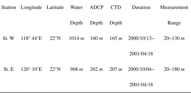
mounted 5 m beneath the ADCP. The water depths at St. W and St. E are 1014 m and
968 m, respectively. Table 1 lists the locations and local water depths for each
mooring, the depths of instruments, the duration of deployments, and the vertical
range of current profile measured by the ADCP. The bin length of ADCP was set as 8
m. The hourly current velocity was recorded averaged over 240 pings for board-band
ADCP. The standard deviations of measurement velocity were 1.2 cm s-1. The
obtained current velocity of ADCP was corrected for vertical excursion and sound
speed by the CTD data. The data were also adjusted for local magnetic deviation.
Finally, the vertical profile of current velocity was linearly interpolated and resampled
at 10 m intervals. The time series of current velocity discussed in the following
sections were low-pass filtered to remove the fluctuations for frequencies higher than
0.5 cycles per day.
Results and discussion
Low-pass filtered velocity
Figure 2 shows the eastward (U) and northward (V) components of 48-hour
low-pass filtered current velocity at St. W. Graphically, both U and V show significant
intra-seasonal variations. By November 2000, U is weak and alternates directions
between westward and eastward. The current enhances and turns eastward in
beginning of January, the eastward current decreases suddenly and reverses thereafter.
Until March 2001, a repeat behavior takes place when eastward flow appears in the
middle of March and reaches its maximum in the end of the month, turning westward
suddenly afterward. Similar pattern is presented in the V. In the end of both December
2000 and March 2001, the V turns southward after it accelerated northward.
Similar to Figure 2, Figure 3 shows U and V of low-pass filtered velocity at St. E.
Significant intra-seasonal variations are also evidenced at St. E. Graphically, U is
generally weak except in October, November 2000 and February 2001 when stronger
currents with speed more than 50 cm s-1 occur and all of them flow eastward. Two
periods of weak westward currents present in January and after middle March 2001.
Frequently reversal currents are shown in V. Prior to middle of December, currents
flow southward mostly, turning northward thereafter. Stronger southward currents
show again in the middle of February, reaching its maximum speed of 100 cm s-1 on
March 1, 2001. The current turns northward in the middle of March and persists into
April. Furthermore, the intra-seasonal variation at St. E seems to agree well with that
at St. W, indicating that St. E and St. W are related to each other somehow. To
emphasize this, the stick plots of depth average at St. W (20-130 m) and St. E (20-180
m) are shown together in Figure 4. Similar intra-seasonal reversals of currents
E generally lead those in St. W around 10~15 days. The phenomenon deserves to
further verify and will be examined in detail in the next section.
In Figure 4, northward flow prevails at St. W and southeastward flow exists at St.
E prior to the middle of December 2000. The feature infers that this region is
dominated by a conceptual clockwise circulation pattern. Currents at St. W reverse
southwestward and meanwhile currents at St. E turn either northwestward or
northeastward during the period from middle December to middle February. The
reversal phenomena suggest that current pattern alters from clockwise circulation to
counterclockwise in the study region. Clockwise circulation dominates again during
the period from middle February to middle March. Note that the currents are always
stronger during clockwise circulation. After March, weak counterclockwise
circulation plays the finale. Furthermore, as mentioned in the introduction section,
currents perform an anticyclone or a cyclone might directly influence the geographic
distribution of the water masses in the region. Without a correct description of
circulation pattern, it is not possible to identify the water masses and to verify the
intrusion process.
Water masses and circulation pattern
To describe the distribution of various water masses and the path of Kuroshio