國
立
交
通
大
學
資訊科學與工程研究所
碩
士
論
文
行 動 計 算 環 境 中 的 隱 私 權 保 護 機 制
Protecting Moving Trajectories with Dummies
研 究 生:游敦皓
指導教授:彭文志 教授
行 動 計 算 環 境 中 的 隱 私 權 保 護 機 制
Protecting Moving Trajectories with Dummies
研 究 生:游敦皓 Student:Tun-Hao You
指導教授:彭文志 Advisor:Wen-Chin Peng
國 立 交 通 大 學
資 訊 科 學 與 工 程 研 究 所
碩 士 論 文
A ThesisSubmitted to Institute of Computer Science and Engineering College of Computer Science
National Chiao Tung University in partial Fulfillment of the Requirements
for the Degree of Master
in
Computer Science
June 2007
Hsinchu, Taiwan, Republic of China
摘 要
在本篇論文中探討了利用假人的技術(Dummy-based anonymization techniques)來保護在行動環境中的使用者位置隱私權。利用製造移動方式接近 真人的假人可以保護到在行動環境中的使用者位置隱私權。然而,透過監控使用 者的長期的移動行為,他的移動路徑仍然會被暴露出來。我們認為當使用者的移 動路徑被暴露出來之後,他的位置也同時被暴露出來了。因此,為了保護用戶位 置隱私,保護使用者的移動路徑是關鍵的。我們提出了兩個製造一致的路徑的方 法,並且提出了三個測量的變數,分別是短期暴露率(short-term disclosure)、 長期暴露率(long-term disclosure)和距離差異(distance deviation)。除此之 外,我們也考慮到了使用者可能會有多條的習慣移動路徑,並提出方法加以保 護。實驗的結果證明我們所提出的方法能比目前的方法更能保護在行動環境中使 用者的位置隱私權。Abstract
Dummy-based anonymization techniques for protecting location privacy of mobile users have been proposed in the literature. By generating dummies that move in human-like trajectories, this method shows that location privacy of mobile users can be preserved. However, by monitoring long-term movement patterns of users, the trajectories of mobile users can still be exposed. We argue that, once the trajectory of a user is identified, locations of the user is exposed. Thus, it’s critical to protect the moving trajectories of mobile users in order to preserve user location privacy. We propose two schemes that generate consistent movement patterns in a long run. Guided by three parameters in user specified privacy profile, namely,
short-term disclosure, long-term disclosure and distance deviation, the proposed
schemes derive movement trajectories for dummies. Moreover, since a user may has multiple frequent trajectories, we proposed several schemes to deal with this scenario. Experimental results show that our proposed schemes are more effective than existing work in protecting moving trajectories of mobile users and their location privacy.
致 謝
兩年的碩士生涯一眨眼的時間就過了,這是一段很扎實的學習過程。要感謝 的人真的太多了,不能單單的只用『謝天』兩個字就帶過。首先要先感謝我的指 導老師 - 彭文志老師,在這兩年所給我的指導和照顧,給了我論文不少的想法 批評和指教,讓我的論文可以順利上了 IEEE 的 Workshop 以及被 invite 到 journal 去。還要感謝賓州大學的李旺謙教授,雖然人遠在國外,但是仍然不辭 辛勞幫忙改善我的論文。其次,要感謝我的口試委員陳良弼教授和黃俊龍教授, 在口試的時候提供了很多的意見,讓我可以針對本論文作更進一步的改進。除了 老師們之外,我也要感謝系辦小姐們的幫忙,適時的提醒我一些該注意的事項, 在比賽和獎學金申請的方面也幫了不少的忙,讓我的碩士生涯可以過的非常的順 利。 在實驗室中,首先要感謝學長們,無論是博班的學長 - 洪智傑,或是上一 屆的碩班學長 – 李志劭、張民憲、楊慧友和蕭向彥學長,都給了我不少在學習 和研究上的幫助,從他們那邊我學到了不少作研究的方法。其次還要感謝實驗室 的同學,鄉民、boy、佳欣大家相互鼓勵與打氣或是談論八卦的畫面我會永遠記 得。還有所有的學弟們,因為有他們的陪伴,讓我的生活充滿了歡樂。除此之外, 還要感謝一群死黨,言叡、小咪、大方、建平、大雕、P 嫂、骨感…等,你們在 我作研究苦悶的時候,給我帶來了不少的歡樂,還有平日一同去打球一起出去 玩,更讓我的研究生生涯過的十分的精彩。還有一同參與比賽的夥伴們,不管是 lab 的學長同學學弟或是我的好朋友們,真的很感謝你們,讓我的碩士班生涯過 的非常的不一樣,除了論文之外,還多出了非常多比賽的經驗。 最後要感謝我的家人,尤其是我爸媽,您們的養育之恩,以及給予我衣食無 憂的環境,讓我可以專心學習而無後顧之憂,而且常常給予我鼓勵,讓我可以更 有信心的去面對未來的挑戰。謝謝您們,永遠站在我的背後支持我,給予我莫大 的精神鼓勵,謝謝。
Contents
1 Introduction 1
2 Related works 8
3 Preliminaries 10
3.1 Assumptions and Notations . . . 10 3.2 Attacker model . . . 11
4 Generating Dummies with Patterns 17
4.1 Random Pattern Scheme . . . 17 4.2 Intersection Pattern-based Scheme . . . 18 4.3 Generating Dummies with Multiple Trajectories . . . 29
5 Performance Study 35
5.1 Simulation Model . . . 35 5.2 Experimental Results . . . 37
6 Conclusions 51
List of Tables
1.1 The real GPS log data . . . 4
3.1 An example of query log for mobile user A . . . 13
3.2 Privacy measurement of dummy trajectories. . . 14
List of Figures
1.1 Moving trajectory of one example car. . . 4
1.2 Moving trajectories of user and dummies. . . 6
3.1 Mobile behavior of mobile user A and his dummies (i.e., X and Y ) 12 3.2 Trajectories with Intersections. . . 15
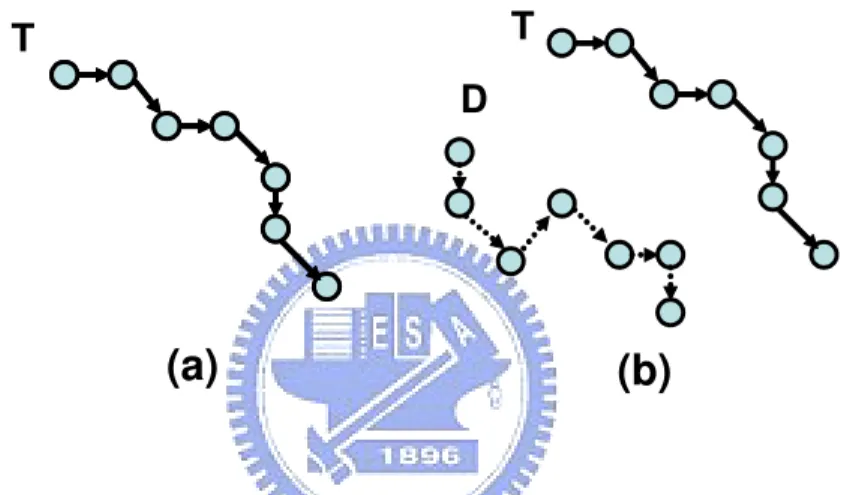
4.1 (a)original pattern (b)random pattern . . . 18
4.2 An example of executing rotate pattern scheme . . . 20
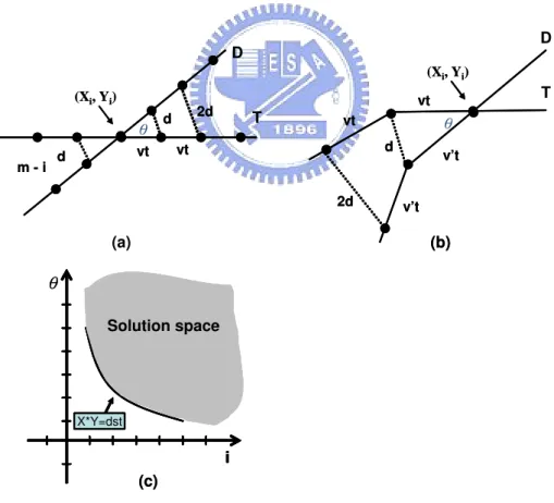
4.3 Solution space for distance derivation . . . 20
4.4 An example of the rotation pattern scheme. . . 22
4.5 Generate more intersections between dummy trajectories. . . 24
4.6 An example of 2-intersect pattern scheme . . . 26
4.7 The problem of multiple intersections . . . 26
4.8 An example of knn query caching. . . 28
4.9 An example of multiple patterns. . . 31
4.10 Two methods of select intersection point in multiple patterns. . . . 33
5.1 The needed day of exposure a user’s whole trajectory. . . 38
5.2 The performance comparison of dummy without moving patterns and dummy with moving patterns. . . 40
5.3 The performance of scheme Random, Rotate and k-intersect with LD varied. . . 41
5.4 The exposure rate of scheme Dummy, Random, Rotate and k-intersect with the number of dummies varied. . . 42
5.5 The query cost of scheme Random, Rotate and k-intersect. . . 43
5.6 The affect of query cost with the grid size . . . 44
5.7 The query cost and correct rate in different probability of multiple path(theta). . . 46
5.8 The query cost and correct rate in different probability of multiple path(data object). . . 47
5.9 The Query Cost and Correct Rate in different similarity of multiple path(theta). . . 48
Chapter 1
Introduction
Location-based services (LBSs) have emerged as one of the killer applications for mobile computing and wireless data services. These LBSs are critical to public safety, transportation, emergency response, and disaster management, while pro-viding great market values to companies and industries. Due to the unrestricted mobility of users in the mobile computing environments, users are often interested in acquiring information or services related to their current locations. Thus, very frequently locations information of users are submitted along with queries to the LBS servers. Examples of such queries include finding the nearest restaurants to a user (k nearest neighbor query) and finding ATMs within 500 meters from a user’s current location (range query). While LBSs have shown to be valuable to users’ daily life, on the other hand, they also expose extraordinary threats to user privacy. If not well protected, the location information of users may be misused by some untrustworthy service providers or stolen by hackers. Once the location informa-tion is exposed, adversaries may dig for cues to invades user privacy. Obviously, it is important to protect location privacy.
in-terests from the research community [2] [5] [15] [21] [18] [3] [16]. These studies aim at protecting exact location information of users from the potential abuse of LBS providers and hackers. Two primary approaches have been considered, including 1) trusted anonymizer based approach; and 2) client based approach. In the for-mer, users submit their queries to the LBSs via a trusted server (which is different from the LBS server), such as a base station in the cellular networks. This trusted anonymizer transforms the exact locations of a number of users into a cloaked
spa-tial area in accordance with privacy requirements set by users in order to obtain
data or services from the LBSs [10] [21] [11]. The second approach assumes no trusted server. Thus, clients are responsible for anonymizing their own location information before transmitting queries to the LBS servers. By issuing several fake locations along with its true location to the LBSs, clients may obtain redundant information or services corresponding to the submitted locations while preserving their location information [18] [19]. Unwanted information is filtered locally to ob-tain the final query results. In both approaches, the true location of a user is either 1) not distinguishable from other users (the trusted anonymizer based approach), or 2) not distinguishable from the fake locations (the client based approach). Since a trusted server is not always available, in this paper, we tackle some issues faced in the client based approach.
Motivation and Problems. Without relying on a trusted server, generating fake user locations (called dummies1) for location-dependent queries has been shown to be an effective way to preserve location privacy [18]. In addition to generate dummies based on the user locations, these prior works propose to generate
dum-1We follow the terminology used in [18] to name the fake user locations as dummy locations
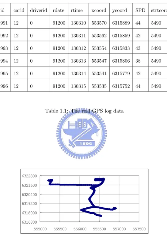
mies based on realistic user movements. However, prior works don’t consider a well-recognized observation, i.e., moving behaviors of users usually follow certain patterns [22] [23]. To demonstrate user moving patterns of users, Table 1.1 shows an example of real log data from INFATI [17]. INFATI is the first Intelligent Speed Adaptation development project in Denmark. The project is carried out by Aal-borg University. In this project, every car was equipped with a Global Positioning System(GPS) and collects day to day movements of 20 private cars on the road network of Aalborg during two months. The log data contains several attributes, such as car’s id, driver’s id(one car may be driven by more than one person), data and time, XY coordinate received from GPS receiver, speed and street code. Figure 1.1 shows one car’s trajectories, where the XY coordinate are the position coor-dinates received from GPS receiver. By exploring data mining techniques such as spatial-temporal sequential pattern mining [4] or moving pattern mining [22] [23], adversaries only need to collect enough user’s moving logs and can get the frequent moving patterns of user easily. Notice that once trajectories of users are disclosed, adversaries are able to utilize external databases to find even user identity, which incurs more serious disclose of location privacy. The above scenario is referred to the linking attack problem in location privacy, showing the justification of protect-ing user trajectories. Thus, generatprotect-ing dummies should consider not only realistic user movements but also follow certain patterns.
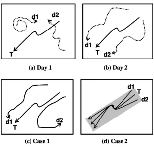
The problem we study in this paper could be best understood by an example shown in Figure 1.2. In the figure, the solid line denotes the moving trajectory of a true user (denoted as T ) and the dotted lines are generated trajectories of dummies (denoted as d1 and d2). Since true users usually exhibit certain human moving behavior, one is able to identify the solid line as a true user based on the
id carid driverid rdate rtime xcoord ycoord SPD strtcord 991 12 0 91200 130310 553570 6315889 44 5490 992 12 0 91200 130311 553562 6315859 42 5490 993 12 0 91200 130312 553554 6315833 43 5490 994 12 0 91200 130313 553547 6315806 38 5490 995 12 0 91200 130314 553541 6315779 42 5490 996 12 0 91200 130315 553535 6315752 44 5490
Table 1.1: The real GPS log data
6316800 6318000 6319200 6320400 6321600 6322800 555000 555500 556000 556500 557000 557500
typical moving behavior of humans (as shown in Fig. 1.2(a)). Thus, it’s impor-tant to generate dummy trajectories based on human moving behavior (as shown in Fig. 1.2(b)). Even though this effort may reduce the chance of the true mov-ing trajectory bemov-ing identified, a long-term movement pattern can be collected to filter inconsistent trajectories. For example, comparing the current trajectories (in Fig. 1.2(c)) and trajectories collected in a different day (e.g., Fig. 1.2(b)), one can tell T is the true trajectory of user. Once the moving trajectory of true user is identified, locations (i.e., not only the current location but also the past loca-tions) of the user is disclosed. Thus, it’s important to generate dummies that not only demonstrate moving behavior of users but also follow consistent, long-term movement patterns.
Given that the adversaries obtain a set of trajectories, they will have difficulty determining the true trajectory of a user if users generate dummies following certain movement patterns. However, the user trajectory is still disclosed to a certain de-gree. Therefore, we use disclosure to denote the probability that the user trajectory may be correctly identified by the adversaries. For example, in Fig. 1.2(c), three trajectories are collected and thus the disclosure is 1
3. To reduce the disclosure, a naive approach is to simply increase the number of dummies, which however incurs overhead in terms of query message length and thus communication and client processing costs. Thus, in this paper, we propose to generate intersecting
dummy trajectories aiming at increasing the number of possible trajectories from
the adversaries’ perspective and thus decreasing disclosure of the user trajectory. Nevertheless, an issue exists with this intersecting trajectories. When the gen-erated trajectories are too close to the true trajectory, the locations of a user may still be exposed, e.g., Fig. 1.2(d) shows an example where the user’s moving
trajec-T d1
d2
(a) Day 1 (b) Day 2
T d1 d2 d1 T d2 (c) Case 1 (d) Case 2 T d1 d2 T d1 d2 T d1 d2
(a) Day 1 (b) Day 2
T d1 d2 d1 T d2 (c) Case 1 (d) Case 2 T d1 d2 d1 T d2 (c) Case 1 (d) Case 2 T d1 d2 T d1 d2
Figure 1.2: Moving trajectories of user and dummies.
tory (the shadowed path) can be identified. Thus, our design of dummy generation schemes also take the factor of distance deviation among trajectories into consid-eration. Our approach is to allow users to set up their privacy profile in terms of disclosures (both short-term and long-term) and distance deviation (more details to be discussed in Section 2). We propose two schemes, namely, random pattern and
intersection pattern, to generate dummy trajectories based on the privacy profile.
Furthermore, since a user may have more than one moving trajectories, we develop several schemes to protect multiple user moving trajectories with the purpose of using minimal number of dummies. Performance of proposed schemes is compara-tively analyzed and sensitivity analysis on several design parameters is conducted. Experimental results show that by generating dummies based on moving patterns, our schemes perform better than the existing techniques.
Organization. The rest of this paper is organized as follows. We first describe some related works in Section 2. Section 3 presents preliminaries, including attacker model and user profile. Our proposal of dummy trajectory generation schemes and
the selection of multiple path are presented in Section 4. Section 5 shows our performance study. Section 6 concludes this paper.
Chapter 2
Related works
A significant amount of research efforts have been elaborated on location pri-vacy. Generally speaking, methods of guaranteeing location privacy could protect either user’s identification or user’s location. Because most Location Informa-tion(LocInfo) can be a variation of the definition introduced in [8], the triple of the following form: Position, Time, ID. Thus, LocInfo is defined as a combination of the “Position” that the entity with identifier “ID” maintained at time “Time”, within a given coordinate system. Position and ID are considered as the most important part in LocInfo. Protecting identifier is to hide user’s identifier that attacker cannot take apart who is exactly in this position at this time. Different from ID, Protecting position is to protect user’s location from being disclosed that the attacker cannot recognize the user’s exactly position at this time.
Specifically, to protect ID in LocInfo, the authors in [2] [5] proposed the con-cept of the mix zone [2] [5]. They assumed the LBS application providers are hostile adversaries, and suggested that application users hide their own identifier from providers [3]. So they proposed the mix zone concept in which a trust third party removes all samples before is passes location samples to the LBS application
providers. Instead of static mix zones, the authors in [16] implemented a mix zone concept by exploring a silent period. That protects user from correlation attack which means a method of utilizing the temporal and spatial correlation between the old and new pseudonym of nodes.
To protect user location, a consider amount of research works are conducted [15] [21] [18] [19]. As described before, these works could be further classified according to the architecture of location privacy. With trusted servers, the authors in [13] [12] [11] proposed a cloaking algorithm to blur the resolution of location information along spatial and temporal dimensions. The above algorithm exploits k-anonymity concept. Based on k-anonymity, the authors in [10] [9] devised a personalized and customized k-anonymity model which assume a different k-anonymity requirement for each user. A framework Casper was developed in [21], where a grid-based pyramid structure is implemented to index all user locations. Moreover, privacy-aware query processing is developed when cloaked spatial areas are used as query predicates. Without trusted servers,the authors in [7] proposed 1 P2P structure to protect user’s privacy. Explicitly, before issuing any location-based service queries, mobile users will form a group from his/her neighboring peers via multi-hop routing. Then, the spatial cloaked area is computed as the region that covers the entire group of peers. In addition, the authors in [18] [19] proposed an algorithm to generate dummy locations to protect not only location privacy but also true user identifications.
To the best of our knowledge, prior works neither address location privacy issues from long-term observation nor emphasize the necessity of protecting user moving patterns, let alone generating dummies with moving patterns. This paper differentiates from other papers.
Chapter 3
Preliminaries
In this section, some preliminaries are given. In Section 3.1, assumptions and notations used in this paper are presented. The attacker model and user privacy profiles are described in Section 3.2.
3.1
Assumptions and Notations
We assume no trusted server available for location anonymization. Wireless net-works are only responsible for communication and will not reveal locations of mo-bile users. Momo-bile clients are location aware (via GPS or network based positioning techniques). To facilitate the presentation of our paper, suppose that users are free to move in the space divided into grid cells. Each grid cell has a cell identifier (x, y) indicating that this cell is located at the x column and the y row of the space. The granularity of this representation is determined by the number of grid cells. With larger number of grid cells, finer granularity we have. Note that using cell identi-fication could achieve a certain level of location privacy even if adversaries guess the true location among a set of location data.
Upon a user query message, the mobile client Ui first sends to the LBSs through
an authenticated and encrypted connection that adversary cannot hijack the mes-sage. A query message issued by a mobile user Ui to a LBS server at time slot
t is defined as M = {uid, hLt
i, Ltd1, Ltd2...Ltdni Q}, where uid is the pseudonym
user identification, Lt
i is the true user location, Ltd1, Ltd2, ..., Ltdn are n dummy
lo-cations, respectively, and Q is the location-dependent query issued. Therefore, given m consecutive queries, we define the trajectory of a moving client in 2-dimensional (2D) spaces as a sequence {L1
i, L2i, ..., Lmi }, while the trajectory of
dummy x is { L1
dx, L2dx, ..., Lmdx}) where Lai ∈ R2 (a = 1, ..., m) describe locations in
ta, t1 < t2 < ... < tm ∈ T are irregularly spaced but temporally ordered time
in-stances, i.e., gaps are allowed. Here, Lji (and Lm
dx, respectively) denotes the location
of user Ui (and dummy dx), respectively at the jth time slot. Denote a trajectory
of mobile user Ui as Pi = {P L1i,, P L2i, ..., P Lmi }, where P Lji is the location of mobile
user Ui at the jth time slot. Suppose that the length of trajectories is m and the
maximum user’s moving velocity is defined as Vmax.
3.2
Attacker model
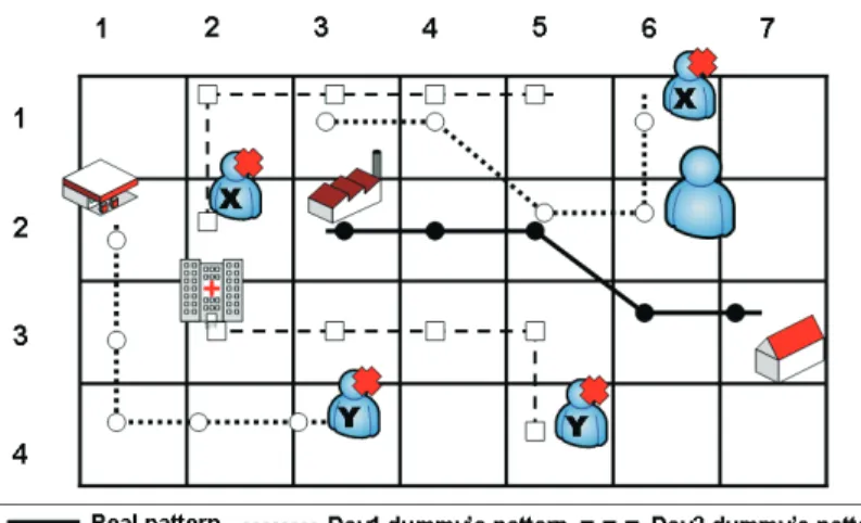
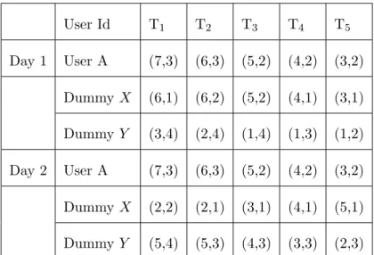
In this section, we describe how adversaries collect and utilize data mining tech-niques to mine user moving patterns. Explicitly, adversaries can sequential pat-tern mining to discover user moving patpat-terns, thereby disclosing user trajecto-ries. [1] [14] [4]. Consider an example shown in Figure 3.1, where Table 3.1 is the moving log. As can be seen in Table 3.1, there are five movement sequences, where each location in a movement sequence is the cell identification defined in Section 3.1. Given the minimum support 2, it can be verified that a moving pattern (i.e.,
Figure 3.1: Mobile behavior of mobile user A and his dummies (i.e., X and Y ) (7,3)⇒(6,3)⇒(5,2)⇒(4,2)⇒(3,2)) is discovered.
Once moving patterns are discovered, one could easilyidentify true user posi-tions, no matter how dummies are generated. The main theme of this paper is to prevent a privacy threat resulting in long term movement observations. Three formal definitions of privacy preservation are given as follows:
Definition 1. Given an area size A ∈ R+, a mobile user’s trajectory P
i and
n dummies, the probability of successfully identifying the true user’s trajectory is
smaller than the profile user define.
Definition 2. Given an area size A ∈ R+, a mobile user’s current location L and n dummies, the probability of successfully identifying the true user’s current location is smaller than the profile user define.
Definition 3. Given an area size A ∈ R+, a mobile user’s trajectory P
i and n
dummies, the average distance difference among trajectories of dummies and the user must be larger than the profile user define.
By these definitions, an adversary cannot distinguish user’s trajectory or loca-tions. As such, both location and trajectory privacy can be preserved. Users may
User Id T1 T2 T3 T4 T5 Day 1 User A (7,3) (6,3) (5,2) (4,2) (3,2) Dummy X (6,1) (6,2) (5,2) (4,1) (3,1) Dummy Y (3,4) (2,4) (1,4) (1,3) (1,2) Day 2 User A (7,3) (6,3) (5,2) (4,2) (3,2) Dummy X (2,2) (2,1) (3,1) (4,1) (5,1) Dummy Y (5,4) (5,3) (4,3) (3,3) (2,3)
Table 3.1: An example of query log for mobile user A
set up their privacy profile, which is specified by the following three parameters: 1. Short-term Disclosure (SD): This parameter specifies requirement for
protecting the current user location. Thus, given a set of current locations (including true and dummy locations), SD is the probability of successfully identifying the true user location, i.e., SD = 1
m
Pm
i=1|D1i|, where m is the number of time slots in a trajectory, Diis the set of true and dummy locations
at the ith time slot, and |Di| is the size of Di.
2. Long-term Disclosure (LD): This parameter specifies requirement for pro-tecting the user trajectory. Given n trajectories, among which k trajectories have intersected with other trajectories and (n − k) trajectories do not have any intersection. Thus, for those (n − k) trajectories, we have exactly (n − k) possible trajectories. For those k trajectories, we may enumerate all possible trajectories by exhaustively traversing intersections from the start point of each trajectory to the end point. In order not to distract readers from the main theme of this paper, we simply denote the number of possible
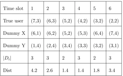
trajecto-Time slot 1 2 3 4 5 6 True user (7,3) (6,3) (5,2) (4,2) (3,2) (2,2) Dummy X (6,1) (6,2) (5,2) (5,3) (6,4) (7,4) Dummy Y (1,4) (2,4) (3,4) (3,3) (3,2) (3,1) |Di| 3 3 2 3 2 3 Dist 4.2 2.6 1.4 1.4 1.8 3.4
Table 3.2: Privacy measurement of dummy trajectories.
ries by BFS(Breadth-First-Search) among k trajectories as Tk. Consequently,
we have LD as 1
Tk+(n−k).
3. Distance deviation: The distance deviation (dst) is the average of distance difference among trajectories of dummies and the user. As a result, dst of mobile user Ui is formulated as m1 ∗1n∗
Pn
k=1
Pm
j=1dist(P Lji, Ljdk), where dist
is distance between the true user location and dummy locations in unit of cell size.
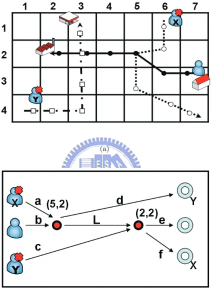
Figure 3.2 shows an example of generated dummy trajectories with intersec-tions, while Table 3.2 shows the trajectories as well as the number of current locations (Di) and distance deviation at different time slots. Thus, we can
de-rive SD = 1 6( 1 3 + 1 3 + 1 2 + 1 3 + 1 2 + 1 3) = 7
18. Furthermore, for each time slot, we could derive distance differences between dummy and true trajectories to obtain the average distance deviation as 2.47. To facilitate the derivation of total possible trajectories, Figure 3.2(a) is transformed into Figure 3.2(b), where intersection points (i.e., cell (5, 2) and (3, 2)) are marked. Since these three trajectories have two intersection points, it can be verified that we have 8 possible trajectories (i.e.,
(a)
(b)
ad, aLe, aLf, bd, bLe, bLf, ce, cf). As such, we could have long-term disclosure
LD = 1
Chapter 4
Generating Dummies with
Patterns
Given a privacy profile, our goal is to generate dummy trajectories that satisfy the user-define parameters in privacy profile (SD, LD, dst). In this section, we propose several schemes, namely, random pattern scheme and intersection pattern-based
schemes to generate dummies that exhibit long-term user movement patterns.
4.1
Random Pattern Scheme
In this scheme, the starting point and the destination of a dummy are first selected. Then, the grid cells between the starting point and the destination are determined based on the speed of a dummy and four movement types, including horizontal movement, vertical movement, both and stay in the current position. Because the humans moving speed is limited, the velocity of dummies should also be limited (i.e. smaller than Vmax). Figure 4.1(b) is an easy example with random dummy
In this scheme, a dummy will move randomly from the starting point towards the destination. This naive scheme demonstrates that even after a long term obser-vation, it’s difficult for adversaries to identify true user since dummies also exhibits long term, consistent movement patterns. Given the original user moving trajec-tory in Figure 4.1(a). Figure 4.1 shows a dummy trajectrajec-tory generated by random
pattern scheme. However, without taking into account factors such as distance
de-viation, this scheme simply include more dummies when the privacy requirements are not satisfied.
(a)
(b)
T
T
D
Figure 4.1: (a)original pattern (b)random pattern
4.2
Intersection Pattern-based Scheme
The main idea in this scheme is to have some intersections between trajectories of dummies and the real user that can generate more possible trajectories. Adversaries are harder to identify a true user trajectory from a set of possible trajectories. The benefits of using intersection pattern scheme are described below. First, if the num-ber of intersections among a user trajectory dummy and trajectories are increased, one can use smaller number of dummies to satisfy the LD in user profile. Second, it is hard for adversaries to tell which trajectories are made by dummies. Third, if
dummies have some intersections with true user by using caching technique, data requested by dummies are used by a true user in his future movement.
In this intersection pattern scheme, generated dummy trajectories should ful-fil the privacy proful-file of the user. Since there are three requirements in privacy profiles, our approach is to first select intersections from the candidate set. The candidate set depends on some constraints(i.e., important place, query cost) which we will discuss later. Afterward, our approach derive the solution space for the requirement of distance derivation. Then, within this solution space, we obtain the short-term and long-term disclosures (i.e., SD and LD). The trajectories with disclosures smaller than what specified are selected as dummy trajectories. With proper selection of dummy trajectories, we can minimize the number of dummies so as to satisfy the user privacy requirements. In view of the concept we mentioned above, we proposed two kinds of intersection dummy generation: rotation dummy
generation and k-intersect dummy generation.
4.2.1
Rotation Dummy Generation
Given a user trajectory, we generate a new trajectory for a dummy by rotating the known user trajectory in the rotation pattern scheme. To perform a rotation on a user’s sequential pattern, the rotating point and the rotating angle must be decided. Clearly, the rotation point of user trajectory is an intersection point. Consider Figure 4.2 as an example, where the dotted point is the rotate point and
θ is the rotate angle.
In order to derive the solution space for the distance derivation (i.e., dst), both the rotation angle and the rotation point within a true user trajectory have a great impact on the distance deviation. To simplify the derivation of distance deviation,
Ӱ
T
D
Ӱ
T
D
Figure 4.2: An example of executing rotate pattern scheme
(b) Ӱ (Xi, Yi) d 2d vt vt v’t v’t (b) Ӱ (Xi, Yi) d 2d vt vt v’t v’t i Ӱ Solution space X*Y=dst (c) i Ӱ Solution space X*Y=dst i Ӱ i Ӱ Solution space X*Y=dst (c) (a) Ӱ d (Xi, Yi) vt m - i 2d d vt Ӱ d (Xi, Yi) vt m - i 2d d vt T D T D
assume that we have a true user trajectory in Figure 4.3(a), we assume the real user’s moving speed is v and the distance between two consecutive movements can be represented as vt. The rotation point is the location at the ith time slot in a true user trajectory, denoted as (Xi, Yi), and the rotation angle is θ. d is the distance
difference between the location of a true user and that of a dummy at the (i + 1)th time slot. According to the cosine theorem, we have d =√2|vt|√1 − cos θ. Hence, we could derive that the distance deviation of these two trajectories as follows:
dstr = 1 m ∗ ((d + ... + id) + (d + ... + (m − i)d)) = √2|vt|√1 − cos θ ∗ ( i X j=0 j + m−i X j=0 j)
If user trajectories are not straight lines, the above derivation is still held. Consider two realistic trajectories in Figure 4.3(b). In order to make the distance of two corresponding points at (i + 1)th time slot be d, we could dynamically set up the dummy’s speed to v0(0 5 v0 5 V
max). The distance of the following points
along these two trajectories is the multiple of d. Similarly, we can get the following formulas:
d =p(vt)2+ (v0t)2− 2vv0t2cos θ
Because v and v0 are also constant, we can derive to the following formula.
dstr =pC 1− C2cos θ ∗ ( i X j=0 j + m−i X j=0
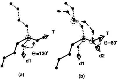
Ә=120̓ T d1 T d1 d2 Ә=80̓ (a) (b) Ә=120̓ T d1 T d1 d2 Ә=80̓ (a) (b)
Figure 4.4: An example of the rotation pattern scheme.
From the above derivation, we could conclude that both the rotation angle (i.e.,
θ) and the rotation point (i.e., i) have an impact on the distance deviation.
As-sume that we have n dummies trajectories and the distance deviation of n dummy trajectories is dstn. If one dummy is added into the set of n dummies, the (n + 1)
dummies should be larger or equal to the requirement of distance deviation (i.e.,
dst). Thus, we have the following formula: n
n + 1dstn+
1
n + 1dst
r ≥ dst
Consequently, when one dummy is added into the current set of dummies, this dummy should have a constraint on dstr ≥ (n + 1)dst − n(dst
n). Therefore, we
could have a solution space shown in Figure 4.3(c). For each point (expressed by (θ, i)) in the solution space, we should calculate the corresponding disclosure. Hence, a solution point with the minimal hit probabilities is selected. If the hit probabilities are still larger than the required hit probabilities, one should repeat the above procedure to add one additional dummy until the all privacy criteria are satisfied.
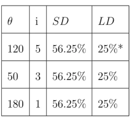
For example, consider a true trajectory (the line marked with T) in Figure 4.4(a) and a user privacy profile (i.e., SD = 40%, LD = 10%, dst = 2.1). Initially, there is no dummy (i.e., n = 0) and dst0 = 0. As such, we could have dstr ≥ (0 + 1) ∗ 2.1. Table 4.1(a) show some selected possible solution space when the number of dummy is 0. In Table 4.1(a), the solution (i.e., (120o, 5)) is selected and then n is increased to 1. The value of dst1 is updated accordingly. However, since disclosures are still larger than the required values (i.e., 56.25% ≥ 40% and 25% ≥ 10%), we should add one more dummy to reduce the disclosures. Following the same procedure, we have dstr≥ (1 + 1) ∗ 2.1 − 1 ∗ 2.8 and Table 4.1(b) is the solution space when the
number of dummy is one. From Table 4.1(b), one could select (80o, 6) since the corresponding disclosures is smaller than the required values and it needn’t to add one more dummy. Hence, Figure 4.4(b) shows the final dummy trajectories.
If we can generate more intersections between each trajectory1, we can use less dummies to generate more possible trajectories for lower disclosures. Assume we add one dummy d2 in Figure 4.5, dummy d2 has intersecttions with real user T and dummy d1. The intersection of trajectory i and j denotes as Ii,j. We can
indicate the distance between IT,d1 and Id1,d2 is L, and the distance between IT,d2
and Id1,d2 is D in Figure 4.5. Assume the rotation angle between T and d1 is α
and rotation angle between T and d2 is β, we want to find the suitable rotation point and rotation angle that can make d2 intersect with d1 and T . We use sine theorem in Figure 4.5.
D
sin(β − α) =
L
sin(180◦− β)
Then we can derive the following formula.
θ i SD LD
120 5 56.25% 25%*
50 3 56.25% 25%
180 1 56.25% 25% (a). Solution space when n=0
θ i SD LD
170 8 37.5% 16.67% 120 7 37.5% 12.5%
80 6 39.6% 8.33%*
(b). Solution space when n=1
Table 4.1: A solution space.
Θ β Θ β α Θ α Θ β Θ β α Θ α
If β ≥ α m − i D ≥ L D = sin(180◦− β) sin(β − α) = sin β sin(β − α) If β < α m − i D ≥ L D = sin(180◦− α) sin(α − β) = sin α sin(α − β)
From the above derivation, we could reduce the candidate sets of rotation point
i and rotation angle β because i and β must satisfy the formula to make another
intersection. Consequentially, the solution space is further reduces. Based on achieving user’s all requirements, when adding one dummy each time, we intend to generate more intersections to reduce the total number of dummies.
4.2.2
K-intersect Dummy Generation
Rotation dummy generation only has one intersection between user’s trajectory and dummies. If the number of intersections between a user and the dummies are increased, it is more difficult for adversaries to figure out the user’s true trajectory and LD is thus decreased. But the dst is also influence a lot. Besides, in the situation that attackers has some background knowledge of users, the intersections between a user and the dummies can decrease the exposure of users’ trajectory and thus protect users’ location privacy. In this scheme, we increase the number of intersections between user trajectory and the dummy trajectories.
This scheme selects k points from the intersection candidate set to be the inter-section points. Then the paths between the interinter-section points by the randomized dummy generation. The intersection points can be represented as C = C1, C2, ..., Ck
intersec-Ӱ Ӱ Ӱ Ӱ T D
Figure 4.6: An example of 2-intersect pattern scheme
Figure 4.7: The problem of multiple intersections
tion points, the rotation dummy generation is used. Explicitly, C1 and Ck can be
regards as the rotation points and the following formula is used:
(m − k) ∗ dstr+ k ∗ dstk
m = dst
=⇒ dstr =
m ∗ dst − dstk∗ k
m − k
dstk means the distance deviation and a means the length of trajectory between
the cutting points C1 and Ck. The combinations of the paths describe above
will be outputted as the dummy’s moving pattern. An example of 2-intersect dummy generation example is shown in Figure 4.6, where the dotted circles are the intersection points. The trajectory in dotted square is generated by randomized dummy approach and beyond the square is generated by rotation dummy approach. Note that increasing the number of intersection points is not always good. Be-cause the more intersections between user’s and dummy’s trajectories the less dis-tance derivation the user has. For example, in Figure 4.7, the dummy’s trajectory
is too closed to user trajectory. That will cause the injury of dst and attacker may break user’s privacy level. In this paper, we set the value of k is two to make more intersection than the rotation dummy generation and not hurt the quality of privacy in value dst.
As mentioned before, the selection of intersection candidate sets depends on several factors. We explore two factors to select candidate sets. First, the candidate sets should not be an important place to the user. For example, if we choose a users home as the intersection point, dummies and the user will stay in the same cell for a long period of time. Therefore the dummy cannot effectively protect the users location privacy. Second, in order to increase the cache utilization, we develop a cache scheme to determine intersection points in which users are likely to visit.
To determine which places are important, we should consider the staying time and sensitive places. Obviously, choosing a place that the user stays for a long time as the intersection point will decrease the location anonymity. The other type of important place is sensitive area [6], sensitive area means the places(e.g., hospital, nightclub) user don’t want people know that he is inside. For example, when shopping in a mall, most people may not be very concerned even if their locations are known. However, users may worry about their locations exposed (e,g, hospital). Our method will exclude those important places, which including the place that user stayed for more than threshold slots Tmax and user-specific sensitive
area Si, to form the remainder for candidate position set.
In dummy techniques, communication cost increases are generated as a side effect. Since, the service provider must create a reply message not only for the true position data but also for the dummy. In dummy methods, LBSs will return both users’ and dummies’ data, user will filter out the dummies requests. That
Figure 4.8: An example of knn query caching.
is undoubtedly a waste of resource. Caching dummy data for future use is possi-ble, if select intersection points before that a user is likely to stay. Not only the intersection but also the area near the intersection could be cached. Adding a dummy trajectory intersects user’s trajectory at different time slots in the gener-ating dummy scheme. Consider Figure 4.8 as an example, where KNN queries are issued. Initially, we retrieve more than k data sources and let dummy X arrive the intersection (2,5) before the arrival of this user. Thus, the data returned for dummy X when X is used to arrive at intersection (2,5).
Based on the above concept, we employ query cost to evaluate the performance. The query cost QCd is defined as:
QCd= (n + 1) ∗ m X i=1 SZi− ((n + 1)Ibt+ If t+ Iat) ∗ k X j=1 SZj
The first term represents the query cost of dummy method. SZi and SZj mean
the size of answer messages, n and m mean the total number of dummies and the total time slot respectively. The second term represents the saved query cost of
cache. Ibt are the intersection points before the user arrive, Iat are the intersection
points which dummy and user arrive at the same time and If t are the intersection
points after the user arrive. Because Ibt are beneficial for the cache scheme, user
and dummy needn’t query when user arrive the Ibt. If we want to lower the query
cost, one should increase the number of Ibt.
Dummies should arrive to the P Li early, we can derive that P Lt1d = P Lt2 and
t1 < t2, where P Lt1
d is the dummy’s location at time slot t1 and P Lt2 is the user’s
location at time slot t2. Figure 4.8 shows an example of query cost, dummy X arrives the position (2,5) before user and there are two dummies and five time slots. Assume that the size of answer messages(SZ) are 10, it can be verified that
QCd=(2 + 1) ∗ 50 − (3 ∗ 1 + 0 + 1) ∗ 20 = 70 in this example.
4.3
Generating Dummies with Multiple
Trajec-tories
According to the research in [23], a user in general has multiple moving trajec-tories. Consider Figure 4.9(a) as an example, where a userhas four frequent tra-jectories and each has different probabilities. This user goes to his office with
A%, B% to the hospital, to the gas station with C% and the park with D%.
Every person has different static frequent trajectories and each trajectories has distinct probability. Our method should also guarantee the user profile if user is on his frequent trajectories. Each user has k moving trajectories with cor-responding with probabilities p1, p2, ...pk and these trajectories are denoted as
{(P L1
i(p1), P L1i(p2),. . . , P L1i(pk)), (P L2i(p1), P L2i(p2),. . . , P L2i(pk)),. . . ,(P Lmi (p1),
P Lm(p
jth time slot with the probability pk. Notice that
Pk
i=1pimay not be 100% because
we only consider about frequent trajectories. Trajectories with smaller probabil-ities are not considered. We propose two schemes, namely, Multiple Path
Selec-tion(MP S) and Multiple Path without SelecSelec-tion(MP wS). In the MP S scheme,
we also present two types of dummy generation, named Multiple Random Dummy
Generation(MRANDG) and Multiple Rotation Dummy Generation(MROT DG).
4.3.1
Multiple Path without Selection (MP wS)
Given user trajectories with probability p1, p2, ...pkand user profile, scheme MP wS
generates dummy trajectories for each trajectory. Suppose that each trajectories will generate n dummies, we will have k ∗ n dummy trajectories, where n is the number of dummies.
Although this method certainly guarantees for each trajectories for the privacy profile, the number of dummies is huge. As a result, the query cost will increase as well. Therefore, we proposed Multiple Path with Selection(MP S) that consider the probabilities of trajectories for dummy generation of each trajectories.
4.3.2
Multiple Random Dummy Generation (MRAN DG)
In multiple random dummy method(MRANDG), each dummy creates k dummy patterns with probability p1, p2, ...pk, which is the same as user’s trajectories. So it
should generate k ∗ n dummy trajectories, where n is the number of dummies se-lects dummy trajectories with each probability. Take Figure 4.9 for an illustration, Figure 4.9(a) shows the original user’s four trajectories with different probabil-ity(A%, B%, C%, D%) respectively. Using the random dummy algorithm to add one dummy in Figure 4.9(b), it is obviously to see that dummy X generates four
dummy trajectories with the probability A%, B%, C%, D% respectively. Note that the privacy profile is not guaranteed, since the selection of dummy patterns is accordance with the probabilities. The other problem is user people’s trajectories usually have partial similarity in that user’s moving trajectories are also have some common sub-trajectories [20] [4]. In Figure 4.9(a), user’s moving trajectories are also have some common sub-trajectories, but the dummy X’s trajectories have no similar portions of the trajectories.
4.3.3
Multiple Rotation Dummy Generation (MROT DG)
Considering about that patterns usually has partial similarity, it is defined δ to measure the similarity of dummy trajectories and user trajectory. If δ = 0%, these two trajectories don’t have any overlap, if δ = 100%, these two patterns are totally the same. Let B denote a user moving behavior set that we can represent B(Ui) =
δ1, δ2, ..., δk where δi means the similarity of trajectory i with probability pi. All
the moving behavior δi are compare to the most frequent trajectory. Considering
in rotation dummy generation, we try to make all the trajectories satisfy user’s profile. Our key idea is that we rotate the whole trajectories with the same angle
θ at the rotation point i to solve the selection problem. If a user is on the branch
point, dummy will be able to select the suitable dummy trajectory. Figure 4.9(c) shows an example of selection rotation point as γ. The selection of the rotation point i and rotation angle θ are proposed as follows:
Possibility Based Method(P BM ): Each dummy will generate k different dummy trajectories with different probability. These k dummy trajectories have its own solution space. We can divide it into two situation - rotation angle selec-tion and rotaselec-tion point selecselec-tion. The key idea of this method is to find out the
100% 10% 10% 10% 90% 90% 10% 10% 20% 20% 70% 70% 100% 70% 70% 70% 30% 30% 10% 10% 20% 20% 10% 10% Probability Pattern (a) (b) 100% 10% 10% 10% 90% 90% 10% 10% 20% 20% 70% 70% 100% 70% 70% 70% 30% 30% 10% 10% 20% 20% 10% 10% Probability Pattern (a) (b)
Figure 4.10: Two methods of select intersection point in multiple patterns. most probability in the sub-trajectories. In other words, we want to find out the intersection i which can calculate the maximum of Paj=0P Li(p
j). a is the sum of
the location in each trajectory probability. Every trajectory has its own solution space about θ and i, so we can find out the overlap of rotation angles θ easily. First at all, we find out the rotation point i, which makesPaj=0P Li(p
j) maximum.
Depend on the rotation point, we find filter out some rotation angles in solution space. The remaining rotation angles are θ.
Figure 4.9 shows a multiple trajectories of a real user. The candidate of rotation point is in the whole trajectories. We sort the candidate positions in order of time and position are shown in Figure 4.10(a), which probabilities with A = 70%, B = 10%, C = 10%, D = 30%. First at all, we exclude the important place(i.e., home) and find out the highest probability to be the rotation point, in this example is the position with 90% probability. Then we use this constraint to find out the suitable rotation angle θ. This method can guarantee most quality of user’s trajectory privacy. In the method, selection will not be a problem. User and dummy will have same sub-trajectories, so dummy also has the graph like 4.10(a) and know
which trajectory should be chosen.
Trajectory Based Method (T BM ): The approach is different from the possibility based method in rotation point selection. Possibility based method is based on selection highest probability location for the intersection. Trajectory based method is based on the number of trajectories. The intersection i selects the largest number of trajectories pass through.
Assume that A = 10%, B = 10%, C = 10%, D = 70%, and we exclude the important place and find out the location which has most trajectories pass through. In Figure 4.10(b), the position with 30% probability will be chosen, not the position with 70% probability. This method will guarantee most trajectories but not highest probability.
Chapter 5
Performance Study
In this section, we evaluate the performance of our proposed schemes and conduct experiments to evaluate our dummy generation scheme. We first describe the simulation model in Section 5.1 and we will show the experimental results in Section 5.2.
5.1
Simulation Model
In our simulation, we use two kinds of trajectory sets, one is the real data - INFATI [17] data set and the other one is our trajectory generator. The INFATI data derive from the INFATI Project, which was day to day movements of several private cars on the road network of Aalborg. We select one car’s moving log for the real data set. In order to discuss conveniently. We use integer as unit time instance and set the whole time period from 0 to 50. The entire area within which the car has been moving is divided into grid of size 100*100. Because the data set is sampling every second when car drove, we assume the moving object send his request every
Our trajectory generater is divided the space into 50*50 grid cells which size is 10m*10m. Assume that the number of time slots is 20. Moreover, We sim-ply assume that there exists k moving trajectories for each user with probability
p1, p2, ...pk and partial similarity δ1, δ2, ..., δk, (i.e., the pattern has a starting point
and a destination point). Then, those grid cells between the starting point and the destination are selected based on the nature of movements, (i.e., the next move is a neighboring cell of the current location). Three movement types are implemented, the horizontal movement, the vertical movement, and both. To emphasize the pri-vacy threat of long-term observation, we implemented the prior work in [18] [19] as scheme dummy. Suppose that adversaries are able to collect the query log in which the movements of dummies and true users are recorded. Adversaries may explore data mining techniques [23] to discover movement patterns of users.
To evaluate the simulation result, performance metrics are Number of dummies,
Pattern Exposure Rate, Correct Rate and Query Cost for the evaluation.
Number of dummies:Number of dummies is the number of dummies needed to satisfy the privacy profile
Pattern Exposure Rate:Pattern Exposure Rate can be represented as the for-mula Pattern Exposure Rate= The trajectory exposed by the attacker
The total time slots of trajectory
Correct Rate:Correct Rate is that the proportion of dummy selected the right trajectory.
5.2
Experimental Results
We will discuss the settings and prove that long term observation will expose user’s trajectory and compare with the the Kido’s dummy [18] under different settings in Section 5.2.1. In Section 5.2.2, we will compare our method in several aspects the number of dummy and the saving of resource. Finally, we present the correct rate of different approaches in multiple trajectories.
5.2.1
Comparison to Dummy
We use the INFATI data set for the real data. In first experiment, we will show that how many days of query logs if the attacker collects will exposure the whole trajectory. We pick up one car which data was collected during December 2000 and January 2001 and our trajectory generator for the experiment. We control the coefficient of variation of query’s sampling. Assume that user’s query is discrete uniform distribution, then compare with different query probability is 20%, 50%, 80%, 100%. We assume the adversaries user the sequential pattern mining and the support is set to two and the confidence is set to 50%. Figure 5.1 shows the experimental results. The needed days is shown on the X-axis and the pattern
exposure rate is on the Y-axis. pattern exposure rate represents the total pattern
guessed by the adversaries. If the pattern exposure rate is closed to 100% that means the attacker has high probability to hit the real trajectory. We can see the result in Figure 5.1 that user’s moving trajectory can be exposed as long as the attacker get enough moving logs. If we assume the attacker set the minimum support 2 and the minimum confidence 50%, we can see the result in Figure 5.1(a)and(b) that the lower the query sample the more the attacker should collect. If the query sampling
0 20 40 60 80 100 1 2 3 4 5 6 7 8 9 10 Pattern Exposure(%) Number of Days 20% 50% 80% 100%
(a) Our dummy generator
0 20 40 60 80 100 1 2 3 4 5 6 7 8 9 10 Pattern Exposure(%) Number of Days 20% 50% 80% 100%
(b) INFATI data set
arrives to 100%, the attacker only need 3 days and 6 days moving logs to exposure the user’s whole trajectory in our pattern generator and INFATI data, respectively. We now investigate the impact of movement patterns. Suppose a privacy profile is set to SD = 20%, LD = 10%, and dst = 2.8. We compare our rotation pattern scheme with the dummy scheme. Figure 5.2 shows the experimental result. In Figure 5.2(a), it can be seen that when the amount of data collected increases with the time, both SD and LD of the dummy scheme increase. This agrees with our claim that long-term privacy threat exists if dummies do not follow long-term, consistent movement patterns. Once collected a sufficient amount of data, the true user trajectory is completely exposed, that results in 100% disclosure in term of SD and LD. On the other hand, our scheme is able to satisfy the specified disclosures (i.e., SD = 20%, LD = 10%), showing that generating dummies with patterns could prevent both short-term and long-term location privacy.
5.2.2
Sensitive Analysis of Dummy Generation Scheme
Next, the performance of our two proposed schemes is compared. We also use the real data for this experiment. The proposed random pattern scheme, rotation pattern scheme and intersect scheme are denoted as Random, Rotate and k-intersect, respectively. As mentioned earlier, when the privacy requirements are not satisfied, additional dummies are included. However, a larger number of dummies increases query message lengths, leading to a considerable cost in communication and client processing. Thus, one should use as minimum number of dummies as possible to satisfy user privacy profiles or use the cache scheme. The performance of schemes Random, Rotate and 2-intersect with the value of SD varied is shown in Figure 5.3(a), where LD = 50% and dst = 2.8. Since SD is related to
0 20 40 60 80 100 2 4 6 8 10 12 SD(%) Number of Days dummy dummy with pattern
(a) Short term disclosure
0 20 40 60 80 100 2 4 6 8 10 12 LD(%) Number of Days dummy dummy with pattern
(b) Long term disclosure
Figure 5.2: The performance comparison of dummy without moving patterns and dummy with moving patterns.
0 5 10 15 20 25 0 5 10 15 20 25 30 35 40 45 Number of Dummies SD(%)
Random Rotate 2-intersect
(a) Short term disclosure
0 5 10 15 20 25 0 5 10 15 20 25 30 35 40 45 Number of Dummies LD(%)
Random Rotate 2-intersect
(b) Long term disclosure
Figure 5.3: The performance of scheme Random, Rotate and k-intersect with LD varied.
0 20 40 60 80 100 1 2 4 6 8 10 Number of Dummies Pattern Exposure(%)
Random Random Rotate 2-intersect
Figure 5.4: The exposure rate of scheme Dummy, Random, Rotate and k-intersect with the number of dummies varied.
term disclosure, these scheme Random, Rotate and 2-intersect use almost the same number of dummies to meet the requirement of SD. Furthermore, an experiment of varying LD is conducted with SD = 50% and dst = 2.8. Figure 5.3(b) shows the experimental result. It can be seen that if we make an intersection between two trajectories that may uses a smaller number of dummies than scheme Random. By intersecting trajectories, scheme Rotate and k-intersect are able to increase the number of possible trajectories. Hence, these two scheme could generate smaller number of dummies to meet the privacy requirement.
One of the benefits in generating intersection dummy pattern is that even if some position exposed by the attacker, the whole trajectory is still not exposed. When some place is disclosed, it also means the positions nearby these place are exposure. We can use the intersection dummy to solve this problem. See the result in Figure 5.4, we can clearly see that if some position exposed, Dummy will expose the whole pattern. Provided that dummy has intersections, we can clearly find that the Pattern Exposure Rate disclose the least percentage in the user’s whole
0 500 1000 1500 2000 2500 3000 3500 4000 5 10 15 20 25 30 35 40 Query Cost SD(%) Random Rotate 2-intersect
(a) Short term disclosure without cache
0 500 1000 1500 2000 2500 3000 3500 4000 5 10 15 20 25 30 35 40 Query Cost LD(%) Random Rotate 2-intersect
(b) Long term disclosure without cache
0 500 1000 1500 2000 2500 3000 3500 4000 5 10 15 20 25 30 35 40 Query Cost SD(%) Random Rotate 2-intersect
(c) Short term disclosure with cache
0 500 1000 1500 2000 2500 3000 3500 4000 5 10 15 20 25 30 35 40 Query Cost LD(%) Random Rotate 2-intersect
(d) Long term disclosure with cache
0 5000 10000 15000 20000 25000 30000 35000 20*20 30*30 40*40 50*50 Query Cost Grid Size Random Rotate 2-intersect
Figure 5.6: The affect of query cost with the grid size pattern. The more intersection dummy has, the least pattern exposed.
Another issue is the waste of resource. Considering in the communication cost of our method, we proposed a evaluation function - Query Cost and compare our methods in Figure 5.5. We set the answer message size - SZ to be 10. We compare into two situation - with cache and without cache to see the result. Figure 5.5(a) and (b) represent dummy without caching and Figure 5.5(c) and (d) represent dummy with caching. In Figure 5.5, we observe that if user want to keep highly privacy, the query cost will be higher. All of our methods only have slightly differ-ence in Figure 5.5(a) and (c). However, in Figure 5.5(b) and (d), both intersection dummy schemes have a better performance than random scheme in terms of LD, especially in 2-intersect dummy. That is because the intersections can reduce the total number of dummies. If we cache the data for re-use, we can compare 5.5(a)(c) and Figure 5.5(b)(d) and get the calculation that cache can bring a little benefit depending on the number of intersections. If dummy has more intersections, the cache scheme can re-use more.
5.2.3
Experimental Results of Dummy Generation Schemes
for Multiple Trajectories
In this experiment, we discuss about the situation that user has more than one frequent patterns. We investigate the influence of the different frequent pattern probability p1, p2..., pk and the partial similarity δ1, δ2, ...δk. We propose correct
rate that means the probability of selecting accurate dummy trajectory.
First of all, we discuss the different frequent pattern probability. Assume the user has several frequent trajectories with probability which obey zipf-like [24] distribution. Use our trajectory generator to generate several trajectories with different probability, every trajectory’s probability describe as follows:
Px=k = (1 k)θ a P i=1 (1 i)θ k = 1...a 0 otherwise (5.1)
which means the different user’s moving habits. We can modify the value of θ and
a to control the bias of user’s moving behavior. The value of θ means the exponent.
If theta = 1, user will has a higher probability to move on frequent trajectory. In the other hand, if theta = 0, zipf-like distribution will obey an uniform-distribution that user will has the same probability on each trajectory. The value of a represents the number of user’s frequent trajectories. We assume these frequent trajectories has partial similarity δ = 50% to the highest possible trajectory. Compared with the four methods(MP wS, MRANDG, P BM , T BM ) we proposed before and discuss the two evaluation of Correct Rate and Query Cost.
First of all, we discuss the influence of δ. The amount of user’s frequent tra-jectories is set to 5 and the size of package SZ is set to 10. We can observe the
0 20 40 60 80 100 0 0.2 0.4 0.6 0.8 1.0 Correct Rate
Moving Habits (theta)
MPwS MRANDG PBM TBM
(a) Correct Rate
0 500 1000 1500 2000 2500 0 0.2 0.4 0.6 0.8 1 Query Cost
Moving Habits (theta)
MPwS MRANDG PBM TBM
(b) Query Cost
Figure 5.7: The query cost and correct rate in different probability of multiple path(theta).
0 20 40 60 80 100 1 2 3 4 5 Correct Rate
Moving Habits (a)
MPwS MRANDG PBM TBM
(a) Correct Rate
0 500 1000 1500 2000 1 2 3 4 5 Query Cost
Moving Habits (a)
MPwS MRANDG PBM TBM
(b) Query Cost
Figure 5.8: The query cost and correct rate in different probability of multiple path(data object).
0 20 40 60 80 100 (S(H),S(H)) (S(H),S(L)) (S(H),S(0)) (S(L),S(L)) (S(L),S(0)) (S(0),S(0)) Correct Rate Moving Behavior MPwS MRANDG PBM TBM
(a) Correct Rate
0 200 400 600 800 1000 1200 1400 (S(H),S(H)) (S(H),S(L)) (S(H),S(0)) (S(L),S(L)) (S(L),S(0)) (S(0),S(0)) Query Cost Moving Behavior MPwS MRANDG PBM TBM (b) Query Cost
Figure 5.9: The Query Cost and Correct Rate in different similarity of multiple path(theta).
result in Figure 5.7, MP wS can keep the quality of privacy to the 100% but the
Query Cost is also too high to be apply. The selection method MP S proposed for
lower the Query Cost and try to keep the quality of privacy as high as possible.
P BM has a better performance in all the selection methods, especially in people
whose highest possible trajectory are more frequent trajectory than other trajec-tories. Although it cannot guarantee the 100% user privacy, but the Query Cost is less than the method MP wS. If user has many uniform frequent patterns, the performance of all the method are about the same.
Then we debate the different number of frequent trajectories(a). Considering about the real situation - user has a frequent trajectory, we set the value of δ to be 1 and the size of package SZ is also set to 10. We can see the result clearly in Figure 5.8, the more patterns will cause the higher Query Cost in method MP wS. The selection methods can guarantee the higher quality of privacy, if user’s frequent trajectories are less and the Query Cost are still lower than the method MP wS. Especially, the method T BM can ensure high quality of privacy. Method P BM are similar to the method T BM when the amount of patterns are less because it consider about the most patterns not the most possibly. When patterns become less, these two method are always the same meanings.
Finally, we consider the partial similarity. We divide these trajectories into the following situations: highly partial similarity S(H), low partial similarity S(L), no partial similarity S(0). S(H) means the other trajectories have about 90% to the most frequent trajectory, S(L) have 30% and S(0) have no similarity. We gen-erate three trajectories with probability obey by uniform distribution(33%). The simulation result are shown in Figure 5.9. If each trajectory has highly similarity, the performance of T BM and P BM will better than others and it can guarantee
almost 100% quality of privacy. If the similarity become lower or no similarity, these methods’ performance will tend to change into the same. Using the method
MROT DG, Query Cost will become lower. If each trajectory has highly partial
Chapter 6
Conclusions
We observed that existing works using dummies to protect location privacy are still exposed to privacy threat in a long run. Explicitly, by exploring data mining techniques, adversaries may be able to determine user movement patterns, thereby invading user location privacy. To deal with this problem, we proposed two schemes to derive dummy trajectories, they are random scheme and intersection scheme. Specifically, random pattern scheme randomly generates dummies with consistent movement patterns, while the rotation pattern and k-intersect explore the idea of creating intersections among moving trajectories. We also consider about lower the communication cost and the problem of multiple path. Our preliminary per-formance study shows that by generating dummies with movement patterns, our proposal outperforms the existing dummy-based scheme for protecting trajectory and locations of mobile users.