被動鎖模摻鉺光纖雷射光固子與混沌脈衝操作態之研究

1

國立交通大學

光電工程學系碩士班

碩 士 論 文

被動鎖模摻鉺光纖雷射光固子與混沌脈

衝操作態之研究

Soliton and chaotic operation states of a

passive mode-locked Er-doped fiber laser.

研 究 生： 林仕斌

指導教授： 賴暎杰 教授

I

誌謝

來到交大這二年，我學到了許多寶貴的知識，是我人生中非常充 實的時光。感謝賴老師這二年的耐心教導，不論是在實驗上還是理論 上都給予我很大的協助，也感謝曉山學長經常在我實驗遇到問題時， 總是會適時地給我解決問題的方針，讓我少走了許多冤枉路。 實驗方面很感謝丞志、光廷、一評學弟的幫忙，讓我做起事來輕 鬆不少。在職專班的彥旭則給了我很多人生的啟發，每次跟你的談話 中都讓我重回了不少自信。另外還有感謝聖閔、尚穎學長還有耀德在 生活以及實驗上的幫忙。 最後要感謝我父母的支持與鼓勵，以及實驗室學長、同學、學弟 的幫忙，讓我得以完成論文。

II

摘要

在本論文中，我們藉由偏振疊加波鎖模機制來鎖模光纖雷射以產 生光脈衝序列，雷射共振腔是由4m的摻鉺光纖以及6m的單模光纖所組 成，輸出的脈衝重複頻率為20MHz。我們藉由調變共振腔中的偏振控 制器與980 nm雷射二極體的幫浦功率，可以讓雷射操作在兩個截然不 同的操作態-光固子態與混沌脈衝態。在這兩個操作態中，混沌脈衝 操作態的輸出光譜較為平滑且頻寬寬度為12nm，而光固子態的輸出光 譜則有著對稱的Kelly sidebands，其頻寬寬度為10nm。兩者的輸出 脈衝寬度皆為300飛秒左右，但在示波器上可以觀察到混沌操作態下 的脈衝序列高度是不規律的。混沌操作態下的脈衝經單模光纖傳輸後， 在強度自相關量測儀的量測中可以看到一個狹窄的中心尖峰，並且這 個狹小尖峰的寬度幾乎不受色散影響，這正是混沌脈衝操作態的特色 之一。在光固子操作態下﹐我們比較了Kelly sidebands 對光固子傳 輸實驗的影響性，利用了帶通濾波器來濾掉Kelly sidebands，結果 發現有Kelly sidebands的光固子脈衝經色散位移光纖傳輸後，有較 清楚的四波混和效應。相較而言，在混沌操作態中我們只用了24mW 的平均功率在色散位移光纖中傳輸就能產生頻寬約120nm的超連續平 坦光譜。最後，我們比較了兩操作態下的脈衝壓縮實驗，光固子操作 態最短可以壓縮至223飛秒，而混沌操作態則無法有好的脈衝壓縮。

III

Abstract

In the thesis, we use the polarization additive pulse mode-locking (P-APM) technique to mode-lock the laser. The laser cavity constitutes 4m Er-doped fiber and 6m SMF-28, with the pulse repetition rate of 20MHz. By adjusting the polarization controllers and the 980 nm LD pump power inside optical cavity, we can let laser operate under two very different operation states - soliton and chaotic pulse states. The optical spectrum under the chaotic state is smooth and the 3dB bandwidth is 12nm. In contrast, the optical spectrum under the soliton state has the symmetric Kelly sidebands and the 3dB bandwidth is 10nm. The output pulse-width is 300fs for both cases, but we can observe chaotic-like pulse amplitude variation under the chaotic state by using an oscilloscope. When the chaotic pulse train propagates through a section of SMF-28, we can observe a narrow center coherent spike in the auto-correlation trace, which width is almost not affected by the dispersion. We also compare the difference of propagation for the soliton case without and with Kelly sidebands. A band-pass filter can be used to filter out the Kelly sidebands. The result is that the soliton pulse without Kelly sidebands has shown obvious four-wave mixing effects after propagating through the

IV

dispersion-shifted fiber. In contrast, for the chaotic operation state, we can just use 24mW of the average power to produce a 120 nm relatively flat optical spectrum after propagating through the dispersion-shifted fiber. Finally we compare the pulse compression possibility of the two operation states. The shortest compressed pulse we can achieve is 223 fs for the soliton case. In comparison, the chaotic pulse cannot be compressed well.

V

Contents

誌謝...I 摘要...II Abstract...III Content...V List of Figures...VII Chapter 1 Introduction...1

1-1 Laser dynamics of mode-locked lasers...1

1-2 Motivation of the research...3

1-3 Organization of the thesis...4

Chapter 2 Principle of passive mode-locked fiber lasers...10

2-1 Nonlinear effects of optical fibers...10

2-1-1 Self-phase-modulation...10

2-1-2 Four-wave mixing...13

2-1-3 Super-continuum generation...15

2-2 Polarization Addtive-Pulse-Mode-locking(P-APM)mechanism....17

2-3 Master equation model...19

2-4 Soliton pulse operation state...25

VI

Chapter 3 Experimental results and analyses...36

3-1 Experimental setup...36

3-2 Laser characteristics...37

3-3 Pulse propagation in optical fibers...48

3-3-1 Soliton pulse operation state...48

3-3-2 Chaotic pulse operation state...50

3-4 Four-wave mixing and super-continuum generation...54

3-5 Pulse compression...62

Chapter 4 Conclusion and future work...72

4-1 Summary of the achievements...72

VII

List of Figures

Fig. 2.1 Evolution of pulse shapes and optical spectra with unchirped Gaussian pulse propagating in the normal dispersion regime..12

Fig. 2.2 Evolution of pulse shapes and optical spectra with Gaussian pulse propagating in the anomalous dispersion regime...12 Fig. 2.3 Mechanism of P-APM...18 Fig. 2.4 The gain distribution of different modes with linear loss[2.10].20 Fig. 2.5 Schematic of laser passively mode-locked with fast saturable absorber and the time dependence of pulse and net gain...24 Fig. 2.6 Pulse-width & chirp parameter versus different nonlinearity & GVD...26 Fig. 2.7 Soliton period-doubling route to chaos numerically calculated.31 Fig. 3.1 Experimental setup of the passive mode-locked fiber laser....36 Fig. 3.2 (a) Optical spectrum under the soliton state (b) Auto-correlation trace under the soliton state (c)Optical spectrum under the

chaotic state (d) Auto-correlation under the chaotic state...39 Fig. 3.3 (a)RF spectrum under the soliton state, span=100MHz (b)RF spectrum under the soliton state, span=10MHz (c)Phase noise spectrum under the soliton state (d)RF spectrum under the

VIII

chaotic state, span=100MHz (e)RF spectrum under the chaotic state, span=10MHz (f)Phase noise under the chaotic state....43 Fig. 3.4 (a) CW--->Soliton region (b)CW--->Chaotic region...44 Fig. 3.5 The process from CWSoliton mode-locked state and pulse train measured by Lecroy real time oscilloscope...45 Fig. 3.6 The process from CWChaotic mode-locked state and pulse train measured by Lecroy real time oscilloscope...47 Fig. 3.7 Auto-correlation trace and optical spectrum before 20m & 100m

SMF-28 propagation under the soliton state...48 Fig. 3.8 Auto-correlation trace and curve fitting after 20m & 100m

SMF-28 propagation under the soliton state...49 Fig. 3.9 Auto-correlation trace and optical spectrum before 20m & 100m

SMF-28 propagation under the chaotic state...50 Fig. 3.10 Auto-correlation trace and curve fitting after 20m & 100m

SMF-28 propagation under the chaotic state...51 Fig. 3.11 Auto-correlation trace and optical spectrum after BPF under the chaotic state...52 Fig. 3.12 Auto-correlation trace after BPF & 20m SMF-28 propagation and curve fitting result under chaotic state...53

IX

Fig. 3.13 Auto-correlation trace and optical spectrum under the soliton state...55 Fig. 3.14 Auto-correlation trace and optical spectrum after BPF under the soliton state...55 Fig. 3.15 Auto-correlation trace and optical spectrum after VOA under the soliton state...56 Fig. 3.16 The process of auto-correlation trace and optical spectrum after BPF & DSF on different power levels under the soliton state ...57 Fig. 3.17 The process of auto-correlation trace and optical spectrum after VOA & DSF on different power levels under the soliton

state...59 Fig. 3.18 Auto-correlation trace and optical spectrum in chaotic state..60 Fig. 3.19 Super-continuum generation after DSF propagation under the chaotic state...61 Fig. 3.20 Schematic diagram of pulse compression...63 Fig. 3.21 Auto-correlation trace and optical spectrum in soliton state..63 Fig. 3.22 Auto-correlation trace and optical spectrum after BPF under the soliton state...63

X

Fig. 3.23 Auto-correlation trace and optical spectrum after BPF & EDFA under the soliton state...64 Fig. 3.24 The process of optical spectrum and auto-correlation by

increasing EDFA output power under the soliton state...66 Fig. 3.25 Auto-correlation trace and optical spectrum in chaotic state..67 Fig. 3.26 The process of optical spectrum and auto-correlation by

increasing EDFA output power under the chaotic state...69 Fig. 3.27 Auto-correlation trace after EDFA under the chaotic state...69 Fig. 3.28 The compression of a series of 2m, 6m, 8m, and 9m SMF under the chaotic state...71

1

Chapter 1

Introduction

1-1 Laser dynamics of mode-locked

fiber lasers

The word “mode-locking” describes the locking of multiple axial modes in a laser cavity. By enforcing coherence between the phases of different modes, a periodic pulse train can be produced. Mode-locking can also be conceived in the time domain. By applying optical modulation synchronous with the roundtrip time of the lights circulating in the laser, optical pulses is initiated and can be made shorter on every pass through the laser resonator. The pulse shortening process continues until the pulse becomes short enough and its spectrum becomes so wide that additional pulse broadening mechanisms or spectrum narrowing processes spring into action to stop the pulse shortening. The finite bandwidth of the gain medium is one of the fundamental causes that will eventually limit the pulse width that can be achieved [2.10].

Mode-locked lasers can be roughly classified into two categories:

2

sub-picosecond pulses has been achieved using three main methods: nonlinear amplifying loop mirror [1.1-1.3], nonlinear polarization rotation (also called polarization additive pulse mode-locking or Kerr mode-locking) [1.4-1.6], and saturable absorbers [1.7-1.9]. In contrast, active mode-locked fiber lasers are important candidates for light sources in optical communication systems because high-quality pulse trains near 1550 nm can be generated and locked to a master clock at high rates (> 1 GHz) with low timing jitter. Active mode-locking is generally achieved by using a high-speed intra-cavity electro-optic modulator. The cavity length foe both passive and active fiber mode-locked lasers is usually ≧ 1m due to the limited doping concentrations of Er+3 in silica fiber such that the gain fiber length cannot be too short.

Mode-locked fiber lasers have a number of potential applications, depending on the wavelength and pulse width. They could be used as sources in communications systems for time-division multiplexing (TDM) [1.10,1.11] or wavelength-division multiplexing (WDM) [1.12-1.14], as spectroscopic tools in the laboratory for time-resolved studies of fast nonlinear phenomena in semiconductors, or as seeds for solid-state amplifiers such as Nd:glass [1.15],color center [1.16], alexandrite [1.17],

3

or Ti: sapphire. Short optical pulses also have potential use in electro-optic sampling systems, as a source for pulsed sensors, or as tunable seed pulses for lasers in medical applications. Applications such as optical coherence tomography can take advantage of the broad bandwidth of a mode-locked fiber laser as well as the temporal ultra-short pulse width.

1-2 Motivation of the research

Passively mode-locked erbium-doped fiber lasers (EDFL’s) [1.18] are compact, stable, energy-efficient, and capable of generating femtosecond optical pulses with broad spectra.A wide range of potential applications require optical sources with broad spectra, and not necessarily with ultrashort pulse duration. For example, optical sources for coherence tomography and for gyroscopes should produce high-energy pulses with short coherence lengths.

In previous works [1.19-1.21] it was demonstrated that noiselike pulse generation in lasers can be used to obtain sources with a broad spectrum. The autocorrelation trace of the pulse intensity contains a narrow peak, which is not strongly broadened by dispersion effects [1.19]. A theoretical model indicated that the noiselike mode of operation may

4

be due to the existence of birefringent fibers inside the laser cavity [1.22]. The noiselike mode may have the following advantages over conventional coherent pulse mode: (1) its spectrum is smoother and broader; (2) its output exhibits a narrow peak of a few hundred femtosecond width in the autocorrelation trace of the pulse intensity even after propagating through long dispersive media; and (3) its average powers can be higher compared with conventional mode-locking.

In our passive mode-locked fiber laser system, we find two different operation states by simply tuning the polarization controllers. The first one is the common soliton operation state. The second is the chaotic-like (or noise-like) operation state with a broad and smooth optical spectrum. In order to distinguish the different laser properties for the two operation states, we experimentally investigate the resulting differences when the outputs of the two states are utilized for super-continuum generation, linear/nonlinear optical fiber propagation, as well as pulse compression.

1-3 Organization of the thesis

This thesis contains four chapters. Chapter 1 gives an overview of the passive and active mode-locking mechanisms and the motivation for the present research. In Chapter 2.1, we introduce three nonlinear effects in

5

optical fibers, including the self-phase-modulation, four-wave-mixing, and super-continuum generation. Chapter 2.2 presents the Polarization Additive Pulse Mode-locking (PAPM) mechanism, which is the main mode-locking mechanism in our fiber laser. We then derive the master equation model in Chapter 2.3. Chapter 2.4 introduces the soliton theory and Chapter 2.5 reviews the simulation of chaotic mode-locked pulses. In Chapter 3, we demonstrate that we can obtain two different mode-locking states by tuning the polarization controllers and the pumping current. Then we show the experiment results and analyses by using the laser outputs from the two different mode-locking states respectively. Finally we summarize the achievements and give the possible future works in Chapter 4.

6

Reference

[1.1] M. E. Fermann, M. Hofer, F. Haberl, A. J. Schmidt, and L. Turi,

“Additive-pulse-compression mode locking of a neodymium fiber laser

,” Opt. Lett., vol. 16, pp. 244, 1991

[1.2] I. N. Duling III, “Subpicosecond all-fibre erbium laser,” Electronics Lett., vol. 27,

pp. 544-545, 1991

[1.3] D. J. Richardson, R. I. Laming, D. N. Payne, M. W. Phillips, and V. J. Matsas, “320

fs soliton generation with passively mode-locked erbium fiber laser,” Electronics

Lett., vol. 27, pp. 730-732, 1991

[1.4] M. Hofer, M. E. Fermann, F. Haberl, M. H. Ober, and A. J. Schmidt, “Mode-locking

with cross-phase and self-phase modulation,” Opt. Lett., vol. 16, pp. 502-504, 1991.

[1.5] V. J. Matsas, T. P. Newson, D. J. Richardson, and D. N. Payne, “Selfstarting

passively mode-locked fiber ring soliton laser exploiting nonlinear polarization

rotation,” Electronics Lett., vol. 28, pp. 1391, 1992

[1.6] K. Tamura, H. A. Haus, and E. P. Ippen, “Self-starting additive pulse mode-locked

erbium fiber ring laser,” Electronics Lett., vol. 28, pp. 2226-2228, 1992

[1.7] M. Zirngibl, L. W. Stulz, J. Stone, J. Hugi, D. DiGiovanni, and P. B. Hansen, “1.2

ps pulses from passively mode-locked laser didoe pumped Er-doped fiber ring laser,”

Electronics Lett., vol. 27, pp. 1734-1735, 1991

7

N. Payne, “Passively mode-locked Er/sup 3+/fiber laser using a semiconductor

nonlinear mirror,” Photon. Tech. Lett., IEEE, vol. 5, pp. 35-37, 1993

[1.9] E. A. DeSouza, C. E. Soccolich, W. Pleibel, R. H. Stolen, M. N. Islam, J. R.

Simpson, and D. J. DiGiovanni, “Saturable absorber mode-locked polarization

maintaining erbium-doped fiber laser,” Electronics Lett., vol. 29, pp. 447-449,

1993.

[1.10] K. Tamura, E. Yoshida, E. Yamada, and M. Nakazawa, “Generation of 10GHz

pulse trains at 16 wavelengths by spectrally slicing a high power femtosecond

source,” Electronics Lett., vol. 32, pp. 1691, 1996

[1.11] R. A. Barry, V. W. S. Chan, K. L. Hall, E. S. Kintzer, J. D. Moores, K. A.

Rauschenbach, E. A. Swanson, L. E. Adams, C. R. Doerr, S. G.Finn, H. A. Haus, E.

P. Ippen, W. S. Wong, and M. Haner, “All-Optical Network Consortium-ultrafast

TDM networks,” Selected Areas in Communications, IEEE J., vol. 14, pp.

999-1013, 1996

[1.12] E. A. DeSouza, M. C. Nuss, M. Zirngibl, and C. H. Joyner, “Spectrally sliced

W D M u s i n g a s i n g l e f e m t os e c o n d s o u r c e , ” P r o c . O p t i c a l F i b e r

Comm., paper PD16-1, 1995

[1.13] M. C. Nuss, W. H. Knox, J. B. Stark, S. Cundiff, D. A. B. Miller, and U. Koren,

8

Springer Series in Chemical Physics, vol. 62, pp. 22-23, 1996

[1.14] K. Tamura, E. Yoshida, and M. Nakazawa, “Supermode noise suppression in a

harmonically mode-locked fiber laser by self-phase modulation and spectral

filtering,” Electronics Lett., vol. 32, pp. 461-463, 1996.

[1.15] M. Hofer, M. H. Ober, F. Haberl, M. E. Fermann, E. R. Taylor, and K.

P.Jedrzejewski, “Regenerative Nd: glass amplifier seeded with a Nd: fiber laser,”

Opt. Lett., vol. 17, pp. 807-809 , 1992

[1.16] G. Lenz, W. Gellermann, D. J. Dougherty, K. Tamura, and E. P. Ippen,

“Femtosecond fiber laser pulses amplified by a KCl: Tl+color amplifier for

continuum generation in the 1.5-um region,” Opt. Lett., vol. 21, pp. 137-139, 1996

[1.17] A. Hariharan, M. E. Fermann, M. L. Stock, D. J. Harter, and J. Squier,

“Alexandrite-pumped alexandrite regenerative amplifier for femtosecond pulse

amplification,” Opt. Lett., vol. 21, pp. 128-130, 1996

[1.18] M. E. Fermann, “Ultrashort-pulse sources based on single-mode rare earth-doped

fibers,” Appl. Phys. B, vol. 58, pp. 197–209, 1994

[1.19] M. Horowitz, Y. Barad, and Y. Silberberg, “Noiselike pulses with a broadband

spectrum generated from an erbium-doped fiber laser,” Opt. Lett., vol. 22, pp.

799–801, 1997

9

“Broadband square-pulses operation of passively mode-locked fiber laser for fiber

Bragg grating interrogation,” Opt. Lett., vol. 23, pp.138-140, 1998.

[1.21] V. J. Matsas, D. J. Richardson, T. P. Newson, and D. N. Payne, “Characterization

of a self starting, passively mode-locked fiber ring laser that exploits nonlinear

polarization rotation,” Opt. Lett., vol. 18, pp. 358-360, 1993.

[1.22] M. Horowitz and Y. Silberberg, “Nonlinear filtering using intensity dependent

polarization rotation in birefringent fibers,” Opt. Lett., vol.22, pp.1760–1762,

10

Chapter 2

Principle of passive mode-locked

fiber laser

2-1 Nonlinear effects of optical fibers

2-1-1 Self-phase modulation

An interesting manifestation of the intensity dependence of the refractive index in nonlinear optical media occurs through the self-phase modulation (SPM) effect, a phenomenon that can lead to the spectral broadening of the optical pulses. The SPM effect was first observed in 1967 in the context of transient self-focusing of optical pulses propagating in a CS2-filled cell [2.1].By 1970, SPM had been observed

in solids and glasses by using picosecond pulses. The earliest observation of SPM in optical fibers was made with a fiber with the core filled with CS2 [2.2]. This work led to a systematic study of SPM in a silica-core

fiber [2.3]. The intensity-dependent nonlinear phase shift ( ) can be described by

(2.1.1) where L is the fiber length and is the squared magnitude of the

11

electrical field at the working wavelength.

The SPM-induced chirp affects the pulse shape through GVD as shown in Fig. 2.1 and Fig. 2.2.In the anomalous-dispersion regime of an optical fiber, the two phenomena can cooperate in such a way that the pulse propagates as an optical soliton. Similarly, in the anomalous-dispersion regime, the combined effects of GVD and SPM can be used for pulse compression. Generally the GVD broadens the pulses in the time domain with the production of pulse chirps if the original pulses are chirpless. SPM can enhance or cancel the chirps to further broadening or shortening the pulses, depending on the signs of the pulse chirps. In this way SPM is responsible for the spectral broadening of ultrashort pulses and for the formation of optical solitons in the anomalous-dispersion regime.

12

Fig. 2.1 Evolution of pulse shapes (upper plot) and optical spectra (lower plot) for an initially unchirped Gaussian pulse propagating in the normal-dispersion fiber [2.18].

Fig. 2.2 Evolution of pulse shapes (upper plot) and optical spectra (lower plot) for an initially unchirped Gaussian pulse propagating in the anomalous-dispersion fiber [2.18]

13

2-1-2 Four-wave mixing

Four-wave mixing is a nonlinear phenomenon that can be described as follows. When several optical signals at different frequencies propagate along the fiber, the total electrical field is equal to the vectorial addition of each individual field. The resulting optical field will have new frequency components as a result of the cross products terms generated through the third order nonlinearity.

The FWM effect in optical fibers has been studied extensively because it can be quite efficient for generating new frequency lights. For example if three optical frequencies (ω1, ω2 and ω3) interact in a nonlinear medium,

they will give rise to a fourth frequency (ω4).

ω4 =ω1+ω2-ω3 (2.1.2)

Its main features can be understood by considering the third-order polarization given as

(2.1.3) where E is the electric field, PNL is the induced nonlinear polarization that

can excites new lights, and ε0 is the vacuum permittivity.

Consider four optical waves oscillating at frequencies ω1, ω2, ω3, ω4

14

be written as

(2.1.4) where the propagation constant kj= njωj/c, nj is the refractive index, and

all four waves are assumed to be propagating in the same direction. If we substitute Eq. (2.1.4) in Eq. (2.1.3) and express PNL in the same form:

(2.1.5) we find that Pj ( j =1 to 4) consists of a large number of product terms

involving the three electric fields. For example, P4 can be expressed as

(2.1.6) where θ+ and θ- are defined as

θ+ = (k1+k2+k3-k4)z-(ω1+ω2+ω3-ω4)t (2.1.7)

θ- = (k1+k2-k3-k4)z-(ω1+ω2-ω3-ω4)t (2.1.8)

In Eq. (2.1.6) the first four terms containing E4 are responsible for the

SPM and XPM effects. The remaining terms give rise to the FWM effect. How many of these are effective in producing a parametric coupling depends on the phase mismatch between E4 and P4, which is governed by

15

θ+, θ-, etc.

Through the FWM effect, a strong pump wave at ω1=ω2 creates two

sidebands located symmetrically at frequencies ω3 and ω4 with a

frequency shift:

(2.1.9) where we assumed for definiteness ω3 <ω4. The low-frequency sideband

at ω3 and the high-frequency sideband at ω4 are referred to as the Stokes

and anti-Stokes bands. If the incident pump wave is strong enough and the phase-matching condition is satisfied, the Stokes and anti-Stokes waves at the frequencies ω3 and ω4 can be generated from noises.

2-1-3 Super-continuum generation

The super-continuum generation is a nonlinear phenomenon that can be described as follows. When the ultrashort optical pulses propagate through an optical fiber, the FWM process is accompanied by a multitude of other nonlinear effects, such as SPM, XPM, and SRS (Stimulated Raman Scattering), together with the linear effects of dispersion. All of these nonlinear processes are capable of generating new frequencies within the pulse spectrum.It turns out that, for sufficiently intense pulses,

16

the pulse spectrum can become so broad that it extends over a very wide frequency range. This broadening is referred to as super-continuum generation and was initially studied in solid and gaseous nonlinear media [2.4].

The linear group velocity dispersion also plays an important role in the formation of super-continuum lights in optical fibers. In general, because of the large spectral bandwidth associated with a super-continuum, β2

cannot be treated as constant and its wavelength dependence should be considered. Numerical simulations show that the uniformity or flatness of the super-continuum can be improved considerably if β2 increases along

the fiber length such that the optical pulse experiences anomalous GVD initially and normal GVD after some fiber length [2.5].

17

2-2 Polarization Additive Pulse

Mode-locking (P-APM) mechanism

Additive pulse mode-locking (APM) has been employed successfully for short-pulse production in several solid-state lasers. This pulse-shortening mechanism produces mode-locking effects similar to fast saturable-absorber mode-locking. One advantage of APM is that it is extremely fast because the effect is based on the self–phase modulation (SPM) from the Kerr effect in glass. Thus the APM mechanism should not impose a limit on the achievable shortest pulses. The APM techniques have been extensively studied both experimentally and theoretically in several solid-state lasers [2.6-2.8].

Fig. 2.3 shows how the nonlinear polarization rotation effect can be used in conjunction with bulk polarization optics to obtain P-APM as an artificial fast saturable absorber [2.9] for mode-locking the laser. An initial pulse is linearly polarized and then made elliptically polarized with a quarter-wave plate. The light then passes through an optical fiber where the ellipse rotation occurs and the peak of the pulse rotates more than the pulse wings due to the nonlinear effects. At the output of the fiber, the half-wave plate is oriented in such a way that the peak of the pulse passes

18

through the polarizer while the wings of the pulse are extinguished. In this way the pulse shorting is achieved. This mechanism is the polarization additive pulse mode-locking (P-APM) scheme mentioned above and is a common technique used in many passive mode-locked fiber lasers.

19

2-3 Master equation model

We refer to the paper by H.A. Haus [2.10] for the detailed derivation of the master equation model for mode-locked lasers. Equation (2.3.1) shows the optical field amplitude change of the n-th mode in each roundtrip pass. When the n-th mode passes through the gain medium and the linear loss of the whole cavity, its amplitude will change a little amount.Moreover, if the laser is mode-locked by an amplitude modulator, the modulator also contributes to the change of the n-th mode per round trip time as shown below.

(2.3.1) △Ω = 2π/ TR=ΩM (2.3.2)

Here An is the amplitude of the n-th mode, TR is the cavity round trip time,

g is the peak gain, n△Ω is the n-th mode, Ωg is the gain bandwidth, M is

the modulation, and g/(1+( n△Ω/Ωg) 2

) is the gain profile seen by different longitudinal modes.

The following two equations show how the modulator makes the (n-1)-th and (n+1)-th modes contribute to the n-th mode after modulation.

20

Physically, a sinusoidal modulation of the central mode at the frequency ΩM = △Ω produces sidebands at ω0 ± △Ω.They can injection-lock the

adjacent modes, which in turn lock their neighbors.

Fig. 2.4 shows the gain profile and linear loss, denoting that several axial modes will be lasing if the gain level is above threshold.

Fig. 2.4 The gain distribution of different modes with linear loss [2.10]

There are three approximations that can be used to transform the above equation into a simpler form.

(1) The frequency dependent gain can be expanded to second order in n△Ω.

(2) The discrete frequency spectrum with Fourier components at n△Ω is replaced by a continuum spectrum, a function of Ω = △Ω.

21

(3) The sum (An+1-2An+An-1)/ △Ω 2

can be replaced by a second derivative with respect to frequency if the spectrum is very dense. After these approximations, we can get the differential equation (2.3.3) describing mode-locking in terms of amplitude change per round trip time in the frequency domain:

(2.3.3) where Ωm = △Ω is the modulation frequency.

In the steady state, the change of the pulse in one roundtrip is zero (corresponds to △A(Ω) = 0 ). Hence, the mode-locked pulse must be a solution of the differential equation.

(2.3.4) We can obtain a Gaussian pulse solution for the equation.

(2.3.5) However, the change per pass need not be zero during evolution. If the roundtrip change is small, the difference equation can be replaced by a differential equation in terms of the long term time variable T. Since the pulse is now characterized in terms of its spectrum, slow variation of the

22

spectrum is legitimately described in terms of the two-dimensional differential equation.

(2.3.6) In next step, we transform the mode-locking equation for the pulse spectrum that evolves with time into an equation for the temporal pulse envelope that evolves on a time scale much longer than the pulse-width. This is accomplished by applying the Fourier–transform defined below:

(2.3.7)

(2.3.8) The pulse evolution equation now becomes

(2.3.9) As a further step, we introduce the simple model to explain that passive mode-locking mechanism caused by a fast saturable absorber. In passive mode-locking, the modulator is replaced by a saturable absorber as shown in Fig. 2.5. The modulation term of the saturable absorber s(t) after transmission through the absorber is

23

(2.3.10) where

s0(<1) : unsaturated loss

I(t) : dependent intensity

Isat : saturation intensity of the absorber

If the saturation is relatively weak, Eq. (2.3.10) can be expanded to give (2.3.11) The intensity multiplied by the effective area of the mode Aeff gives the

power in the mode. We normalize the mode amplitude so that |a(t)|2 = power. Then the transmission can be written

(2.3.12) Where  is the self amplitude modulation (SAM) coefficient.

The master equation of passive mode-locking with a fast saturable absorber is obtained by introducing the saturable loss into Eq. (2.3.9) and omitting the active modulation term. The unsaturated loss s0 can be

incorporated into the loss coefficient with the final resulting equation as

24

The solution is a simple hyperbolic secant

(2.3.14) with

(2.3.15)

(2.3.16)

Fig. 2.5 Schematic of the laser passively mode-locked with a fast saturable absorber and the time dependence of the pulse and the net gain[2.10]

25

2-4 Soliton pulse operation state

The soliton phenomenon comes from the balance between the group velocity dispersion (GVD) and the self phase modulation (SPM) caused by the Kerr–effect of the nonlinear medium. With the inclusion of the SPM and GVD effects, the modified master equation for fast saturable absorber mode-locking is given below:

(2.4.1) Here D is the group velocity dispersion parameter and the filtering action is represented by . In a medium of length L, with a propagation constant whose second derivative is β2, the parameter D is

given by D = β2L/2. The Kerr–coefficient is , where λ

is the carrier wavelength, n2 is the nonlinear index in cm 2

/W and Aeff is

the effective mode cross-sectional area in cm2. The gain is taken as time independent, which is applicable for a gain medium with a long relaxation time. The bandwidth is assumed to be limited by a filter of bandwidth . This equation still has a steady state solution [2.11].

26

Fig. 2.6 Solution plots for (a) pulse-width and (b) chirp parameter [2.10].

The pulse-width as a function of dispersion is plotted in Fig. 2.6(a). For nonzero SPM, the shortest pulses are obtained with negative dispersion. The pulses are always longer with positive dispersion. The chirp parameter as a function of dispersion is plotted in Fig. 2.6(b). A combination of negative dispersion with finite SPM can find a zero chirp solution. For a small SAM coefficient, weak filtering, and negative values of D, one finds that the pulse is chirp-free. In this case the pulse is soliton-like. The soliton is a solution of the nonlinear Schrödinger equation given below:

(2.4.3) which is a chirp-free hyperbolic secant solution:

(2.4.4) The soliton pulse is continuously phase shifted by the Kerr–effect and the

27

soliton amplitude and pulse-width obey the “area theorem”:

(2.4.5) The soliton forms via the balance of GVD and SPM. Fiber ring lasers with net negative dispersion (D<0) can be a platform for producing soliton-like pulses inside the laser cavity. In the following we list the formula for the soliton order and soliton period:

Here P0 is the peak power, T0 is the width of the incident pulse, and the

parameter N is the soliton order. LD is the dispersion length and LNL is the

nonlinear length.

In the case of a fundamental soliton (N = 1), GVD and SPM balance each other in such a way that neither the pulse shape nor the pulse spectrum changes along the fiber length. In the case of higher-order solitons, SPM dominates initially but GVD soon catches up and leads to pulse contraction. Soliton theory shows that for pulses with a hyperbolic-secant shape and with peak powers determined from soliton

28

order formula, the two effects can cooperate in such a way that the pulse follows a periodic evolution pattern with original shape recurring at multiples of the soliton period z0.

29

2-5 Chaotic pulse operation state

It was first shown by Ikeda that a passive nonlinear ring cavity could exhibit chaotic behavior in response to a constant incident light [2.12]. From the Ikeda’s result, extensive theoretical and experimental studies on the dynamic features of passive and active nonlinear ring cavities have also been carried out [2.13-2.16].

In this section, we refer to the paper by Zhao, et al. [2.17] for explaining the chaotic operation state of mode-locked fiber lasers. They reported on the experimental and numerical studies of the chaotic dynamics of a soliton fiber ring laser passively mode-locked by using the nonlinear polarization rotation (NPR) technique. Here we will only quote their numerical simulation results as an example.

The light propagation in the optical fibers can be described by the extended coupled complex nonlinear Schrödinger equations [2.18]:

where u and v are the normalized envelopes of the optical pulses along the two orthogonal polarized modes of the optical fiber. 2β=2π△n/λis the wave-number difference between the two modes. 2δ =2βλ/2πc is

30

the inverse group velocity difference. k'' is the second-order dispersion coefficient, k''' is the third-order dispersion coefficient, and γ represents the nonlinearity of the fiber. g is the saturable gain coefficient of the fiber and Ωg is the bandwidth of the laser gain. For un-doped fibers g=0; For

erbium doped fibers, the gain saturation can be modeled as

where G is the small signal gain coefficient and Psat is the normalized

saturation energy. They used the following parameters for simulation: γ =3 W-1 km-1, k'''=0.1 ps2 /nm/km, Ωg =25 nm, beat length Lb=L/2, and the

orientation of the intra-cavity polarizer to the fiber fast birefringent axis Ψ=0.125π, cavity length L=6SMF+2EDF+4SMF=12 m and the gain saturation

energy Psat =250. To simulate the feature of cavity dispersion

management, they have used the fiber group velocity dispersion (GVD) as k''EDF = 50 ps/nm/km, and k''SMF = −20 ps/nm/km.

With the above laser parameter selection, they showed that the laser can achieve self-started mode-locking in the linear cavity phase delay bias range of π<δΦ<2π. Numerically they found that with too small linear cavity phase delay bias selection, the peak power of the

31

mode-locked pulses was clamped by the polarization switching effect of the cavity. No soliton could be formed under this situation.

With the linear cavity phase delay bias set in the range of ~1.2π<δΦ <1.5π, conventional soliton operation as observed experimentally could always be obtained.

With the chosen laser parameter selection, increasing the linear cavity phase delay bias δΦ increases the nonlinear polarization switching threshold of the cavity. Consequently, the solitons formed in the cavity can have a higher peak power. When the peak power of the solitons becomes strong enough, they then experience period-doubling bifurcations or period-doubling route to chaos.

Fig. 2.7 Soliton period-doubling route to chaos numerically calculated. (a) Period-1 state; (b) period-2 state; (c) period-4 state; (d) chaotic state. [2.17]

32

chaos which were numerically obtained when the linear cavity phase delay bias was set as δΦ =1.6π. With the linear cavity phase delay setting, the output of the laser is a uniform soliton train at the low pump intensity. As the pump power is increased, to a certain value the soliton peak intensity suddenly changed to alternating between two values, exhibiting a so-called period-doubling bifurcation. This period-doubling bifurcation occurred again as the pump strength is further increased. Eventually the soliton pulse output became chaotic as shown in Fig. 2.7(d). Note that the maximum soliton peak power grew up with the increase of the pump strength.

33

Reference

[2.1] F. Shimizu, “Frequency broadening in liquids by a short light pulse,” Phys. Rev. Lett., vol. 19, pp. 1097–1100, 1967

[2.2] E. P. Ippen, C. V. Shank, and T. K. Gustafson, “Self-phase modulation of

picoseconds pulses in optical fibers,” Appl. Phys. Lett., vol. 24, pp. 190-192, 1974

[2.3] R. H. Stolen and C. Lin, “Self-phase modulation in silica optical fibers,” Phys. Rev.

A, vol. 17, pp. 1448-1453, 1978

[2.4] R. R. Alfano, “The Supercontinuum Laser Source,” 1989

[2.5] K. Mori, H. Takara, S. Kawanishi, M. Saruwatari, and T. Morioka, “Flatly

broadened supercontinuum spectrum generated in a dispersion decreasing fibre

with convex dispersion profile,” Electronics Lett., vol. 33, pp. 1806-1808, 1997

[2.6] J. Mark, L. Y. Liu, K. L. Hall, H. A. Haus, and E. P. Ippen, “Femtosecond pulse generation in a laser with a nonlinear external resonator,” Opt. Lett., vol. 14, pp. 48-50 , 1989

[2.7] E. P. Ippen, H. A. Haus, and L. Y. Liu, “Additive pulse mode locking,” J. Opt. Soc. Am. B, vol. 6, pp. 1736-1745, 1989

[2.8] H. A. Haus, J. G. Fujimoto, and E. P. Ippen, “Structures for additive pulse mode locking,” J. Opt. Soc. Am. B, vol. 8, pp. 2068-2076, 1991

[2.9] H. A. Haus, J. G. Fujimoto, and E. P. Ippen, “Analytic theory of additive pulse and

34

1992

[2.10] H. A. Haus, “Mode-Locking of Lasers,” Selected Topics in Quantum

Electronics, IEEE J., vol. 6, pp. 1173-1185, 2000

[2.11] O. E. Martinez, R. L. Fork, and J. P. Gordon, “Theory of passively mode-locked

laser including self-phase modulation and group-velocity dispersion,” Opt. Lett.,

vol. 9, pp. 156-158, 1984

[2.12] K. Ikeda, “Multiple-valued stationary state and its instability of the transmitted

light by a ring cavity system,” Opt. Commun. vol. 30, pp. 257-261, 1979

[2.13] S. Coen, M. Haelterman, Ph. Emplit, L. Delage, L. M. Simohamed, and F.

Reynand, “Experimental investigation of the dynamics of a stabilized nonlinear

fiber ring laser,” J. Opt. Soc. Am. B, vol. 15, pp. 2283-2293, 1998

[2.14] K. Ikeda, H. Daido, and O. Akimoto, “Optical turbulence-chaotic behavior of

transmitted light from a ring cavity,” Phys. Rev. Lett. vol. 45, pp. 709-712, 1980

[2.15] H. Nakatsuka, S. Asaka, H. Itoh, K. Ikeda, and M. Matsuoka, “Observation of

bifurcation to chaos in an all-optical bistable system,” Phys. Rev. Lett., vol. 50, pp.

109-112, 1983

[2.16] H. D. I. Abarbanel, M. B. Kennel, M. Buhl, and C. T. Lewis, “Chaotic dynamics in

erbium-doped fiber ring lasers,” Phys. Rev. A, vol. 60, pp. 2360-2374, 1999

35

mode-locked soliton fiber ring laser,” Chaos, vol. 16, pp. 013128, 2006

36

Chapter 3

Experimental results and analyses

3-1 Experimental Setup

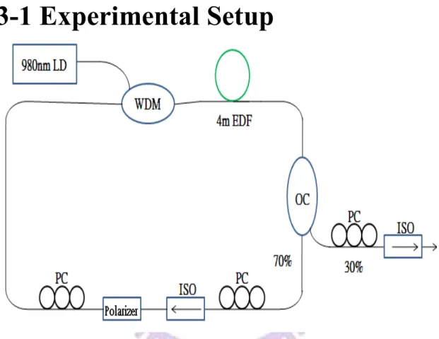
Fig. 3.1 Experimental setup of the passive mode-locked fiber laser.

Our experiment setup is illustrated in Fig. 3.1. We use a fiber ring laser

mode-locked through the nonlinear polarization evolution (NPE) mechanism. The NPE effect, when followed by intensity discrimination with a polarization splitter, can provide ultrafast effective saturable absorption for mode-locking. The all-fiber ring laser cavity utilizes a 4-m-long erbium-doped fiber with 980-nm LD pumping as the gain

37

medium. The ring includes an optical isolator (ISO) that ensures unidirectional laser emission at 1.55 um. It also has two polarization controllers, which are used to adjust the polarization of the light. The cavity length is 10m, composed by 4m Er-doped fiber and 6m SMF-28. The output coupler is 70/30 with 70% returning back to ring and 30% used for the laser output. The total cavity GVD of the laser is in the anomalous dispersion regime.

3-2 Laser characteristics

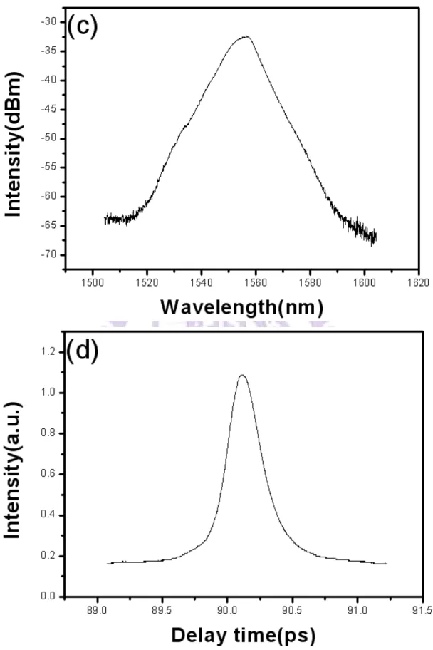
Our laser system can operate under two different states: soliton and chaotic. A striking feature of the laser is that by simply changing the orientation of the polarization controllers, the soliton laser operation state could be changed into a new mode-locked state with a different optical spectrum of broad bandwidth. The broadband spectrum suggests that the laser is still mode-locked. However, its spectral distribution is very different to that of the soliton operation state. The soliton spectrum has symmetric Kelly sideband as in Fig. 3.2(a) and the auto-correlation trace is shown in Fig. 3.2(b). Fig. 3.2(c) shows the smooth and broadband optical spectrum under the chaotic state. The auto-correlation trace under the chaotic state is shown in Fig. 3.2(d).

39

Fig. 3.2(a) Optical spectrum under the soliton state, 3dB bandwidth: 10nm, span: 50nm. (b) Auto-correlation trace under the soliton state, pulse width: 311fs. (c) Optical spectrum

under the chaotic state, 3dB bandwidth: 12nm, span: 100nm. (d) Auto-correlation under the chaotic state, pulse width: 308fs.

40

Fig. 3.3 shows the RF intensity spectra and the phase noise spectra for both the soliton and chaotic states. Fig 3.3 (a) and Fig 3.3 (d) indicate that the laser repetition rate is close to 20MHz, which is the fundamental cavity repetition frequency. The RF signal is 60dB above the noise background under the soliton state. However, the intensity noises are obviously larger in Fig. 3.3(e) for the chaotic state. The resulting phase noise spectra of the two states are shown in Fig. 3.3(c) and Fig. 3.3(f). The chaotic state possesses ultrahigh phase noises about -40 dBc/Hz at the low frequencies. There is also a noise bump around 100kHz. The noise level drops to -120 dBc/Hz at 10MHz eventually.

43

Fig. 3.3 (a) RF spectrum under soliton state; span 100MHz. (b) RF spectrum under soliton state; span 10MHz. (c) Phase noise measurement under soliton state. (d) RF spectrum under chaotic state; span 100MHz. (e) RF spectrum under chaotic state;

span 10MHz.(f) Phase noise measurement under chaotic state.

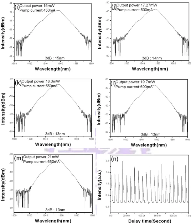
Fig. 3.4 shows that the output power is increasing linearly with the pump current for both states. Experimentally we first tune the polarization controllers into a particular state for either soliton or chaotic operation. Second, we reduce the pump current to zero. Third, we then increase the pump current gradually without changing the orientation of the polarization controllers. It can be seen that it needs a higher pump current to reach the chaotic mode-locked state (430mA pump current should be required). In contrast, one only needs 150mA pump current to reach the soliton state.

44

45

To have a better clue for the laser dynamic difference of the two

operation states, we have also recorded the changes of the optical spectra from CW to mode-locked states. When we increase the pump current continuously, Fig. 3.5 shows that there is only one CW peak in the optical spectra before the soliton mode-locking. On the contrary, there are two competing CW peaks at 1530 and 1560 nm before the chaotic mode-locking as shown in Fig. 3.6. Moreover, we observe that the pulse amplitudes in the chaotic pulse train are not the same and randomly varying when measured by a real-time oscilloscope. But they are the same in the soliton case.

Fig. 3.5 (a)~(c)Transition of optical spectra from CWSoliton mode-locked state (d) The pulse train measured by a Lecroy real time oscilloscope.

47

Fig. 3.6 (a)~(m)Transition of optical spectra from CWChaotic mode-locked state (n) the pulse train measured by a Lecroy real time oscilloscope.

48

3-3 Pulse propagation in optical

fibers

3-3-1 Soliton pulse operation state

For the soliton state, Fig. 3.7 shows that the initial pulse width before transmission is 355 fs, and its 3dB bandwidth is 8nm. In Fig. 3.8, we utilize this soliton pulse to propagate through about 20m &100m SMF-28. The results indicate that the autocorrelation trace can still be fitted well by assuming the sec2h profile, and the measured pulse width agrees with the expected value from the straightforward calculation based on the known fiber dispersion: 8(nm)*17(ps/nm*km)*0.02(km)=2.7ps. The expected pulse broadening indicates that the nonlinear effect is not enough and thus the outcome is mainly dispersion dominated.

Fig. 3.7 (a)Auto-correlation trace before 20m & 100m SMF-28 propagation under soliton state, FWHM: 355fs(b) Optical spectrum before 20m & 100m SMF-28 propagation under

49

Fig. 3.8 Auto-correlation trace after 20m & 100m SMF-28 propagation under soliton state(up), FWHM: 2.77ps and sec2h curve fitting schematic diagram in 20 m SMF

50

3-3-2 Chaotic pulse operation state

For the chaotic pulse state, Fig. 3.9 shows that the initial pulse width before transmission is 308 fs, and its 3dB bandwidth is 14nm. In Fig. 3.10, we utilize the chaotic pulse to propagate through 20m & 100m SMF-28. After propagation, we can observe that there are a narrow central spike and a broad base in the auto-correlation trace. This broad base can be affected by dispersion. If we propagate the pulse train through longer length SMF-28, the broad base will be more broaden and the central peak will be lower. However the width of the central narrow spike is not much affected by the fiber length. This is a signature indicating that the laser may output a chaotic pulse train.

Fig. 3.9 (a)Auto-correlation trace before 20m & 100m SMF-28 propagation under chaotic state, FWHM: 308fs(b)Optical spectrum before 20m & 100m SMF-28 propagation under

51

Fig. 3.10 Auto-correlation trace after 20m & 100m SMF-28 propagation under chaotic state(up)and sec2h curve fitting schematic diagram in 20m SMF propagatio(down)

52

We then use a bandpass filter to keep only the central spectrum band because we want to verify if the mode-locking quality of the central spectral part could be better. Fig. 3.11 gives the optical spectrum and the auto-correlation after the bandpass filter. Here the band-pass filter is with a square profile. In Fig. 3.12, we utilize the filtered pulses to propagate through 20m SMF-28 again and get the same result as in Fig. 3.10. From these data, we can conclude that chaotic mode-locking quality is over the whole optical spectrum.

Fig. 3.11 (a)Auto-correlation trace after band-pass-filter under chaotic state, FWHM: 601 fs(b)Optical spectrum after band-pass-filter under chaotic state, 3dB bandwidth:

53

Fig. 3.12 Auto-correlation trace after 20m BPF&SMF-28 propagation under chaotic state(up)and sec2h curve fitting schematic diagram(down).

54

3-4

Four-wave

mixing

and

super-continuum generation

In this section, we compare the difference of nonlinear pulse propagation for the soliton case with the Kelly sidebands or without the Kelly sidebands. First we let the laser operate under the soliton state as in Fig. 3.13. Then we set up two comparative experiments. The first case is with the optical spectrum as shown in Fig. 3.14, in which the Kelly sidebands have been filtered out by the band-pass-filter. From the auto-correlation trace, the FWHM pulse-width is 599fs. The other case is obtained by connecting a VOA (variable optical attenuator) to form 600fs-pulse width as in Fig. 3.15. The VOA is for adjusting the output power to let both the input average power and pulse-width are roughly the same before the dispersion-shifted-fiber. In the next step we propagate the 600 fs short pulses of the two cases through several hundred meters of the dispersion shifted fiber (DSF). The DSF can provide larger nonlinear effects than the SMF-28. Fig 3.16 shows the evolution of the optical spectrum and auto-correlation trace with linearly increasing power levels for the case without Kelly sidebands. One can observe that the shorter-wavelength band grows up with the increasing output power due

55

to the four-wave-mixing effects. On the other hand, Fig. 3.17 shows the results for the case with Kelly sidebands. One can see a more significant walk-off effect in the auto-correlation measurement for the higher optical power levels. The reason may be because the Kelly sidebands can be a more effective energy intermediary between the two spectral bands (1530 & 1560 nm).

Fig. 3.13 (a) Optical spectrum (3dB bandwidth: 10nm) and (b) auto-correlation trace (FWHM: 306fs) under the soliton state.

Fig. 3.14 (a) Optical spectrum and (b) auto-correlation trace (FWHM: 599fs ) after band-pass filtering under the soliton state.

56

Fig. 3.15 (a)Optical spectrum and (b)auto-correlation trace (FWHM: 600 fs ) after VOA under the soliton state.

57

Fig. 3.16 (a)~(n) Evolution of optical spectrum and auto-correlation trace after BPF & DSF on different power levels under the soliton state without Kelly sidebands.

59

Fig. 3.17 (a)~(p)Evolution of optical spectrum and auto-correlation trace after VOA & DSF on different power levels under the soliton state with Kelly sidebands.

60

As a comparison, we then perform the following experiments by utilizing the chaotic mode-locked state. We propagate the chaotic pulse train through the dispersion-shifted-fiber to generate super-continuum. Fig. 3.18 shows the optical spectrum of the chaotic pulses with the central wavelength of 1552 nm and the spectral width of 13 nm. The FWHM pulse-width from the auto-correlation trace is 300 fs and the laser output power is 24mW. Fig. 3.19 is the super-continuum generation result after propagating through the dispersion shifted fiber. The most interesting point is that there is no significant modulation on the super-continuum spectrum when we raise the optical power to extend the optical spectrum. The 3dB bandwidth can reach ~120nm with a relatively uniform spectral distribution. It can be used as a broadband light source which can find many useful applications.

Fig. 3.18 (a) Optical spectrum under the chaotic state, 3dB bandwidth: 13nm, span: 100nm. (b) Auto-correlation trace under the chaotic state, pulse width: 300fs.

61

Fig. 3.19 Super-continuum generation after DSF propagation under the chaotic state (3dB bandwidth: 120nm).

62

3-5 Pulse compression

In this section, we try to compress the generated ultra-short pulses to achieve the possible minimum pulse-width and to implement the pulse compression experiment for comparing the soliton and chaotic states.Fig. 3.20 shows the schematic diagram for the pulse compression experiment, including a band-pass optical filter, EDFA, and a section of SMF-28 for the dispersion compensation.The optical filter is used only for the soliton state because we want to filter out the kelly sideband in order to obtain a more clean optical spectrum. First we let the laser operate in the soliton state, which has the spectral width of 10nm and pulse-width of 305 fs in Fig.3.21. Then we use the band-pass filter to filter out the Kelly sideband spectral part as in Fig. 3.22, which produces the FWHM pulse-width =596 fs, estimated from the auto-correlation trace. In the next step we connect an EDFA to provide the normal dispersion. Fig. 3.23 also shows that there are some nonlinear effects caused by the EDFA since the optical spectrum bandwidth is broaden to 13nm. Finally we choose the 6m SMF to be the compressor for the soliton state case, which is experimentally the most optimized length to compensate the pulse chirp caused by the nonlinear effects and normal dispersion of the EDFA.

63

When we increase the EDFA pumping current, we can observe that the EDFA output power is proportional to the optical spectrum broadening but inversely proportional to the auto-correlation trace width in Fig. 3.24. Eventually, the minimum pulse-width we obtain is 223 fs and the broadened spectrum bandwidth is about 50nm.

Fig. 3.20 Schematic diagram of pulse compression

Fig. 3.21 (a) Optical spectrum and (b) auto-correlation trace under the soliton state. Spectral 3dB bandwidth: 10nm, span: 50nm, FWHM pulse-width: 305fs.

Fig. 3.22 (a) Optical spectrum and (b) auto-correlation trace after band-pass filtering under the soliton state. Span: 50nm, FWHM pulse-width: 596 fs.

64

Fig. 3.23 (a) Optical spectrum and (b) auto-correlation trace after BPF&EDFA under the soliton state. Spectral bandwidth:13nm, span: 50nm, FWHM pulse-wdith: 966 fs.

66

Fig. 3.24 (a)~(v) Evolution of optical spectrum and auto-correlation trace after BPF&EDFA by increasing the output power under the soliton state

67

Again, as a comparison, we let the laser operate in the chaotic state, which exhibits the spectral width of 12nm and the pulse-width of 308 fs as shown in Fig. 3.25. After the EDFA, we find that the 3dB spectrum bandwidth does not exceed the original 3dB bandwidth even we continuously enhance the EDFA pumping current. We also observe that there is no significant modulation on the optical spectra.Furthermore, we find that the auto-correlation trace is with a narrow central spike and a broad base for the chaotic state, as shown in Fig. 3.26. Finally we set the output power to be 16.2 mW as the case in Fig. 3.27. Then we use 2m, 6m, 8m, and 9m of SMF-28 to compress the chaotic pulse. The narrow central coherence spike is not affected by the linear dispersion compensation, indicating that the chaotic pulses cannot be compressed well.

Fig. 3.25 (a) Optical spectrum and (b) auto-correlation trace under the chaotic state. 3dB bandwidth: 12nm, span: 100nm, FWHM pulse-width: 308fs.

69

Fig. 3.26 Evolution of optical spectrum and auto-correlation by increasing the EDFA output power under the chaotic state.

Fig. 3.27 Auto-correlation trace after EDFA under the chaotic state. Output power: 16.2 mW.

71

Fig. 3.28 Auto-correlation traces after EDFA & (a) 2m, (b) 6m, (c) 8m, and (d) 9m SMF under the chaotic state.

72

Chapter 4

Conclusion and future work

4-1 Summary of the achievements

We have experimentally observed two kinds of passive mode-locked laser operation states (soliton and chaotic-like) with the use of the P-APM technique. The soliton operation state is with some symmetric kelly sidebands while the chaotic pulse operation state exhibits a smooth broad spectrum. Both states can produce ultrashort pulse trains with the FWHM pulse-width around 300 fs. However, the pulse characteristics of the two states become very different after propagating through additional optical fibers. From the results after propagating through the DSF under the soliton operation, we can observe obvious four-wave-mixing effects on the optical spectrum and obvious walk-off effects in the auto-correlation trace with the presence of Kelly sidebands. By propagating the chaotic pulses through the DSF, we can obtain a super-broadband light source. Its bandwidth can reach 120nm with a relatively uniform spectral distribution. This can be an advantageous application for the observed chaotic operation state.

73

We have also investigated the possibility of performing further pulse compression to reduce the pulse-width for both states. An EDFA with normal dispersion and a section of SMF-28 are used as the compressor. The minimum possible pulse-width is 223 fs under the soliton operation. However, the chaotic pulse train exhibits a narrow central coherence spike which is not affected by the dispersion, indicating that the chaotic pulse train cannot be compressed well.

Finally, the comparative experiment in the literature shows that broadband super-continuum lights can be generated by noise-like pulses propagating in a section of 100m standard single-mode-fiber operated in the normal dispersion regime [4.1].The super-continuum exhibits a pulse energy threshold of 43 nJ (corresponds to ~1 W of the average power) and a flat spectrum over 1050-1250 nm. On the contrary, we just use 24mW of the average power to reach a 120 nm relatively flat spectral distribution after propagating through the DSF. From such comparison, the chaotic ultra-short pulse operation state investigated in the present work may find useful applications for super-continuum generation.

74

4-2 Possible future work

In principle, there are at least three points that we may try to improve or implement in the future.

(1) We can try to further improve the performance of super-continuum generation. In order to obtain more nonlinear effects on pulse propagation, using the HNLF or adding a higher power optical amplifier after the laser output can be the method.

(2) In Fig. 3.6, if we use two band-pass filters to selectively separate the spectral components around 1530nm and 1550nm so as to measure them individually by an oscilloscope, we may be able to test the intensity correlation between the two spectral components. The obtained results may help to clarify whether the coexistence of the 1530nm and 1550nm CW lasing under the lower pumping power is indeed the key for the existence of the chaotic mode-locked state under the higher pumping power.

(3) In the literature, the chaotic (noise-like) mode-locked states are all found in passive mode-locked laser systems. It is interesting to see if we can use a modulator to achieve a high repetition rate chaotic mode-locked fiber laser.

75

References

[4.1] A. Zaytsev, C. H. Lin, Y. J. You, C. C. Chung, C. L. Wang, and C. L. Pan, “Super-continuum generation by noise-like pulses transmitted

through normally dispersive standard single-mode fibers,” Opt.

Express, vol. 21, pp. 16056-16062, 2013.