國
立
交
通
大
學
電機學院 電子與光電學程
碩
士
論
文
適用於 H.264/AVC 之降低記憶體頻寬的動作補償
A Memory Bandwidth-Reduction Motion Compensator for
H.264/AVC Application
研 究 生:陳浩民
指導教授:李鎮宜 教授
適用於 H.264/AVC 之降低記憶體頻寬的動作補償
A Memory Bandwidth-Reduction Motion Compensator for
H.264/AVC Application
研 究 生:陳浩民 Student:Hao-Min Chen
指導教授:李鎮宜 Advisor:Chen-Yi Lee
國 立 交 通 大 學
電機學院 電子與光電學程
碩 士 論 文
A ThesisSubmitted to College of Electrical and Computer Engineering National Chiao Tung University
in partial Fulfillment of the Requirements for the Degree of
Master of Science in
Electronics and Electro-Optical Engineering December 2010
Hsinchu, Taiwan, Republic of China
適用於 H.264/AVC 之降低記憶體頻寬的動作補償
學生:陳浩民 指導教授:李鎮宜 教授
國 立 交 通 大 學 電 機 學 院 電 子 與 光 電 學 程 碩 士 班
摘
要
近年來,對於已被數位 視訊廣播的高傳真電視廣播服務 和藍光光碟所採用的
H.264/AVC High Profile 視訊標準,其需求是很必要的。而動作補償單元的計算量通常占 了整個視訊解碼系統的大多數,這是由於它需要對參考畫面的記憶體有相當大量的資料 傳輸。特別在目前最先進的 H.264/ AVC Main/High Profile 視訊標準支援了雙向參考畫
面,因而使得所需的記憶體頻寬大量增加。我們提出的記憶體頻寬縮減策略除了可有效 地減少所需的記憶體頻寬高達 80 %之外,同時維持和整個視訊解碼系統相同的解碼順
序。和傳統的架構相較之下,針對 H.264 提出的可重新架構的內插器,可省下 20 % 的 邏輯閘數量。我們的動作補償單元同時支援了 H.264 Baseline Profile @ 4.0 Level 和
H.264 Main/High Profile @ 4.0 Level,對即時解碼能力而言可達到 1080 HD @ 100.0 MHz,而總邏輯閘數量為 68 K。
A Memory Bandwidth-Reduction Motion Compensator for
H.264/AVC Application
Student : Hao-Min Chen Advisor : Dr. Chen-Yi Lee
Degree Program of Electrical and Computer Engineering
National Chiao Tung University
ABSTRACT
In recent years, H.264/AVC High Profile video standard, which has been adopted by the
Digital Video Broadcasting (DVB) HDTV broadcast service and the Blu-ray Disc storage format, is necessary in demand. The computation time of motion compensation unit is usually
accounted for most of the video decoding system because of the enormous data transfer with reference frame memories. Particularly in the most advanced H.264/AVC Main/High Profile
video standard supports bi-prediction reference frame, which makes the memory bandwidth required for a significant increase. Our proposed reduction strategies of memory bandwidth
cannot only effectively reduce the required memory bandwidth up to 80% but also maintaining the same decoding order as that of entire video decoding system. The proposed
restructured interpolator can save 20% of the number of logic gates compared to traditional design. Our motion compensator also support H.264 Baseline Profile @ 4.0 Level and
Main/High Profile @ 4.0 Level, in terms of real-time decoding up to 1080 HD @ 100 MHz, while the total number of 68k NAND2 CMOS logic gate count.
Acknowledgements
首先要感謝的是我的指導教授李鎮宜研發長在我的碩士生涯中給我的指導與鞭 策,在他熱心指導過程中,雖然常常我有很爆笑的回應,但總是能很有耐心的指導我。 接下來要感謝,帶領我的博士班學長,也是我們 Si2 多媒體組 leader 李曜,在他有 效的領導與熱心的幫助,讓我的研究持續有進展;另外要感謝王勝仁學長,他的論文非 常優秀,很值得我借鏡,對我的研究幫助很大;接下來要感我們 Si2 實驗室的成員們, 耀琳,謝謝你為了教我 ICLAB 常常陪我熬夜;還有見縫就插針的的明瑜;要把好的 idea 分給我的建辰;分享酒店文化的義澤,分享把妹經驗的人偉;常常幫我介紹的勝舜;下 課常一起聊天的元雍與盈鋒;老是說真的的長宏;常回來的子明學長;老是叫我捐錢的 欣儒;大家一起做研究,一起敖夜,一起唱歌,一起聊天,一起聚餐。在苦悶的研究生 涯帶來了豐富的歡樂色彩。 最後要感謝的是我的家人,強列的要求我再進修,也由於有他們的支持,讓我可 以在沒有後顧之憂的,全心完成我的研究。Contents
CHAPTER 1 INTRODUCTION ... 1
1.1 MOTIVATION ... 1
1.2 THESIS ORGANIZATION ... 2
CHAPTER 2 ALGORITHM DESCRIPTION AND ANALYSIS ... 3
2.1 PROFILING ... 4
2.2 INTER PREDICTION ALGORITHM FOR H.264/AVCSTANDARD ... 5
2.3 INTER PREDICTION FOR H.264/AVCHIGH PROFILE STANDARDS ... 8
2.4 BANDWIDTH REQUIREMENT FOR INTER PREDICTION ... 13
2.5 SUMMARY ... 14
CHAPTER 3 MOTION COMPENSATION DESIGN FOR H.264/AVC MAIN/HIGH PROFILE VIDEO DECODER ... 15
3.1 MOTION COMPENSATION ENGINE FOR H.264/AVC DECODER ... 16
3.2 MVG SUPPORT MAIN/HIGH PROFILE ... 17
3.3 INTERPOLATOR DESIGN ... 26
3.3.1 Luma Interpolator Design ... 26
3.3.2 Chroma Interpolator Design ... 31
3.3.3 Combine Luma and Chroma FIR Design ... 33
3.4 WEIGHTED PREDICTION... 38
3.5 SUMMARY ... 41
CHAPTER 4 MEMORY BANDWIDTH REDUCTION ... 42
4.1 REDUCTION STRATEGIES OF MEMORY BANDWIDTH... 44
4.1.1 Exact Fetch Necessary Pixels ... 45
4.1.2 Pre-fetch Mechanism ... 47
4.1.3 Intra MB Pixel Reusing ... 49
4.1.4 Inter MB Pixel Reusing... 50
4.2 LIMIT OF REDUCED MEMORY BANDWIDTH ... 52
4.3 SUMMARY ... 55
CHAPTER 5 EXPERIMENT RESULT ... 56
5.1 SYSTEM SPECIFICATION ... 56
5.2 COMPARISON WITH RELATED WORKS ... 61
CHAPTER 6 CONCLUSION AND FUTURE WORK ... 63
6.1 CONCLUSION ... 63
6.2 FUTURE WORK ... 64
List of Figures
FIG 2.1GENERAL STRUCTURE OF H.264 ENCODER ... 3
FIG 2.2GENERAL STRUCTURE OF H.264 DECODER ... 3
FIG 2.3H.264/AVC VIDEO DECODER SOFTWARE PROFILE ON ARM PROCESSOR (JM8.2) ... 4
FIG 2.4MACROBLOCK PARTITIONS AND SUB-MACROBLOCK PARTITIONS ... 5
FIG 2.5(A) LUMA HALF SAMPLE WITH 6-TAP FIR,(B) LUMA QUARTER SAMPLE WITH BILINEAR FILTER,(C) CHROMA SAMPLE WITH BILINEAR FILTER.UPPER-CASE LETTERS INDICATE THE FULL SAMPLES AND LOWER-CASE LETTERS INDICATES THE INTERPOLATED FRACTIONAL SAMPLES ... 6
FIG 2.6(A) DIRECTIONAL PREDICTION FOR 8 X 16 BLOCK SIZE,(B) DIRECTIONAL PREDICTION FOR 16 X 8 BLOCK SIZE,(C) MEDIAN PREDICTION ... 7
FIG 2.7BI-PREDICTION EXAMPLES ... 8
FIG 2.8EXAMPLES OF PREDICTION MODES IN B SLICE MACROBLOCKS ... 9
FIG 2.9 EXAMPLE FOR TEMPORAL DIRECT-MODE MOTION VECTOR ... 10
FIG 2.10INTERLACED VIDEO SEQUENCE ... 12
FIG 2.11MACROBLOCK-ADAPTIVE FRAME-FIELD CODING... 13
FIG 3.1MOTION COMPENSATION ENGINE FOR H.264 VIDEO DECODER ... 16
FIG 3.7MOTION VECTORS INFORMATION STORAGE FOR MOTION VECTOR PREDICTOR FOR QCIF FRAME FORMAT. ... 17
FIG 3.8(A)NEIGHBORING MOTION VECTORS NEEDED WHEN DECODING ALL MOTION VECTORS IN
VERSION ... 19
FIG 3.9MOTION VECTOR GENERATOR ARCHITECTURE FOR QCIF-FORMAT SUPPORT MBAFF ... 20
FIG 3.10 MOTION VECTOR GENERATOR ARCHITECTURE ... 26
FIG 3.11SEPARATE 1-D INTERPOLATOR DESIGN (NO PARALLEL) ... 26
FIG 3.12ONLY ONE HALF PIXEL IS NEEDED ... 28
FIG 3.13ORIGINAL 4-PARALLEL SEPARATE 1-D LUMA INTERPOLATOR ... 29
FIG 3.14ENHANCE 4-PARALLEL SEPARATE 1-D LUMA INTERPOLATOR ... 30
FIG 3.15INTERPOLATION WINDOW FOR EACH 2 X 2 CHROMA BLOCK ... 31
FIG 3.16(A) CHROMA INTERPOLATOR,(B) VERTICAL/HORIZONTAL FILTRR ... 32
FIG 3.172-PARALLEL CHROMA INTERPOLATOR ... 33
FIG 3.18(A) LUMA FIR DESIGN IN CHEN‟S [3],(B) BILINEAR FILTER ... 33
FIG 3.19COMBINED LUMA/CHROMA INTERPOLATOR DESIGN FOR H.264 ... 34
FIG 3.20(A) PATH OF LUMA FIR INTERPOLATOR,(B) PATH OF CHROMA 1/8 BILINEAR ... 35
FIG 3.21ENTIRE INTERPOLATOR ARCHITECTURE ... 36
FIG 3.22WEIGHTED PREDICTOR DESIGN ... 39
FIG 3.23ENTIRE WEIGHT PREDICTOR ARCHITECTURE ... 40
FIG 4.14 X 4 BLOCK WINDOW AND THE CORRESPONDING 9 X 9 INTERPOLATION WINDOW ... 42
FIG 4.8EMBEDDED COMPRESS/DECOMPRESS METHOD ... 44
FIG 4.9 FRACTIONAL SAMPLE POSITIONS FOR QUARTER SAMPLE LUMA INTERPOLATION ... 45
FIG 4.10FRACTIONAL SAMPLE ONLY NEED HORIZONTAL SAMPLES ... 46
FIG 4.11FRACTIONAL SAMPLE ONLY NEED VERTICAL SAMPLES ... 46
FIG 4.12PRE-FETCH MECHANISM ... 48
FIG 4.134X4 BLOCK WINDOW AND THE CORRESPONDING 9X9 INTERPOLATION WINDOW AND OVERLAPPED REGION FOR NEIGHBORING INTERPOLATION WINDOW ... 49
FIG 4.14INTRA MB OVERLAP PIXELS REUSING ... 50
FIG 4.16ALL OVERLAP REGION INCLUDE BETWEEN PREVIOUS UPPER MB AND LEFT MB ... 53
FIG 4.17NO OVERLAP REGION CAN BE REUSED ... 54
FIG 5.1MOTION COMPENSATION ENGINE FOR H.264 VIDEO DECODER ... 57
FIG 5.2SIMULATION RESULTS OF BANDWIDTH REDUCTION STRATEGIES ... 58
FIG 5.3COMPARE RELATED WORKS ... 58
FIG 5.4RATIO OF PIXELS POSITION IN AKIYO AND STEFAN SEQUENCE ... 59
FIG 5.5 LUMA INTEGER/FRACTIONAL MOTION VECTOR PROPORTION FOR H.264/AVC ... 60
List of Tables
TABLE 3.1MEDIAN PREDICTION TABLE IN MBAFF FRAMES... 20
TABLE 3.2 CO-LOCATED MACROBLOCK TABLE ... 24
TABLE 3.3 CO-LOCATED PARTITION TABLE ... 25
TABLE 4.2SUMMARY OF LUMA INTERPOLATION WINDOWS ... 47
TABLE 4.3SUMMARY OF CHROMA INTERPOLATION WINDOWS ... 47
TABLE 4.4STORAGE REQUIREMENT AND LIFETIME ANALYSIS ... 51
TABLE 4.5SUMMARY OF LUMA INTERPOLATION WINDOWS AND REDUCTION PERCENT ... 52
TABLE 4.6SUMMARY OF REDUCTION PERCENT IN DIFFERENT OVERLAP REGION ... 53
TABLE 5.1VIDEO DECODER SPECIFICATION IN OUR DESIGN ... 56
Chapter 1
Introduction
1.1 Motivation
In recent years, the newest video coding standard published jointly as Part 10 of MPEG-4 and ITU-T Recommendation H.264 [1] provides fine video compression
performance. The new H.264/AVC standard provides a technical solution for a wider range of applications, including video-on-demand (VOD), mobile networks, high definition TV,
broadcast over cable, satellite, cable modem, DSL or terrestrial, interactive or serial storage like BD, conversational services over ISDN, Ethernet, LAN, wireless, or mobile network,
multimedia messaging services over DSL, ISDN, etc.
Besides, in Nov. 2004, Digital video broadcasting handheld, DVB-H [5], has mandated
support of Main Profile for H.264/AVC SDTV receivers, with an option for the use of High
Profile. The support of High Profile is mandated for H.264/AVC HDTV decoder. Moreover, high definition TV requires huge data transmission particular in frame memory, a memory
controller that efficiently communicates with frame memory is the most significant over the entire video decoding system. Within the video decoding system, motion compensation
always dominates the total amount of data transmission especially when SDRAM or DDR-SDRAM is adopted as external frame memories. Motion compensation should also
1.2 Thesis Organization
This thesis is organized as follows. The algorithm description and analysis is discussed in Chapter 2. In Chapter 3, the motion compensation engine for H.264/AVC video decoder is
presented firstly. Then, the motion compensation engine for H.264 high profile is illustrated. In Chapter 4, we propose the bandwidth reduction strategies to reduce the required bandwidth
particularly in H.264/AVC integral and fractional motion compensation. We also presents frame memory organization, and memory bandwidth analysis. Implementation result is given
Chapter 2
Algorithm Description and Analysis
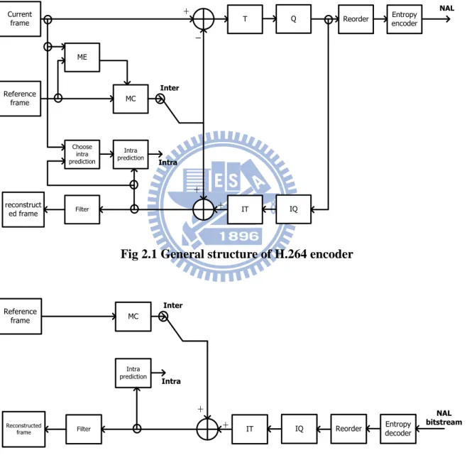
Current frame ME MC Reference frame reconstruct ed frame Choose intra prediction Intra prediction Filter _ + + + T IT Q IQ
Reorder Entropy encoder
NAL
Inter
Intra
Fig 2.1 General structure of H.264 encoder
MC Reference frame Intra prediction Filter + + IT IQ Inter Intra
Reorder decoderEntropy
NAL bitstream
Reconstructed frame
Fig 2.2 General structure of H.264 decoder
Fig 2.1 and Fig 2.2 shows the general structure of H.264/AVC video encoder and
Network Abstraction Layer (NAL). We only discuss on VCL that efficient represents the video content. The concept of H.264/AVC submits the so-called block-based hybrid video
coding. It consists of hybrid of temporal and spatial prediction and is simultaneous with transform coding.
This chapter is structured as follows. The software profiling is illustrated in section 2.1.
Then, the algorithm of H.264/AVC motion compensation would be described in section 2.2. Finally, the H.264/AVC high profile is presented in section 2.3
2.1 Profiling
Fig 2.3 H.264/AVC video decoder software profile on ARM processor (JM 8.2)
7% 8% 9% 7% 9% 9% 8% 11% 32% Others (Intra Prediction, etc.) Write File
PSNR Computation
De-blocking Filter
CAVLC
IQ/IDCT Ref. Frame Copy
Reconstruction
Fig 2.3[8] shows the H.264/AVC profile on ARM processor. The reference software is JM 8.2 [7]. We can find motion compensation related modules, including motion
compensation, reconstruction, and reference frame copy, occupy 51 % proportion of the entire video decoder. Parallel processing, bandwidth reduction, or pipeline processing on ASIC
design can significantly reduce this dominated part.
2.2 Inter Prediction Algorithm for H.264/AVC Standard
H.264/AVC standard supports variable block size (VBS) in inter prediction [1] [2]. The
smallest block size could reach least 4x4 for luma and 2x2 for chroma. Fig 2.4 [1] illustrates all types of partitions.
0 0 0 1 1 0 2 1 3 0 0 0 1 1 0 2 1 3 16x16 16x8 8x16 8x8 8x8 8x4 4x8 4x4 Macroblock partitions Sub-macroblock partitions
Fig 2.4 Macroblock partitions and sub-macroblock partitions
H.264/AVC standard also supports high motion resolution that reaches quarter motion
accuracy for luma sample and one-eighth for chroma sample. Luma half sample interpolation with a 6-tap (1, -5, 20, 20, -5, 1) symmetrical FIR filter and quarter sample interpolation with
bilinear filter are illustrated in Fig 2.5 (a)-(c). The prediction value of chroma component is generated using bilinear interpolator illustrated in Fig 2.5(d), and the displacement can
achieve one-eighth accuracy. From mathematical equations, they are both 2-D interpolation. However, based on hardware implementation, these equations can be divided into two 1-D to
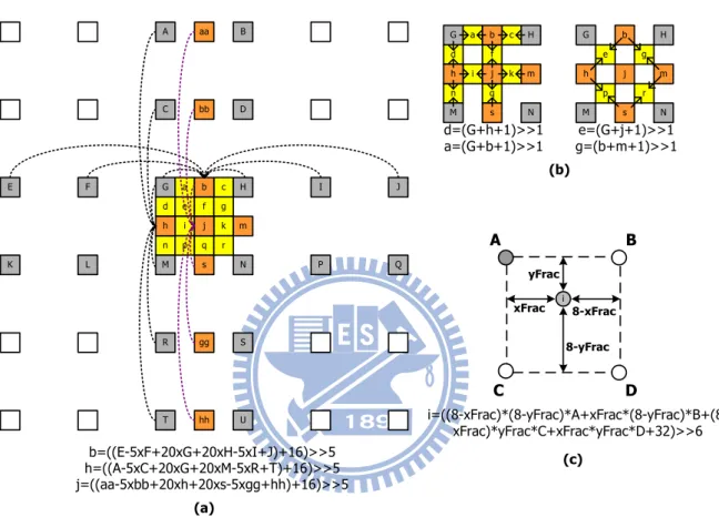
reduce hardware cost, in other words, horizontal filter first and then vertical one, or vice versa. G a c H d n M e i f g k m N p q r I P J Q R S T U B D C A F L E K s h j b bb aa gg hh xFrac yFrac 8-xFrac 8-yFrac A B D C b=((E-5xF+20xG+20xH-5xI+J)+16)>>5 h=((A-5xC+20xG+20xM-5xR+T)+16)>>5 j=((aa-5xbb+20xh+20xs-5xgg+hh)+16)>>5 G H M e g m N p r s h j b e=(G+j+1)>>1 g=(b+m+1)>>1 G a c H d n M i f k m N q s h j b d=(G+h+1)>>1 a=(G+b+1)>>1 (b) i i=((8-xFrac)*(8-yFrac)*A+xFrac*(8-yFrac)*B+(8-xFrac)*yFrac*C+xFrac*yFrac*D+32)>>6 (a) (c)
Fig 2.5 (a) Luma half sample with 6-tap FIR, (b) luma quarter sample with bilinear filter, (c) chroma sample with bilinear filter. Upper-case letters indicate the full samples
and lower-case letters indicates the interpolated fractional samples
Motion vector difference (MVD) and motion vector prediction (MVP) generate the
motion vector which Eq. 2.1 express the equation.
MVPy MVDy MVy MVPx MVDx MVx Eq. 2.1
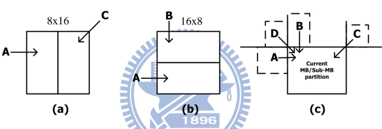
MVD is decoded from bit-stream and MVP is predicted according to neighboring motion vectors. MVP algorithm, contains directional prediction for 16 x 8 or 8 x 16 block size and
median prediction for other block sizes. The detail of MVP decision is shown in Fig 2.6 [8]. Eq. 2.2 expresses the equation of median prediction. Besides, some boundary conditions or
exceptions have to be handled carefully. For instance, when MVC is not available, its value is replaced by MVD. We do not go into detail of those trivial boundary conditions in here.
) , , (MVA MVB MVC median MVP Eq. 2.2 8x16 A C A B Current MB/Sub-MB partition A D B C (a) (b) (c) 16x8
Fig 2.6 (a) Directional prediction for 8 x 16 block size, (b) directional prediction for 16 x 8 block size, (c) median prediction
In addition to the motion-compensated block size described in Fig 2.4, a P macroblock can also be coded to P_SKIP mode. For this coding mode, neither residual signal nor motion
information is transmitted. In other words, motion vectors are only decided according to MVP. The reconstructed reference pixels are obtained similar to macroblock type P_16x16.
Macroblock coded in P_SKIP are often located in large area with no change or slow motion. In addition to the above techniques, H.264/AVC also supports multiple reference frame,
weighted prediction and direct mode for B slice, which we will present in section 2.3. These tools can also improve coding efficiency efficiently.
2.3
Inter Prediction for H.264/AVC High profile Standards
Considering motion compensation, the tools supported by H.264/AVC Main/High Profile are B slices, Weighted Prediction and Interlace video.
In an inter-coded macroblock of B slice, each macroblock partition may be predicted from one or two reference pictures, forward and backward the current picture in temporal
order. This tool provides better coding efficiency with more possibilities to select the best-match prediction references for the macroblock partitions in B slice. Fig 2.7 shows the 3
reference directions: (a) Forward and backward reference pictures, the so-called bi-directional reference, (b) backward reference, and (c) forward references [6]. B slices use two lists of
coded reference pictures, LIST_0 and LIST_1. These two lists can include backward and/or forward coded pictures respectively.
B
(c) two forward (b) two backward
(a) forward and backward
In B slice, there are four prediction modes: (a) direct mode, (b) LIST_0 mode, (c) LIST_1 mode, and (d) bi-predictive mode. For a macroblock, each partition can choose
different prediction modes. When the 8 x 8 partition size is used, the chosen mode for each 8x8 partition is applied to all sub-partition within that partition. Fig 2.8 shows two examples
of prediction mode combinations. In Bi-predictive mode, two motion-compensated reference regions are obtained from LIST_0 and LIST_1 picture respectively. The motion vectors from
LIST_0 and/or LIST_1 in a bi-predictive macroblock or block are predicted form neighboring motion vectors with the same temporal direction. For instance, a motion vector from the
current macroblock pointing to a forward picture is predicted from other neighboring vectors that also point to forward pictures.
Bi pred Bi-pred L1 L1 Direct L0
Fig 2.8 Examples of prediction modes in B slice macroblocks
Similar to the skipped P macroblock coded in P_SKIP mode, a B macroblock can also be
coded in direct mode. In direct mode, no motion vector is transferred for a B slice macroblock or macroblock partition encoded. Instead, the decoder predicts the motion vectors of LSIT_0
and LIST_1 with neighboring vectors and carries out bi-predictive motion compensation block. There are spatial and temporal mode can be used to calculate the LIST_0 and LIST_1
motion vectors for direct mode macroblocks or partitions.
Spatial direct mode is similar to P_SKIP mode. Furthermore, it supports bi-prediction
However, some conditions or exceptions have to be handled carefully. For example, in case of the co-located MB or the partition in the picture that contains the co-located macroblock has a
motion vector that is less than +/- 1/2 luma samples in magnitude (and in some other conditions), one or both of the predicted vectors are set to zero. We do not go into detail of
those trivial conditions here.
Temporal direct mode differs from P_SKIP mode. The same with the spatial direct mode,
the block size is also 4 x 4 block size accuracy, the motion vectors mvL0, mvL1 are derived as scaled versions of the motion vector mvCol of the co-locate sub-macroblock partition. The
scaled method is based on the picture-order-count (POC) distance between the current and LIST_1/LIST_0 picture. Fig 2.9 shows the illustration of temporal direct-mode motion vector
inference. When the object is constant velocity motion, it is suitable-coded in temporal direct mode. When the object is the average form backward and forward, it is suitable-coded in
spatial direct mode. When the object is still, it is suitable-coded in skip mode. Encoder can use skip/direct mode to save one/two motion vector differences (mvd) in every skip/direct
mode partition for further enhance compression efficiency.
List 1 reference List 0
reference
Distance of picture order count MV L0 MV L1 Current picture time MV co-located
Another tool supported in Main/High Profile is Weighted Prediction (WP), which is a method of scaling the samples to increase the video quality in H.264/AVC video decoding. An
application of weighted prediction is to control the relative weighted of interpolated regions to the motion compensated prediction process. For example, WP may be effective in coding of „fade‟ transitions (where one scene fades into another). There are three modes in Weighted
Prediction. When Default mode is in use, two motion compensated reference regions are
obtained from LIST_0 and LIST_1 picture respectively and each sample of the prediction block is calculated as an average of the LIST_0 and LIST_1 prediction samples. Eq. 2.3
expresses the equation
( 0 1 1) 1
p r e d P a r t p r e d P a r t L p r e d P a r t g L Eq. 2.3
When explicit or implicit mode is in use, Eq. 2.4 is used to calculate the sample of the prediction block. The difference between explicit and implicit mode is the weighting factors
are calculated based on the picture-order-count distance between LIST_0 and LIST_1 reference pictures in implicit mode. It is similar to temporal direct mode in motion vector
prediction. When explicit mode is in use, the encoder determines weighting factors. In other words, implicit mode objection is to save weighted prediction parameter in bit-stream for
further enhance compression efficiency.
lo g
0 1 0 1
( ( 0 * 1 * 2 W D) ( lo g 1) ) ( ( 1) 1) )
p r e d P a r t p r e d P a r t L w p r e d P a r t L w W D o o Eq. 2.4
As for interlace video tool, video signal may be sampled as a sequence of complete
frames or interlaced fields. An interlaced video sequence contains a series of fields. A field consists of either the odd-numbered or the even-numbered lines within a complete video
frame. Fig 2.10 illustrates the fields in video sequence. Half of the data in a complete video frame is represented as a field and is sampled at each temporal interval. The advantage of
interlaced video coding is that it is possible to send twice as many fields per second as the number of frames in an equal progressive sequence with the same data rate, giving the
appearance of smoother motion. For instance, a NTSC video sequence consists of 60 fields per second and, when played back, motion can appears smoother than in an equivalent
progressive video sequence containing 30 frames per second.
top field top field bottom field bottom field
Fig 2.10 Interlaced video sequence
Frame coding is more efficient than field coding for progressive video and static pictures in interlaced video. Oppositely, field coding is more efficient for moving pictures in interlaced
video. However, sometimes not complete frames are fast moving. Hence, H.264/AVC Main/High profile provides another tool in interlaced video, macroblock-adaptive frame/field
(MBAFF), to provide macroblock level interlacing. Similar to MBAFF, the picture level interlacing sometimes is called PicAFF. As an extension of PicAFF, MBAFF is used to
improve coding efficiency of picture with both static and moving regions [21]. In MBAFF mode, the current slice is processed in units of 16 luma samples wide and 32 luma samples
choose to encode each MB pair as (a) frame macroblock pair (b) field macroblock pair and may select the optimum coding mode for each region of the picture.
32 16 16 16 16 MB pair 16 16 16 32 16 MB pair
(a)frame MB mode (b)field MB mode
Fig 2.11Macroblock-Adaptive Frame-Field Coding
2.4 Bandwidth Requirement for Inter Prediction
Up to now, we can find interpolation issue becomes more and more important in
state-of-the-art video coding. The interpolation window becomes double for the same block; In other words, it requires double cycles to interpolate each macroblock. For instance, it
requires two 9 x 9 interpolation windows to interpolate a luma 4 x 4 block and four 3 x 3 interpolation windows to interpolate two chroma 2 x 2 blocks in B macroblock.
In worst case, interpolator needs 398MB/s in P frame, 796MB/s in B frame when supporting 1920 x 1088 30fps. In other words, motion compensation needs huge memory
bandwidth requirement. Huge data also means large power consumption for bus activity and data operation.
To reduce bandwidth requirement from frame memory, strategies of memory bandwidth reduction for motion compensation will be proposed in Chapter 4.
2.5 Summary
From the H.264/AVC profiling on ARM processor, an efficient hardware accelerator or
ASIC design for motion compensation is important. The inter prediction for H.264/AVC Baseline, Main/High profiles, and the bandwidth requirement are also illustrated in this
Chapter 3
Motion Compensation Design for
H.264/AVC Main/High Profile video
decoder
The state-of-the-art video coding standard H.264/AVC provides better compression ratio that significantly outperforms all previous video compression standards. However,
H.264/AVC supports Main/High profile and provides many tools compare with Baseline Profile for further enhance compression ratio. Therefore, a development of combining
multi-video coding profiles is essential to support modern multimedia systems. Therefore, it is the challenge of designing efficient video decoder for multi-profile video application
without significantly increase complexity.
This chapter will discuss that designing of motion compensation, which dominates the
amount of data transfer on the H.264/AVC video decoder. The rest part is structured as follows. Section 3.1 illustrates motion compensation engine for H.264/AVC decoder. The
combined motion compensation engine for H.264/AVC Baseline/Main/High profile and the analysis is discussed in section 3.2. Finally, summary is given in section 3.3.
3.1 Motion Compensation Engine for H.264/AVC decoder
Fig 3.1 Motion compensation engine for H.264 video decoder
Fig 3.1 illustrates the whole motion compensation engine for H.264/AVC video decoder. Firstly, Motion vector generator generates motion vector according to motion data. Then, the
address generator uses motion vector with reduction strategies of memory bandwidth to generate address of reference region. Moreover, transfer reference address to system memory
controller (also named well-known arbiter). The tasking of memory access controller is scheduling consecutive access command and sending to frame memories. The burst read data
is kept in read data buffer and then filtered through interpolator. Finally, the interpolated reference data pass through Weighted Predictor to produce motion compensation result. The
result will be added to the residual data and then pass through de-blocking filter. In our proposed decoder, ping-pong structured external frame memory [9], double memories stored
reference and current frame reciprocally, is adopted.
The following subsection will discuss the detail of other modules except reduction
strategies of memory bandwidth. The detailed discussion of reduction strategies of memory bandwidth are shown in Chapter 4. Subsection 3.2 illustrates motion vector generator (MVG)
Supports Main/High Profile including motion vector predictor and the related storages. Subsection 3.3 combines luma and chroma interpolator design. Subsection .3.4 shows
Weighted Predictor design. Finally, summary is presented in section 3.5
3.2 MVG support Main/High profile
Frame boundary Frame boundary …… 0 Top 0 Bot. 1 Top 1 Bot. 2 Top 2 Bot. 3 Top 3 Bot. 4 Top 4 Bot. 5 Top 5 Bot. 7 Top 7 Bot. 6 Top 6 Bot. 8 Top 8 Bot. 9 Top 9 Bot. 10 Top 10 Bot. 11 Top
11 Bot. Current Bot. MB 24 Current
Top MB Next MB 0 Top
Next MB 0 Bot.
Next MB
1 Top Next MB 2 Top
Next MB
1 Bot. Next MB 2 Bot.
Next MB
3 Top Next MB 4 Top
Next MB
3 Bot. Next MB 4 Bot.
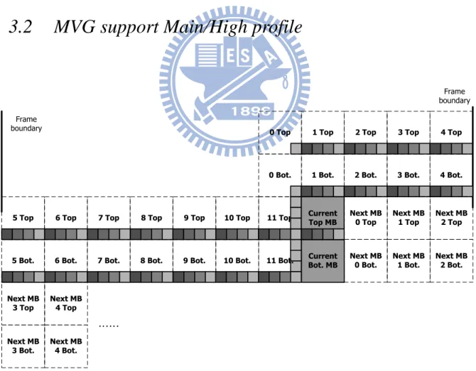
Fig 3.2 Motion vectors information storage for motion vector predictor for QCIF frame format.
There are two tools in MVG for supported Main/High profile. The first one is B slice
type, which has double motion vectors. The second one is MBAFF mode. In MBAFF mode, the handle of macroblock is Macroblock pair. The same with P slice, the required total storage
for motion vector generator, Fig 3.2 shows an example. Total amount of 4 x 11 x 2 both components of the motion vector have to be stored for QCIF frame format. Fig 3.3 (a) shows
the detail of required neighboring motion vectors. To decode T0-T15 in current top MB, it needs neighboring motion vectors in left (TL0-TL3, MVL0-MVL3), above (TU0-TU3,
MVU0-MVU3), above-right (TRU, MVRU), and above-left (TLU-MVLU) position. The 4 x 8 size of MV buffers is required because the maximum number of motion vector per MB pair
is thirty-two. If we reuse the same 4 x 4 size of MV buffers and add a number of buffers (T10, T11, T14, and T15), the MV buffers can be further reduced. Fig 3.3 (b) shows the reduced
T7 T6 T5 T4 T13 T12 T3 T2 T1 T0 T9 T8 TL0 TL1 TL2 BRU BU0 BU1 BU2 BU3
B7 B6 B5 B4 B15 B14 B13 B12 B3 B2 B1 B0 B11 B10 B9 B8 BL0 BL1 BL2 BLU TL3 BL3
TLU TU0 TU1 TU2 TU3 TRU
T10 T11 T14 T15
TL0
TL1
TL2
MVRU MVU0 MVU1 MVU2 MVU3
MV7 MV6 MV5 MV4 MV15 MV14 MV13 MV12 MV3 MV2 MV1 MV0 MV11 MV10 MV9 MV8 MVL0 MVL1 MVL2 MVLU TL3 MVL3 T10 T11 T14 T15
TLU TU0 TU1 TU2 TU3 TRU
Fig 3.3 (a) Neighboring motion vectors needed when decoding all motion vectors in current MBAFF macroblock, (b) reduced and combined with non-MBAFF version
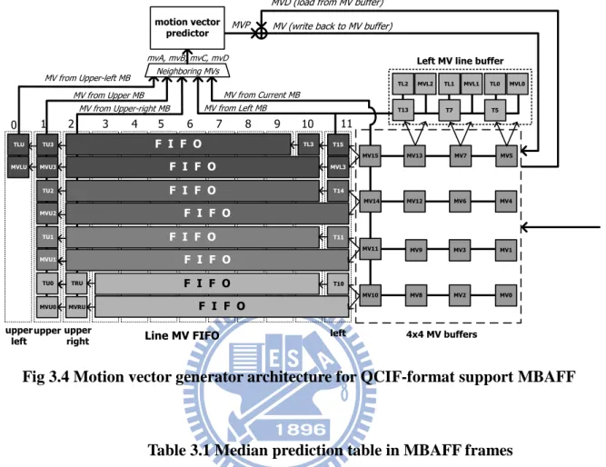
Fig 3.4 shows the detailed architecture of motion vector generator. This architecture
combine non-MBAFF and MBAFF mode. When operation in non-MBAFF TX (with X being 5, 7, 13, 15, and so on) storages can be closed for saving power. The same with P slice, Table
3.1 lists all MVA, MVB, MVC, and MVD for different block size_position index. The difference is MBAFF mode not only size_position index but also current MB pair is
Frame/Field coding, current MB is Top/Bottom MB, and relative MB pair is Frame/Filed coding. Therefore, LUT in MBAFF mode is eight times complexity than non-MBAFF mode.
For cost and area efficiency consideration, we combine MBAFF and non-MBAFF LUT. Fortunately, we can find the condition of MVA, MVB, MVC, and MVD is the same with
non-MBAFF mode when condition of MBAFF mode is fixed in current MB pair is Field, current MB is Bottom MB, and relative MB pair is Field. As mentioned above, we can use the
same LUT to deal with non-MBAFF and MBAFF mode.
4x4 MV buffers Left MV line buffer
MVP
MVD (load from MV buffer) MV (write back to MV buffer)
Line MV FIFO
0 1 2 3 4 5 6 7 8 9 10 11
upperupper left
right mvA, mvB, mvC, mvD MV from Upper MB MV from Left MB MV from Current MB MV from Upper-left MB MV from Upper-right MB Neighboring MVs motion vector predictor MVL0 MVL1 MVL2 MV5 MV7 F I F O MVU3 TLU MV13 MV1 MV3 MV9 F I F O MVU1 MV11 MV4 MV6 F I F O MVU2 MV0 MV2 MV8 F I F O MVU0 MVRU MV10 MV15 MV14 MV12 upper left TL0 T5 TL1 T7 T13 TL2 MVL3 TL3 T15 MVLU TU2 TU1 TU0 TU3 T14 T11 TRU T10 F I F O F I F O F I F O F I F O
Fig 3.4 Motion vector generator architecture for QCIF-format support MBAFF
c u r r e n t M B T /B r e la t iv e M B m v A m v B m v C m v D F r a m e T L 0 B U 0 B U 2 B L U F ie ld F r a m e B L 0 T 1 0 T 1 4 T L 3 F ie ld T L 2 B L 1 F r a m e T L 0 B U 0 B U 2 B L U F ie ld T U 0 T U 2 T L U F r a m T L 0 B U 0 B U 2 B L U F ie ld B L 0 F r a m e T L 1 M V 0 X T L 0 F ie ld T L 0 B L 0 F r a m e B L 1 M V 0 X B L 0 F ie ld T L 2 B L 2 F r a m e T L 2 T 0 X T L 1 F ie ld T L 1 T L 0 F r a m T L 2 B 0 X T L 1 F ie ld B L 1 B L 0 F r a m e M V 1 B U 2 B R U B U 1 F ie ld F r a m e M V 1 T 1 4 X T 1 1 F ie ld F r a m e T 1 B U 2 B R U B U 1 F ie ld T U 2 T R U T U 1 F r a m M V 1 B U 2 B R U B U 1 F ie ld F r a m e M V 3 M V 4 X M V 1 F ie ld F r a m e M V 3 M V 4 X M V 1 F ie ld F r a m e T 3 T 4 X T 1 F ie ld F r a m M V 3 M V 4 X M V 1 F ie ld F r a m e T L 2 M V 2 M V 6 T L 1 F ie ld T L 1 B L 0 F r a m e B L 2 M V 2 M V 6 B L 1 F ie ld T L 3 B L 2 F r a m e B L 0 T 2 T 6 T L 3 F ie ld T L 2 T L 1 F r a m B L 0 M V 2 M V 6 T L 3 F ie ld B L 2 B L 1 F r a m e T L 3 M V 8 X T L 2 F ie ld T L 1 B L 1 F r a m e B L 3 M V 8 X B L 2 F ie ld T L 3 B L 3 F r a m e B L 2 T 8 X B L 1 F ie ld T L 3 T L 2 F r a m B L 2 M V 8 X B L 1 F ie ld B L 3 B L 2 F r a m e M V 9 M V 6 X M V 3 F ie ld F r a m e M V 9 M V 6 X M V 3 F ie ld F r a m e M V 9 M V 6 X M V 3 F ie ld F r a m M V 9 M V 6 X M V 3 F ie ld F r a m e M V 1 1 M V 1 2 X M V 9 F ie ld F r a m e M V 1 1 M V 1 2 X M V 9 F ie ld F r a m e M V 1 1 M V 1 2 X M V 9 F ie ld F r a m M V 1 1 M V 1 2 X M V 9 F ie ld F r a m e T L 0 B U 0 B U 1 B L U F ie ld F r a m e B L 0 T 1 0 T 1 1 T L 3 F ie ld T L 2 B L 1 F r a m e T L 0 B U 0 B U 1 B L U F ie ld T U 0 T U 1 T L U F r a m T L 0 B U 0 B U 1 B L U F ie ld B L 0 F r a m e T o p B o t . F ie l d T o p B o t . F r a m e T o p B o t . F ie l d T o p B o t . F r a m e T o p B o t . F ie l d T o p B o t . F r a m e T o p B o t . F ie l d T o p B o t . F r a m e T o p B o t . F ie l d T o p B o t . F r a m e T o p B o t . F ie l d T o p B o t . F r a m e T o p B o t . 8 x 4 _ 7 4 x 8 _ 0 8 x 4 _ 4 8 x 4 _ 5 8 x 4 _ 6 F ie l d T o p B o t . F r a m e T o p B o t . F ie l d T o p B o t . F r a m e T o p B o t . F ie l d T o p B o t . 8 x 4 _ 0 8 x 4 _ 1 8 x 4 _ 2 8 x 4 _ 3 c u r r e n t M B T /B r e la t iv e M B m v A m v B m v C m v D F r a m e T L 0 B U 0 B R U B L U F ie ld F r a m e B L 0 T 1 0 X T L 3 F ie ld T L 2 B L 1 F r a m e T L 0 B U 0 B R U B L U F ie ld T U 0 T R U T L U F r a m T L 0 B U 0 B R U B L U F ie ld B L 0 F r a m e T L 0 B U 0 B R U B L U F ie ld F r a m e B L 0 T 1 0 X T L 3 F ie ld T L 2 B L 1 F r a m e T L 0 B U 0 B R U B L U F ie ld T U 0 T R U T L U F r a m T L 0 B U 0 B R U B L U F ie ld B L 0 F r a m e T L 2 M V 2 X T L 1 F ie ld T L 1 B L 0 F r a m e B L 2 M V 2 X B L 1 F ie ld T L 3 B L 2 F r a m e B L 0 M V 2 X T L 3 F ie ld T L 2 T L 1 F r a m B L 0 M V 2 X T L 3 F ie ld B L 2 B L 1 F r a m e T L 0 B U 0 B U 2 B L U F ie ld F r a m e B L 0 T 1 0 T 1 4 T L 3 F ie ld T L 2 B L 1 F r a m e T L 0 B U 0 B U 2 B L U F ie ld T U 0 T U 2 T L U F r a m T L 0 B U 0 B U 2 B L U F ie ld B L 0 F r a m e M V 1 B U 2 B R U B U 1 F ie ld F r a m e M V 1 T 1 4 X T 1 1 F ie ld F r a m e M V 1 B U 2 B R U B U 1 F ie ld T U 2 T R U T U 1 F r a m M V 1 B U 2 B R U B U 1 F ie ld F r a m e T L 0 B U 0 B U 2 B L U F ie ld F r a m e B L 0 T 1 0 T 1 4 T L 3 F ie ld T L 2 B L 1 F r a m e T L 0 B U 0 B U 2 B L U F ie ld T U 0 T U 2 T L U F r a m T L 0 B U 0 B U 2 B L U F ie ld B L 0 F r a m e M V 1 B U 2 B R U B U 1 F ie ld F r a m e M V 1 T 1 4 X T 1 1 F ie ld F r a m e M V 1 B U 2 B R U B U 1 F ie ld T U 2 T R U T U 1 F r a m M V 1 B U 2 B R U B U 1 F ie ld F r a m e T L 2 M V 2 M V 6 T L 1 F ie ld T L 1 B L 0 F r a m e B L 2 M V 2 M V 6 B L 1 F ie ld T L 3 B L 2 F r a m e B L 0 M V 2 M V 6 T L 3 F ie ld T L 2 T L 1 F r a m B L 0 M V 2 M V 6 T L 3 F ie ld B L 2 B L 1 F r a m e M V 9 M V 6 X M V 3 F ie ld F r a m e M V 9 M V 6 X M V 3 F ie ld F r a m e M V 9 M V 6 X M V 3 F ie ld F r a m M V 9 M V 6 X M V 3 F ie ld B o t . F r a m e T o p B o t . F ie l d T o p B o t . F r a m e T o p B o t . F ie l d T o p B o t . F r a m e T o p B o t . F ie l d T o p B o t . 1 6 x 8 _ 0 1 6 x 8 _ 1 8 x 1 6 _ 0 8 x 1 6 _ 1 8 x 8 _ 0 F r a m e T o p B o t . F ie l d T o p B o t . F r a m e T o p B o t . F ie l d T o p B o t . F r a m e T o p B o t . 1 6 x 1 6 F r a m e F ie l d T o p B o t . T o p B o t . 8 x 8 _ 2 8 x 8 _ 3 8 x 8 _ 1 F ie l d T o p B o t . F ie l d T o p B o t . F r a m e T o p B o t . F ie l d T o p B o t . F r a m e T o p
c u r r e n t M B T /B r e la t iv e M B m v A m v B m v C m v D F r a m e M V 0 B U 1 B U 2 B U 0 F ie ld F r a m e M V 0 T 1 1 T 1 4 T 1 0 F ie ld F r a m e M V 0 B U 1 B U 2 B U 0 F ie ld T U 1 T U 2 T U 0 F r a m M V 0 B U 1 B U 2 B U 0 F ie ld F r a m e M V 1 B U 2 B U 3 B U 1 F ie ld F r a m e M V 1 T 1 4 T 1 5 T 1 1 F ie ld F r a m e M V 1 B U 2 B U 3 B U 1 F ie ld T U 2 T U 3 T U 1 F r a m M V 1 B U 2 B U 3 B U 1 F ie ld F r a m e M V 4 B U 3 B R U B U 2 F ie ld F r a m e M V 4 T 1 5 X T 1 4 F ie ld F r a m e M V 4 B U 3 B R U B U 2 F ie ld T U 3 T R U T U 2 F r a m M V 4 B U 3 B R U B U 2 F ie ld F r a m e T L 2 M V 2 M V 3 T L 1 F ie ld T L 1 B L 0 F r a m e B L 2 M V 2 M V 3 B L 1 F ie ld T L 3 B L 2 F r a m e B L 0 M V 2 M V 3 T L 3 F ie ld T L 2 T L 1 F r a m B L 0 M V 2 M V 3 T L 3 F ie ld B L 2 B L 1 F r a m e M V 8 M V 3 M V 6 M V 2 F ie ld F r a m e M V 8 M V 3 M V 6 M V 2 F ie ld F r a m e M V 8 M V 3 M V 6 M V 2 F ie ld F r a m M V 8 M V 3 M V 6 M V 2 F ie ld F r a m e M V 9 M V 6 M V 7 M V 3 F ie ld F r a m e M V 9 M V 6 M V 7 M V 3 F ie ld F r a m e M V 9 M V 6 M V 7 M V 3 F ie ld F r a m M V 9 M V 6 M V 7 M V 3 F ie ld F r a m e M V 1 2 M V 7 X M V 6 F ie ld F r a m e M V 1 2 M V 7 X M V 6 F ie ld F r a m e M V 1 2 M V 7 X M V 6 F ie ld F r a m M V 1 2 M V 7 X M V 6 F ie ld F r a m e T L 0 B U 0 B U 1 B L U F ie ld F r a m e B L 0 T 1 0 T 1 1 T L 3 F ie ld T L 2 B L 1 F r a m e T L 0 B U 0 B U 1 B L U F ie ld T U 0 T U 1 T L U F r a m T L 0 B U 0 B U 1 B L U F ie ld B L 0 F r a m e M V 0 B U 1 B U 2 B U 0 F ie ld F r a m e M V 0 T 1 1 T 1 4 T 1 0 F ie ld F r a m e M V 0 B U 1 B U 2 B U 0 F ie ld T U 1 T U 2 T U 0 F r a m M V 0 B U 1 B U 2 B U 0 F r a m e T o p B o t . F ie l d T o p B o t . F r a m e T o p B o t . F ie l d T o p B o t . F r a m e T o p B o t . F ie l d T o p B o t . F r a m e T o p B o t . F ie l d T o p B o t . F ie l d T o p B o t . F r a m e T o p B o t . F ie l d T o p B o t . F r a m e T o p B o t . F ie l d T o p F r a m e T o p B o t . F ie l d T o p B o t . F r a m e T o p B o t . F ie l d T o p B o t . F r a m e T o p B o t . 4 x 8 _ 1 4 x 4 _ 0 4 x 4 _ 1 4 x 8 _ 2 4 x 8 _ 3 4 x 8 _ 4 4 x 8 _ 5 4 x 8 _ 6 4 x 8 _ 7 c u r r e n t M B T /B r e la t iv e M B m v A m v B m v C m v D F r a m e T L 1 M V 0 M V 1 T L 0 F ie ld T L 0 B L 0 F r a m e B L 1 M V 0 M V 1 B L 0 F ie ld T L 2 B L 2 F r a m e T L 2 M V 0 M V 1 T L 1 F ie ld T L 1 T L 0 F r a m T L 2 M V 0 M V 1 T L 1 F ie ld B L 1 B L 0 F r a m e M V 2 M V 1 X M V 0 F ie ld F r a m e M V 2 M V 1 X M V 0 F ie ld F r a m e M V 2 M V 1 X M V 0 F ie ld F r a m M V 2 M V 1 X M V 0 F ie ld F r a m e M V 1 B U 2 B U 3 B U 1 F ie ld F r a m e M V 1 T 1 4 T 1 5 T 1 1 F ie ld F r a m e M V 1 B U 2 B U 3 B U 1 F ie ld T U 2 T U 3 T U 1 F r a m M V 1 B U 2 B U 3 B U 1 F ie ld F r a m e M V 4 B U 3 B R U B U 2 F ie ld F r a m e M V 4 T 1 5 X T 1 4 F ie ld F r a m e M V 4 B U 3 B R U B U 2 F ie ld T U 3 T R U T U 2 F r a m M V 4 B U 3 B R U B U 2 F ie ld F r a m e M V 3 M V 4 M V 5 M V 1 F ie ld F r a m e M V 3 M V 4 M V 5 M V 1 F ie ld F r a m e M V 3 M V 4 M V 5 M V 1 F ie ld F r a m M V 3 M V 4 M V 5 M V 1 F ie ld F r a m e M V 6 M V 5 X M V 4 F ie ld F r a m e M V 6 M V 5 X M V 4 F ie ld F r a m e M V 6 M V 5 X M V 4 F ie ld F r a m M V 6 M V 5 X M V 4 F ie ld F r a m e T L 2 M V 2 M V 3 T L 1 F ie ld T L 1 B L 0 F r a m e B L 2 M V 2 M V 3 B L 1 F ie ld T L 3 B L 2 F r a m e B L 0 M V 2 M V 3 T L 3 F ie ld T L 2 T L 1 F r a m B L 0 M V 2 M V 3 T L 3 F ie ld B L 2 B L 1 F r a m e M V 8 M V 3 M V 6 M V 2 F ie ld F r a m e M V 8 M V 3 M V 6 M V 2 F ie ld F r a m e M V 8 M V 3 M V 6 M V 2 F ie ld F r a m M V 8 M V 3 M V 6 M V 2 F ie ld T o p F r a m e T L 3 M V 8 M V 9 T L 2 F ie ld T L 1 B L 1 B o t . F r a m e B L 3 M V 8 M V 9 B L 2 F ie ld T L 3 B L 3 T o p F r a m e B L 2 M V 8 M V 9 B L 1 F ie ld T L 3 T L 2 B o t . F r a m B L 2 M V 8 M V 9 B L 1 F r a m e T o p B o t . F ie l d T o p B o t . F ie l d T o p B o t . F r a m e T o p B o t . F ie l d T o p B o t . F r a m e T o p B o t . F ie l d F ie l d T o p B o t . F r a m e T o p B o t . F ie l d T o p B o t . B o t . F r a m e F r a m e T o p B o t . F ie l d T o p B o t . F r a m e T o p B o t . F ie l d T o p B o t . F r a m e T o p B o t . 4 x 4 _ 6 4 x 4 _ 7 4 x 4 _ 8 4 x 4 _ 9 4 x 4 _ 1 0 4 x 4 _ 2 4 x 4 _ 3 4 x 4 _ 4 4 x 4 _ 5 F r a m e T o p B o t . F ie l d T o p
c u r r e n t M B T /B r e la t iv e M B m v A m v B m v C m v D T o p F r a m e M V 1 0 M V 9 X M V 8 F ie ld B o t . F r a m e M V 1 0 M V 9 X M V 8 F ie ld T o p F r a m e M V 1 0 M V 9 X M V 8 F ie ld B o t . F r a m M V 1 0 M V 9 X M V 8 F ie ld F r a m e M V 9 M V 6 M V 7 M V 3 F ie ld F r a m e M V 9 M V 6 M V 7 M V 3 F ie ld F r a m e M V 9 M V 6 M V 7 M V 3 F ie ld F r a m M V 9 M V 6 M V 7 M V 3 F ie ld F r a m e M V 1 2 M V 7 X M V 6 F ie ld F r a m e M V 1 2 M V 7 X M V 6 F ie ld F r a m e M V 1 2 M V 7 X M V 6 F ie ld F r a m M V 1 2 M V 7 X M V 6 F ie ld F r a m e M V 1 1 M V 1 2 M V 1 3 M V 9 F ie ld F r a m e M V 1 1 M V 1 2 M V 1 3 M V 9 F ie ld F r a m e M V 1 1 M V 1 2 M V 1 3 M V 9 F ie ld F r a m M V 1 1 M V 1 2 M V 1 3 M V 9 F ie ld F r a m e M V 1 4 M V 1 3 X M V 1 2 F ie ld F r a m e M V 1 4 M V 1 3 X M V 1 2 F ie ld F r a m e M V 1 4 M V 1 3 X M V 1 2 F ie ld F r a m M V 1 4 M V 1 3 X M V 1 2 F ie ld T o p B o t . T o p F ie ld F r a m e F r a m e F ie ld F r a m e F ie ld F ie ld F r a m e F ie ld F r a m e B o t . T o p B o t . T o p B o t . T o p B o t . T o p B o t . T o p B o t . T o p B o t . 4 x 4 _ 1 1 4 x 4 _ 1 2 4 x 4 _ 1 3 4 x 4 _ 1 4 4 x 4 _ 1 5
As for B slice, we can use hardware sharing to process twice mvp for B slice type
because motion vector prediction of LIST_1 can be hidden below data-read cycles of LIST_0 from frame memory. However, it is not only process twice but also need consider many extra
conditions. For example, Fig 2.8 shows one partition predicted by L0 direction, and neighboring partition predicted by L1 direction. When predicting direction is different, the
neighboring MV cannot be used to predict current MV. Here, we do not discuss them for clarity.
In addition to considered predicting direction, B slice has new direct mode. There are two direct modes in B slice, one is spatial direct mode (SDM) and the other one is temporal direct
macroblock is and where the co-located partition is. Because current picture and co-located picture can be field, frame, and MBAFF coding types. Therefore, both of the co-located
macroblock and co-located partition determine formula is about eight kinds and these determine formula will involve multiplier, divider, and remainder, which are high complexity
component. However, if we use macroblock coordinate (x and y) which originally transferred from system to motion compensation unit to find co-located macroblock/partition. We can
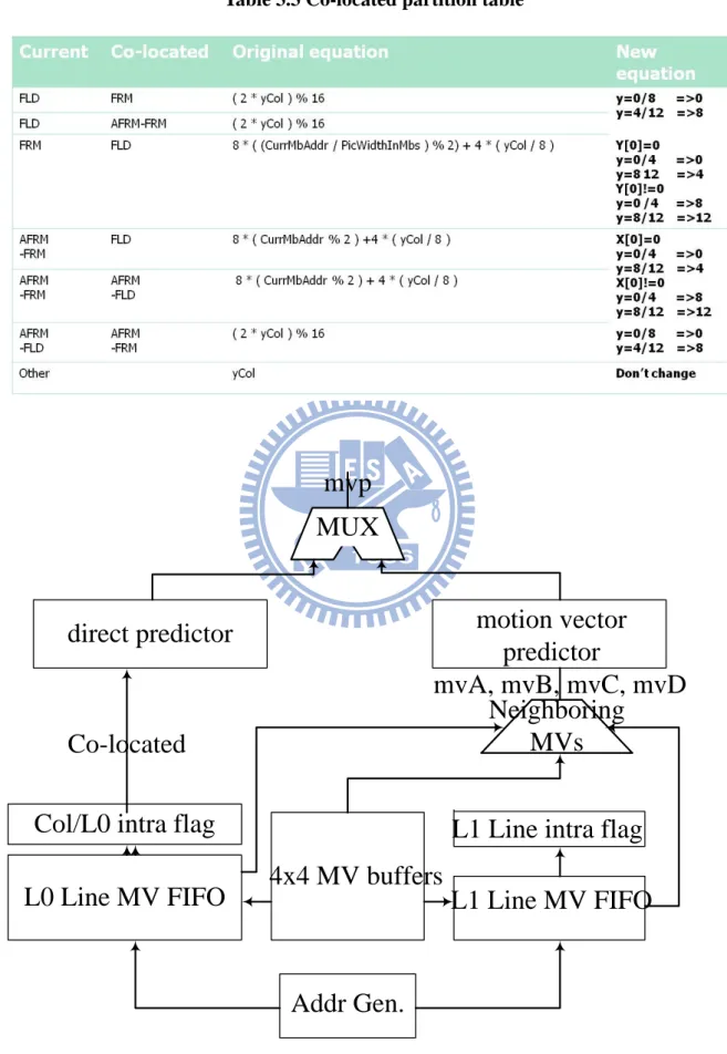
significantly reduce complexity. Table 3.2 shows the mapping table of co-located macroblock after coordinated method reduction. The Y means y-axis. Table 3.3 shows the mapping table
of co-located partition. Fig 3.5 shows the entire motion compensation architecture.
Table 3.2 Co-located macroblock table
Curr Col Original equation New equation
FLD FRM 2 * PicWidthInMbs * ( CurrMbAddr / PicWidthInMbs ) + ( CurrMbAddr
% PicWidthInMbs ) + PicWidthInMbs * ( yCol / 8 ) Y<<1+blk_Num[3] FLD AFRM
-FRM 2 * CurrMbAddr + ( yCol / 8 ) Y<<1+blk_Num[3] AFRM
-FLD 2 * CurrMbAddr + bottom_field_flag Y<<1+bottom_field_flag FRM FLD PicWidthInMbs * ( CurrMbAddr / ( 2 * PicWidthInMbs ) ) +
( CurrMbAddr % PicWidthInMbs ) Y>>1 AFRM FLD CurrMbAddr / 2 Y>>1 AFRM
-FRM AFRM-FLD 0 : 1 )2 * ( CurrMbAddr / 2 ) + ( ( topAbsDiffPOC < bottomAbsDiffPOC ) ? Y[0]=0 AFRM
-FLD AFRM-FRM 2 * ( CurrMbAddr / 2 ) + ( yCol / 8 ) Y[0]=0+blk_num[3] Other CurrMbAddr Don’t change
Table 3.3 Co-located partition table
L0 Line MV FIFO
Col/L0 intra flag
direct predictor
L1 Line intra flag
L1 Line MV FIFO
Addr Gen.
4x4 MV buffers
motion vector
predictor
MUX
mvA, mvB, mvC, mvD
Co-located
mvp
Neighboring
MVs
Fig 3.5 Motion vector generator architecture
3.3 Interpolator Design
3.3.1 Luma Interpolator Design
F
IR
F I R
F I R
F I R
Fig 3.6 Separate 1-D interpolator design (no parallel)
In this subsection, several different interpolator designs will be presented. Reviewing the fractional pixel interpolation for H.264/AVC in Fig 2.5, 6-tap FIR with (1, -5, 20, 20, -5, 1)
coefficient and bilinear filter are needed for half and quarter pixel interpolation. For cost and area efficiency consideration, Li‟s and Shen‟s interpolator filter unit and two-stage recursive
algorithm is proposed in [10] and [11]. These designs are area efficiency and suitable for P slice. However, as for B slice, throughput is a very important issue and long execution cycles
in these designs cause the real-time of video decoding cannot be meted.
Oppositely, consider throughput and standard-compatible design, Chien‟s [4] proposed
separate 1-D design that separates horizontal and vertical interpolation and processes in parallel based on 4 x 4 block size. This design owns better throughput, although it may need
more storages. Fig 3.6 shows separate 1-D interpolator design without processing in parallel.
Table 3.3 Comparison of execution cycles for different architectures
Architecture Ideal execution cycles
Shen’s and Li’s desing 13
Separate 1-D (no parallel) 36
Separate 1-D (2 parallel) 18
Separate 1-D (4 parallel) 9
Assuming that all 9 x 9 interpolated data for each 4 x 4 block are ready and they can be accessed randomly, Table 3.3 lists the execution cycles for different architecture. For Shen‟s
and Li‟s design, the result outputs depend on fractional pixel positions. For a, b, c, d, h, and n position 4 clock cycles are needed to finish one 4x4 block. For e, g, p, and r, it takes 8 cycles
to finish one 4 x 4 block interpolator. For f, j, q, i, and k, the cycles to finish one 4x4 block are 13 cycles which detailed operation is described in Li‟s [10] and Shen‟s [4]. As for separate
1-D design, the first data outputs at the 6th clock cycle and the following 3 data generates after 3 clock cycles. Therefore, the separate 1-D design without parallel needs 36 ((6 + 3) x 4)
cycles to complete interpolation of one 4 x 4 block. Similarly, separate 1-D design with 2 and 4 parallel requires 18 ((6 + 3) x 2) and 9 (6 + 3) cycles respectively. Finally, 4-parallel
separate 1-D architecture is our selection due to smaller required execution cycles that can be hidden below data-read cycles from frame memory.
a
c
G
h
d
n
H
m
M
s
N
f
e
g
j
i
k
q
p
r
b
Fig 3.7 Only one half pixel is needed
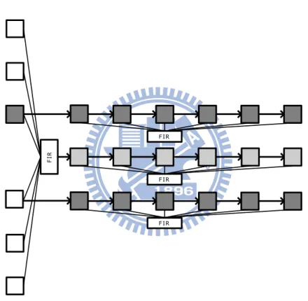
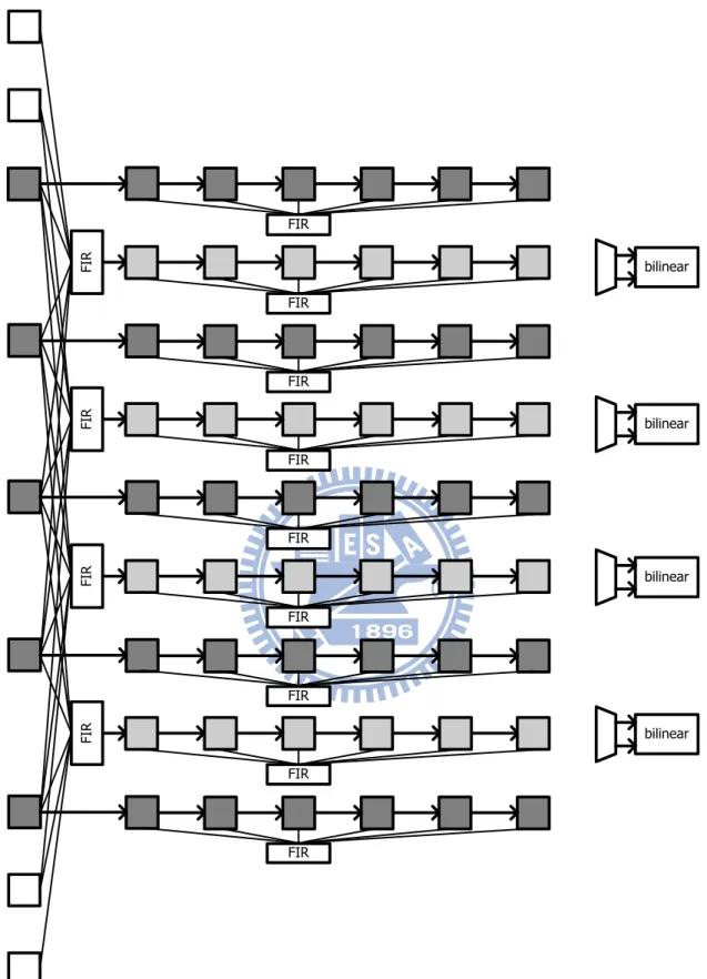
Fig 3.8 shows original 4-parallel separate 1-D luma interpolator. For cost consideration, multiplier in FIR can be simplified to adders and shifters. We will discuss FIR design later.
Because the original 4-parallel separate 1-D interpolator produces b and s half pixels at the same time for produce any position fractional pixel. However, either b or s half pixels is
needed when produce interpolated pixel. If we check MV, we can know which half is needed after all. Therefore, we can modify 4-parallel separate 1-D interpolator to reduce the path
storages and one FIR. The similar design can be seen in [12][13] and [14], but these designs require four multiplexers and we require only one multiplexer. Fig 3.9 shows the enhance
FI R FIR FIR FIR FIR FIR FI R FIR FI R FIR FIR FI R FIR bilinear bilinear bilinear bilinear
FI R FIR FIR FIR FIR FIR FI R FIR FI R FIR FI R FIR bilinear bilinear bilinear bilinear
3.3.2
Chroma Interpolator Design
A B D E G H C F I e h f gFig 3.10 Interpolation window for each 2 x 2 chroma block
] * * ) 8 [( * ] * * ) 8 [( * ) 8 ( * * * * ) 8 ( * ) 8 ( * * ) 8 ( * ) 8 ( D yFrac B yFrac xFrac C yFrac A yFrac xFrac D yFrac xFrac C yFrac xFrac B yFrac xFrac A yFrac xFrac i Eq. 3.1
Because of 4:2:0 chroma format and quarter precision of luma inter prediction, chroma inter prediction displacement can achieve one-eighth motion accuracy. Chroma inter
prediction must process based on 2 x 2 block size when luma inter prediction process based on 4 x 4 block size. Chroma interpolation requires 3 x 3 interpolated data for each 2 x 2 block
as shown in Fig 3.10. For chroma 2 x 2 block including A, B, C and D, the corresponding fractional sample is e, f, g and h whose precision is one-eighth. Compared with direct
mapping design with 8 multipliers which equation is listed in Fig 2.5 (c), we rewrite the equation listed in Eq. 3.1 and the number of multiplier number can be reduced to 4.
(8 ) * [ (8 ) * * ] * [ (8 ) * * ] (8 ) * * (8 - ) * * i x F r a c y F r a c A y F r a c C x F r a c y F r a c B y F r a c D F r a c M F r a c N M N F r a c O F r a c P Eq. 3.2
We can also rewrite the equation listed in Eq. 3.2. The Frac, O, and P are any corresponding value in Eq. 3.2. We can find as luma interpolator, chroma interpolator can
separate into horizontal and vertical filter. The corresponding separate 1-D design is illustrated in Fig 3.11 (a) and the vertical / horizontal filter is illustrated in Fig 3.11 (b).
2-parallel separate 1-D chroma interpolator are required to generate interpolated value in 2-pixel parallel, and it takes 3 cycles to filter 2 x 2 pixels if all required interpolated data are
ready and they can be accessed randomly. Based on 2-parallel separate 1-D chroma interpolator design illustrated in Fig 3.12, only one cycle latency is required.
yFrac xFrac round (b) (a) FI R FIR 8 Frac + * -*
Fig 3.11 (a) Chroma interpolator, (b) vertical/horizontal filter
A B D E G H C I F e h f g yFrac xFrac round FI R FIR yFrac xFrac round FI R FIR
Fig 3.12 2-parallel chroma interpolator
3.3.3
Combine Luma and Chroma FIR Design
<< 2 << 2 Luma Output Luma Output = A - 5B + 20C + 20D - 5E +F A F B E C D round (a) (b)
Fig 3.13 (a) Luma FIR design in Chen’s [3], (b) bilinear filter
Especially note that luma and chroma interpolation for H.264/AVC are different. That is,
no matter what on algorithm level or hardware level, the computation sources cannot be shared. Therefore, the combination of luma and chroma parts is the space of improvement. As
luma and chroma interpolator filter described in above, the adder and shifter can be shared when the architecture of chroma horizontal/vertical filter in Fig 3.11 (b) restructure to adder
and shifter. Besides, we can further reduce critical path by merge rounding stage. The combined interpolator design is shown in Fig 3.14 and the cost penalty is MUX x 2 and
bitwise AND x 6 when compared with the FIR design proposed in Chen‟s [3] and shown in Fig 3.13. Fig 3.15 illustrates the decoding path of luma FIR filter and chroma
horizontal/vertical filter. Because chroma interpolation for H.264/AVC is 2 x 2 block size basis, only eight luma FIR filters are required to replace with combined luma/chroma
interpolators. Fig 3.16 indicates the entire interpolator architecture for H.264/AVC.
<< 2 << 2 << 3 Chroma Output Bitwise AND Luma Output << 1 Rounding Coefficient
<< 2 << 1
<< 3
Chroma Output
XFrac[0]YiFrac[0]XFrac[1]YiFrac[1] XFrac[2]YiFrac[2]
Frac
Chroma Output =Frac*X + (8-Frac)*Y Y << 2 << 2 Luma Output A 1 F 1 B 1 E 1 C 1 D 1 Luma Output = (A - 5B + 20C + 20D - 5E +F +16 )>>5 (b) 16 >>5 0 (a)
R
_F
IR
FIR
FIR
FIR
FIR
R
_F
IR
R_FIR
R_FIR
R_FIR
Restructured interpolator design
R_FIR
R_FIR
R
_F
IR
R
_F
IR
Reuse for Cb
Reuse for Cr
3.3.4
Cost Analysis
Table 3.2 Comparison of requisite modules
Wang‟s [15] ISCAS‟05 Chen‟s [16] ICASSP‟06 Li‟s [10] ISCAS‟07 Tsai‟s[14] MWSCAS‟05 Shen‟s [11] ICME‟09 Proposed FIR 13 12 4 12 4 12 Bilinear 2 12 4 4 4 0 Technology (um) 0.18 0.18 0.18 0.18 0.18 0.09 Gate count 20,686 15,000 13,027 21,506 11,823 13,201 Working Frequency (MHz) 100 150 100 125 100 100 Latency (Cycles/MB) luma+chroma 560 320 304 144+NA 288+NA 144+48
Because of multipliers of 6-tap filter are simplified to adders and shifters in all references.
Therefore, in literature [10] and [11] use hardware sharing 6-tap FIRs to compute twice to reduce area cost in interpolator design. However, throughput is a very important issue and
long execution cycles in interpolator design lead to not enough throughput in B slice. Our restructured interpolator combines luma and chroma filter and through determine MV to
reduce a filter and one-path storages in traditional design. Table 3.2 lists the comparisons between our restructured interpolator design and other design. It shows our interpolator can
almost achieve as gate count of [10] and [11] and owns enough throughputs although it requires paying some control overhead to support multi-mode operations.
3.4 Weighted Prediction
lo g 0 1 0 1 ( ( 0 * 1 * 2 W D) ( lo g 1) ) ( ( 1) 1) p p L W p L W W D o o Eq. 3.3 lo g 1 0 0 lo g 1 1 1 { [ ( ( 0 * 2 ) lo g ) ] [ ( ( 1 * 2 ) lo g ) ] 1} 1) W D W D p p L W W D o p L W W D o Eq. 3.4 lo g 1 0 0 lo g 1 0 0 ( 0 * 2 ) lo g ) { 0 * [ 2 ( lo g ) ] } lo g W D W D p p L W W D o p p L W o W D W D Eq. 3.5Weighted prediction is the final stage of motion compensation behind the interpolator. Weighted prediction is a tool of scaling motion compensated samples to increase the video
quality in H.264/AVC video decoding. In this subsection, weighted predictor architecture is proposed to collocate with interpolator and eliminate the latency overhead. Chen‟s [16]
proposed weighted prediction architecture has low complexity. However, it has long critical path and large memory requirement (1.5kb). The design of Azevedo‟s [12] weighted predictor
is simply implemented by direct mapping design and require an embedded memory to store rounding coefficient. Compared with direct mapping design which equation is listed in Eq.
3.3, we can use the same predictor twice to generate predicted value, first is LIST_0 prediction and second is LIST_1 prediction as shown in Eq. 3.4. The component of rounding
and offset can be advanced and combined in the same stage. Therefore, the predictor can be further modified to reduce the critical path as shown in Eq. 3.5. Moreover from Eq. 3.5, the
W0 means weight factor and the value depend on weight flag from bit-stream. When weight
When weight flag is equal to 0, weight factor shall be in the range of 20 to 27, inclusive [1]. From the above discussion, if we determine the highest weight factor two bit we can use an
eight bits multiplier and shifter instead of a nine bits multiplier. The predictor is shown in Fig 3.17. M U X + offset <<7 * Weight factor[7:0] predPart LogWD + >> Round Weight factor[8:7] <<
Fig 3.17 Weighted predictor design
Moreover, when B slice is involved, we use hardware sharing to operate twice. In
addition, a 4 x 4 storages array is required to store intermediate results. Fig 3.18 illustrates the complete weighted predictor design. The same as temporal direct mode in motion vector
generator, weighted predictor has implicit mode which weighting factors are calculated based on the relative temporal positions of LIST_0 and LIST_1 reference picture. Weighting factor
in the implicit mode is derived from temporal direct mode data-path in order to reduce hardware cost. Furthermore, divider occupies the main area cost and computation time in the
dividend is a constant value. Table 3.2 lists the comparison for implementation results. For [12], it was not presented in comparison because lack of related detail information.
Predictor
1
Predictor
2
B-L1
M
U
X
P slice
C
lip
Luma/Cr
4x4
Buffer
Luma/Cb
A
v
er
ag
e
B-L0
Fig 3.18 Entire weight predictor architecture
ICASSP‟06[16] proposed
Multiplier (bits) 9 8
Technology .18um .90um
Gate count 12,960 6,412
Working frequency 87MHz 100MHz
3.5 Summary
In this chapter, a motion compensation engine for H.264/AVC Main/High Profile
decoder is presented. As for sharing design issue for multi-profile, our MVG use the same module and storages to deal with P slice and B slice which include MBAFF and non MBAFF.
Our restructured interpolator presents the area efficiently compared with traditional design and it is suitable for high throughput application such as coded in B slice video decoder.
Besides, the weighted predictor through hardware sharing with temporal direct mode and critical path shorten to achieve area efficiency. When weighted predictor collocates with
Chapter 4
Memory Bandwidth Reduction
4x4 output pixels
9x9 reference pixels
interp
olatio
n
Fig 4.1 4 x 4 block window and the corresponding 9 x 9 interpolation window
Considering luma interpolation, the half position samples interpolated by applying 6-tap
FIR filter and quarter position samples performed by applying using bilinear filter. It means interpolator needs six reference pixels to produce one interpolated pixel. Fig 4.1 shows to
interpolate each fractional sample value for each 4 x 4 block size; it needs 9 x 9 interpolation window. Chroma interpolation, of which concept is similar to luma, interpolates each
fractional sample value for each 2 x 2 block size, it needs 3 x 3 interpolation windows. When frame size is large and frame rate is high, interpolation causes heavy loading of memory
bandwidth. Moreover, motion compensation involves Main/High Profile; it supports B slices in which reference frame from one direction increase to two directions. From the above
interpolator needs memory bandwidth requirement, 398MB/s in P slices and 796MB/s in B slices, when support 1080 HD @ 30 fps. The heavy loading of memory bandwidth also means
huge power consumption for bus activity and data operation.
The rest of this chapter is organized as follows. Firstly, section 4.1 discusses our
reduction strategies of memory bandwidth. In addition, an analysis of bandwidth reduction limit is presented in section 4.2. Finally, summary is given in section 4.3.
4.1 Reduction strategies of memory bandwidth
Memory bandwidth always dominates the performance of entire video decoder. Several
methods have been proposed to reduce the required memory bandwidth and they can be mainly classified to two directions, first one is frame recompression and another one is
redundancy reduction of pixels transmission. With regard to the frame recompression, Fig 4.2 illustrates the concept. Frame data will be compressed before writing to frame memory, and
reference frame data will be decompressed before reading into video decoder. However, frame recompression method must consider many issues which like necessary random access
capability demanded from motion compensation, low complexity property due to area cost and power saving, and minimize required additional execution cycles to compress/decompress
data such that meet the real time throughput requirement of video decoder. Here we do not go into detail because our system have two dedicated modules, embedded compressor, between
motion compensation and frame memory and embedded decompressor between frame memory and de-blocking module respectively.
Video Decoder Frame Memory recompress decompress Global bus
As for second solution, transmission reduction of redundant pixels, which can be classified into two solutions that first one is data fetch time reducing and the other one is data
(pixel) reusing. The following subsection will discuss the detail of reduction strategies of memory bandwidth. Subsection 4.2.1 illustrates first strategy of data fetch times reducing.
Subsection 4.2.2 gives second strategy of data fetch times reducing. Subsection 4.2.3 illustrates first strategy of data reusing. Finally, subsection 4.2.4 presents second strategy of
data reusing.
4.1.1
Exact Fetch Necessary Pixels
a
c
G
h
d
n
H
m
M
s
N
f
e
g
j
i
k
q
p
r
b
Fig 4.3 Fractional sample positions for quarter sample luma interpolation
Fig 4.3 illustrates the luma samples „a‟ to „s‟ at fractional sample positions. In traditional
method, when interpolate fractional pixel, it always fetch 9x9 interpolation windows. However, there are not all pixels required in all fractional sample position. For example, the
sample at half sample position labeled b is derived by the nearest integer position samples in the horizontal direction. Similarly, the sample at half sample position labeled h is derived by
the nearest integer position samples in the vertical direction. Fig 4.4 illustrates interpolation of the samples at a, b, and c positions only need 9 x 4 interpolation windows. Fig 4.5 illustrates
interpolation of the samples at d, h, and n positions only need 4 x 9 interpolation windows. We can depend on motion vector value to exact fetch necessary pixels instead of fetch 9 x 9
interpolation window. Similar to luma interpolation, chroma interpolation can determine motion vector to decide interpolation window as well. Table 4.1 shows the summary of luma
interpolation windows. Table 4.2 shows the summary of chroma interpolation windows. The strategy is also used in other design [14], [10], and [11]. As for bandwidth reduction result, we
will show it later.
4x4 output pixels
9x4 reference pixels
interp
olatio
n
Fig 4.4 Fractional sample only need horizontal samples
. interp olatio n 4x9 reference pixels 4x4 output pixels
![Fig 2.3[8] shows the H.264/AVC profile on ARM processor. The reference software is JM 8.2 [7]](https://thumb-ap.123doks.com/thumbv2/9libinfo/8742359.204423/16.892.175.724.536.868/fig-shows-avc-profile-arm-processor-reference-software.webp)