Effective Learning Model and activate learning algorithm for improving learning efficiency

Effective Learning Model and Activate Learning Algorithm

for Improving Learning Efficiency

SHIH-JUNG PENG*_{, PI-FENG LIANG}* _{AND DENG-JYI CHEN} Institute of Computer Science and Information Engineering

National Chiao Tung University Hsinchu, 300 Taiwan

In recent years, technology developments are more rapidly. How to learn and obtain desired knowledge efficiently has become an important but complicated problem. We hope that there are methods can give us some suggestions about how to learn knowledge efficiently. In this paper, we introduced some learning behavior of people, and then use our designed Effective Learning Curve Model to imitate this learning phenomenon. Us-ing our learnUs-ing function model, we can imitate people’s learnUs-ing behavior through pre- testing. Every one has different learning behavior functions on learning distinct courses. Different learning sequence of courses will cause different learning efficiency. From this view, we proposed Max Learning Efficiency Slope First Algorithm (MLESFA) by dif-ferential learning functions to give people some suggestions about courses learning se-quence and obtain desired knowledge efficiently. These algorithms also can help us to understand how much time we have to spend on each course in order to get better learn-ing efficiency under time limitation. Finally, we make some learnlearn-ing example and com-pare simulation results with other courses learning algorithms. From the simulation re-sults, we can see that our MLESFA algorithm has better learning efficiency than others.

Keywords: e-learning, learning algorithm, learning function, learning model, learning

ef-ficiency, learning behavior

1. INTRODUCTION

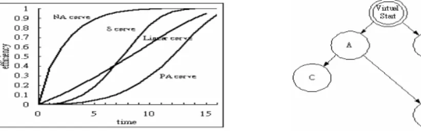
Technology developments are progressive rapidly in the world. The things people deal with have become more and more complex. Many ten years ago, for the research of building airplane, Wright [1] had used math methods to create learning curve function and develop first thesis about learning curve. From that time, learning methods have been discussed for distinct application plan and different models also had been produced. If we set horizontal axis indicates learning time period on courses, while the vertical axis indicates learning efficiency, we call this figure as learning curve. People’s learning curves are different and will be changed because of many reasons such as difficulty of works, learning motivation, knowledge background of learners, and some other reasons. There are some typical learning curves describe as follow, and shown in Fig. 1 (a). (a) Negative Accelerating Curve

Learning efficiency make a fast progress in the beginning, after that the learning

effi-Received August 31, 2005; revised January 18, 2006; accepted March 9, 2006. Communicated by Pau-Choo Chung.

* _{This research was supported in part by the National Science Council (Taiwan), Bestwise International} Com-puting Co., CAISER (National Chiao Tung University, Taiwan) and Ta Hwa Institute of Technology.

Shih-ciency will slow down gradually. Perhaps the contents are simple at the first and will be harder than before.

(b) Positive Accelerating Curve

Learning efficiency make a slow progress in the beginning, after that the learning ef-ficiency will be speeding gradually. Maybe, learner has been trained at the first time and will get some experience from that. Next time, they will spend less time and get better learning efficiency.

(c) S Accelerating Curve

Learning efficiency curve is the combination behavior of NA curve and PA curve. (d) Linear Accelerating Curve

The proportion of learning efficiency to spending learning time is linear equation. It can be written as η = a * t, where η: learning efficiency, a: constant parameter, t: spending time.

Fig. 1. (a) Typical learning curve. Fig. 1. (b) Courses learning sequence graph.

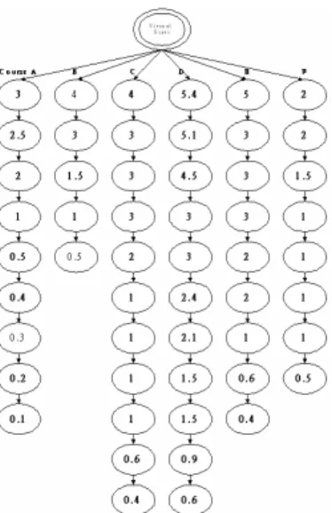
If there are some knowledge courses we prepare to learn, we can make their rela-tions into a learning graph as shown in Fig. 1 (b). In that, nodes represent learned courses and arrows mean courses learning sequence. For example, people do not allow learning course C till course A has been learned and passed, or the learning efficiency will de-crease, and we set this decreasing parameter ∂. Of course, there are some courses ing independent to others, such as course A and course B. That means we can start learn-ing from either course A or course B. For the reason, we use ‘virtual start node’ as the beginning of learning graph.

Under this course learning graph, we hope people can learn more efficiently with spending minimum learning time on each course. For this reason, we design new learn-ing function model to imitate people’s learnlearn-ing behavior. We also proposed Max Learn-ing Efficiency Slope First Algorithm (MLESFA) to improve group courses learnLearn-ing effi-ciency. At the end, we compare simulation results of our MLESFA algorithm with other algorithms. The simulation comparison is shown in Figs. 8 and 9. We can see that our algorithm has better simulation result and can improve learner’s group courses learning efficiency.

The remainder of this paper is organized as follows. In section 2, we introduce some related work and compare them with our proposed methods. In section 3, we proposed our learning function model to imitate people’s learning behavior. Learning efficiency algorithms are described in section 4. The simulation results and comparisons are pre-sented in section 5. Finally, we provide conclusion in section 6.

2. RELATED WORK

Learning curve can be described in math function for different learning characteris-tic. Five commonly used learning curves are described in Yelle [2], and are introduced as following:

(a) Log-linear model [1] f(x) = a1x-b

f(x): time needed for xth production a1: time needed for 1st production

b: learning coefficient, b = − (ln r/ln 2) r: learning rate

(b) Standford-B model [3] f(x) = a1(x + B)-b

B: constant, between 0 and 10 (c) De Jong Model [7]

f(x) = a1(M + (1 − M)x-b)

M: constant, between 0 and 1 (d) S Curve Model [4]

f(x) = a1(M + (1 − M)(x + B)-b)

(e) Time Constant Model [6] Y(t) = Yc + Yf (1 − e-t/τ₎

Yt: production numbers at time t

Yc: production numbers at time t = 0

Yf: adding production numbers through learning

τ : learning time constant

Learning model in Yelle [2] are suitable for special condition, but can not cover all learning behavior we have introduced before, and will be limited in some learning appli-cation area. In this paper, we designed Effective Learning Curve Model that can imitate most learning behavior of people by tuning function parameter. After that, we also pro-posed Max Learning Efficiency Slope First Algorithm (MLESFA) to improve people’s learning efficiency under learning group courses, and make some example to prove that our MLESFA algorithm has better learning efficiency.

3. HEURISTIC LEARNING MODEL

In this section, we try to find a learning equation which can imitate most of the learning behavior of people, as in Fig. 1 (a).

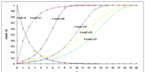
At first, we choose e-t as our base function: Where,

e-xt = 0, if t → ∞, e-xt _{= 1, if t → 0.}

Fig. 2. Exp( ) function under irregularly changing speed of the parameter x.

Function 1 − e-xt _{will become that,} 1 − e-xt _{= 0, if t → 0,}

1 − e-xt _{= 1, if t → ∞.}

We attempt to change parameter ‘x’ from 0 to ∞ including with irregular speed. Curve of function 1 − exp(− x) in Fig. 2 is under changing x from 0 to 10 stepped 0.5 regularly. In function 1 − exp(− x1), x1 changed from 0.05 to 10 under increasing irregu-lar speed 1.3. In the same way, x2 with speed 1.35, x3 with speed 1.5, x4 with speed 1.8 respectively.

Where,

Speed2 = Speed1 * 1.3,

Speedn = Speedn-1 * 1.3, Speedn = Speed1 * 1.3n-1.

From the results of the Fig. 2, we found that proposed learning function model could imitate the learning curves we have introduced in Fig. 1 (a) by tuned the combina-tion of parameters ‘a’, ‘b’, ‘c’. We proposed η(t) = c(1 − exp(− a(nt)b_{/(1 − nt))) as our} learning function model under experimentally testing. In that, t is time sequence, ‘a’ and ‘b’ are function parameter in order to imitate learner’s learning behavior, n is simulation time slot range, used to 0.01, ‘c’ is function coefficient indicating learning speed of imi-tated learning function.

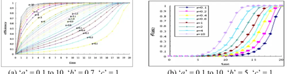
Using function f = η(t), and tuning the parameter ‘a’, ‘b’ and ‘c’, we can obtain some different learning curves, including Negative accelerating curves, Positive acceler-ating curves, S acceleracceler-ating curves and Linear acceleracceler-ating curves. In the following, we set parameter ‘a’ from 0.1 to 10, parameter ‘b’ from 0.7 to 5 and parameter ‘c’, the speed-ing coefficient of learnspeed-ing function, to 1. We can get relative function curves shown in Figs. 3 (a-b), and compare these figures, the effects of parameter ‘a’, ’b’ and ‘c’ on learn-ing function model are shown in Figs. 4 (a-c).

From Figs. 3 (a-b), if we want to make a imitation of learner’s learning curve, we can set the range of parameter ‘a’ between 0.1 to 10, parameter ‘b’ between 0.7 to 5 and ‘c’ = 1. If we want the imitation curves more precisely, we can just tune parameter ‘c’ from 0.8 to 2.0. From experiments, effects of parameter ‘a’ on learning function are shown in Fig. 4 (a), effects of parameter ‘b’ are in Fig. 4 (b), effects of parameter ‘c’ are shown in Fig. 4 (c), respectively. Therefore, we can emulate some different learning behavior

(a) ‘a’ = 0.1 to 10, ‘b’ = 0.7, ‘c’ = 1. (b) ‘a’ = 0.1 to 10, ‘b’ = 5, ‘c’ = 1. Fig. 3. Imitating learning curve under parameters ‘a’ = 0.1 to 10, ‘b’ = 0.7 to 5, ‘c’ = 1.

(a) Effects of parameter ‘a’. (b) Effects of parameter ‘b’. (c) Effects of parameter ‘c’. Fig. 4. Effects of parameters ‘a’, ‘b’ and ‘c’ on learning function.

(a) (b)

Fig. 5. Imitate learning function behavior curves under parameters ‘a’: 2~10, ‘b’: 1.5~5, ‘c’ = 1.

Table 1. Learning behavior imitation under combination of parameter ‘a’, ‘b’, ‘c’.

parameter NA Curve LA Curve PA Curve SA Curve

a 0.1 – 0.5 0.8 – 1.2 2.0 – 10 2.0 − 10

b 0.7 – 5.0 0.8 – 1.2 0.7 – 1.5 1.5 − 5

c 1 1 1 1

under combinations of parameter ‘a’, ‘b’ and ‘c’ between different range, as described in Table 1, and the imitating learning behavior curves are shown in Figs. 5 (a-b) .

But how can we get the parameter ‘a’, ‘b’ and ‘c’ of each user? For this purpose, we could use Item Response Theory (IRT) [12-14] which consider both course material dif-ficulty and learner ability. We also can collect and store much database about the rela-tions of learning efficiency with learner’s personality such as knowledge background, learning attitude, course difficulty, etc. Finally, we may use statistical application analy-sis method to find people’s suitable parameter ‘a’, ‘b’, ‘c’ and ‘n’.

Everyone has his own learning behavior curve in each course, and learning curve of each course would be different. Before start learning, we can make some pre-testing, using Item Response Theory, to predict suitable learning parameter ‘a’, ‘b’, ‘c’ and ‘n’ of each course respectively in order to get proper learning function to imitate learner’s learning behavior. Under group courses learning, there are some learning sequence rela-tions between courses. So, if we want to get the max learning efficiency in some condi-tion, the model can be formulated as follow.

Object to, 1 1 ( ) Max m n _i i ij i j d t W dt η = = ⎛ ⎞ ∗ ⎜ ⎟ ⎜ ⎟ ⎝

∑∑

ηi(t): learning function on course i

dηi(tij)/dt: learning efficiency of spending Δ time j on course i

Subject to, tij ≧ 0, T ≧ 0, 1 1 m n ij i j t T = = =

∑∑

∑

∑∑

In time tj, using differential method, we can choose max function slop 1 1 ( ) MAX(w d tj , dt η 2 2 ( ) ( ) , , ) j n j n d t d t w w dt dt η η

… as the first course learning priority.

4. ALGORITHM FOR IMPROVING LEARNING EFFICIENCY

In section 3, we introduced and compared some used learning functions, and pro-posed a new learning function model through Item Response Theory (IRT) [12-14]. We could use these learning functions to imitate learner’s learning behavior, to predict learner’s learning efficiency, and give some learning recommendation to the learners. But learner’s learning behaviors and learning function are not always fixed. Everyone could have different learning functions under distinct course, for example English and Math, environmental effect, pre-learning etc. One has one individual learning function under each course. Someone would have many learning functions, if there are numerous courses to be learned.

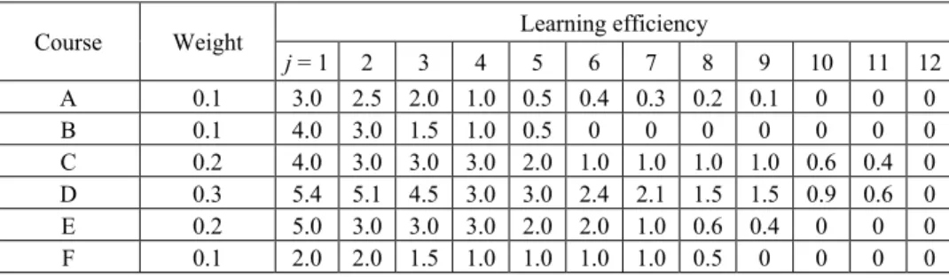
Table 2. Learning efficiency of each course under data sampling. Learning efficiency Course j = 1 2 3 4 5 6 7 8 9 10 11 12 A 30 25 20 10 5 4 3 2 1 0 0 0 B 40 30 15 10 5 0 0 0 0 0 0 0 C 20 15 15 15 10 5 5 5 5 3 2 0 D 18 17 15 10 10 8 7 5 5 3 2 0 E 25 15 15 15 10 10 5 3 2 0 0 0 F 20 20 15 10 10 10 10 5 0 0 0 0

Table 3. Learning efficiency*normalized weight of each course under data sampling.

Learning efficiency Course Weight j = 1 2 3 4 5 6 7 8 9 10 11 12 A 0.1 3.0 2.5 2.0 1.0 0.5 0.4 0.3 0.2 0.1 0 0 0 B 0.1 4.0 3.0 1.5 1.0 0.5 0 0 0 0 0 0 0 C 0.2 4.0 3.0 3.0 3.0 2.0 1.0 1.0 1.0 1.0 0.6 0.4 0 D 0.3 5.4 5.1 4.5 3.0 3.0 2.4 2.1 1.5 1.5 0.9 0.6 0 E 0.2 5.0 3.0 3.0 3.0 2.0 2.0 1.0 0.6 0.4 0 0 0 F 0.1 2.0 2.0 1.5 1.0 1.0 1.0 1.0 0.5 0 0 0 0

Table 4. Sorting courses learning efficiency by descending from Table 3.

Time tj j = 1 2 3 4 5 6 7 8 9 10 11 12 13 14 15 16 17 18 19 20 Learning sequence d1 d2 e1 d3 c1 b1 a1 b2 c2 c3 c4 d4 d5 e2 e3 e4 a2 d6 d7 a3 Each unit score 5.4 5.1 5.0 4.5 4.0 4.0 3.0 3.0 3.0 3.0 3.0 3.0 3.0 3.0 3.0 3.0 2.5 2.4 2.1 2.0 Total score 5.4 10.5 15.5 20 24 28 31 34 37 40 43 46 49 52 55 58 60.5 62.9 65 67 Time tj 21 22 23 24 25 26 27 28 29 30 31 32 33 34 35 36 37 38 39 40 Learning sequence c5 e5 e6 f1 f2 b3 d8 d9 f3 a4 b4 c6 c7 c8 c9 e7 f4 f5 f6 f7 Each unit score 2.0 2.0 2.0 2.0 2.0 1.5 1.5 1.5 1.5 1.0 1.0 1.0 1.0 1.0 1.0 1.0 1.0 1.0 1.0 1.0 Total score 69 71 73 75 77 78.5 80 81.5 83 84 85 86 87 88 89 90 91 92 93 94 Time tj 41 42 43 44 45 46 47 48 49 50 51 52 53 Learning sequence d10 c10 d11 e8 a5 b5 f8 a6 c11 e9 a7 a8 a9 Each unit score 0.9 0.6 0.6 0.6 0.5 0.5 0.5 0.4 0.4 0.4 0.3 0.2 0.1 Total score 94.9 95.5 96.1 96.7 97.2 97.7 98.2 98.6 99.0 99.4 99.7 99.9 100

In this section, our object is to provide a mathematical analysis in courses learning function and to define some learning behavioral strategies in order to obtain optimal courses learning sequence. And some examples will be briefly discussed. Now, we as-sumed there are six courses A, B, C, D, E, F and their weights of each course is normal-ized to be 1 / n . i i i W W =

∑

Where, W1 is signified as the weight of course A before normalizing. Let each

course weight equal to WA = 1, WB = 1, WC = 2, WD = 3, WE = 2, WF = 1. After

normaliz-ing, the weights of each course are become WnA = 0.1, WnB = 0.1, WnC = 0.2, WnD = 0.3, WnE = 0.2, WnF = 0.1. Using pre-testing, we can obtain user’s learning behavior curve of

each course and obtain discrete learning efficiency of each spending unit time by differ-ential course learning functions Dηi(t)|t=tj, as in Table 2. Multiplying value in Table 2 by

course weight Wi, we get the results in Table 3. Sorting learning efficiency field by

de-scending in Table 3, we could obtain value result as in Table 4.

Fig. 6. Sample learning efficiency under courses independence.

In the following discussion, first, we have made the assumption that courses are in-dependent to others, as shown in Fig. 6. In this condition, there are two questions we must face to solve. The first question is how can we know the minimum spending time on each course for the purpose of getting 60 score to pass the courseware, and the second question is how to obtain maximum course learning efficiency in order to get best score under given time limitation. For these reasons, we propose score base Algorithm 1.1 to solve first question, to know the minimum spending time on each course for the purpose of getting 60 score to pass all the courses, and time base Algorithm 1.2 to solve the sec-ond question, to get the best score under given time limitation.

Algorithm 1.1 Score base under courses independence

/* How much time we spend at least in order to obtain the score we wanted */ 1: make a pretest about learning courses in order to obtain learning behavior function 2: differential learning function dηi(tj)/dt, we can obtain the Δscore of spending time on

course learning, as in Table 2

3: multiplying obtained score in Table 2 by each course weight

4: sort the learning efficiency in Table 2 by descending, and shown the result in Table 3 5: input courses number cn and wanted score ws, where 60≦ws ≦100

6: initialize variable to zero 7: total score ts = 0

8: total learning time tlt = 0

9: course chapter learning sequence LS = ‘’ 10: for i = 1 to cn

11: time spending on each course chapter n(i) = 0 12: each course score obtained cs(i) = 0

13: next i

14: do while (ts < ws) 15: for i = 1 to cn

16: finding better course learning efficiency score bcs from ηi′⎢t=n(i)+1

17: next cn

/* from step 16, we could see that course j had better course learning efficiency and ob-tain score bcs, where j between 1 to cn */

18: n(j) = n(j) + 1 19: cs(j) = cs(j) + bcs 20: ts = ts + bcs

21: record chapter learning sequence to LS 22: end do

23: print the result ts, tlt, LS 24: for i = 1 to cn

25: print tsc(i), cs(i) 26: next i

27: end

Algorithm 1.2 Time base under courses independence

/* How many score we could obtain under learning time limited */ 1: to do the same steps 1 to 13 as in Algorithm 1.1

2: input time limited of learning courses tl 3: do while (tlt < tl)

4: for i = 1 to cn

5: finding better course learning efficiency score bcs from ηi′|t= n(i)+1

6: next cn

/* from step 5, we could see that course j had better course learning efficiency and obtain score bcs, where j between 1 to cn */

7: n(j) = n(j) + 1 8: cs(j) = cs(j) + bcs 9: ts = ts + bcs

10: record chapter learning sequence to LS 11: end do

12: print the result ts, tlt, LS 13: for i = 1 to cn

14: print tsc(i), cs(i) 15: next i

16: end

From the examples of courses independent learning graph as in Fig. 6, using Algo-rithm 1.1, if we want 60 score at least in order to pass the courseware, we must spend 17 unit times on courses. The time spending on each course is TA = 2, TB = 2, TC = 4, TD = 5, TE = 4, and TF = 0, and the final score we may obtain equal to ‘60.5’. Course learn-ing sequence suggestion is stored in variable LS = ‘d1 d2 e1 d3 c1 b1 a1 b2 c2 c3 c4 d4 d5 e2 e3 e4 a2’, as in Table 4. Under another time limitation condition, if we have 25 unit time, what score we can get max? Using time base Algorithm 1.2, we can get max final score equal to 77 and the time spending on each course is TA = 3, TB = 2, TC = 5, TD = 7, TE = 6, and TF = 2. Course learning sequence suggestion is LS = ‘d1 d2 e1 d3 c1 b1 a1 b2 c2 c3 c4 d4 d5 e2 e3 e4 a2 d6 d7 a3 c5 e5 e6 f1 f2’, as in Table 4.

Finally, we assume that some courses are dependent to others, as shown in Fig. 7. In Fig. 7, we also want to know the minimum spending time on each course for the purpose of getting 60 score to pass the courseware, and the maximum course learning efficiency in order to obtain best score under given time limitation. But some courses are dependent to each other, if course n − 1 has not passed, the learning efficiency of courses n will be influent. We raise parameter ∂ as this effect parameter, and learning efficiency will be changed to learning efficiency*(∂^m), in that 0≦∂ ≦1, m is the fail courses number before learned course n. As to these questions, we propose score base Algorithm 2.1 to solve first question, to know the minimum spending time on each course for the purpose of getting 60 score to pass all the courses, and time base Algorithm 2.2 to solve the sec-ond question, to get the best score under given time limitation. At first, we made a course learning choosing sequence principle, such that,

(a) high level learned course first,

(b) high course learning weight first with the same level, (c) effecting more learning courses first,

(d) learning from left to right.

Algorithm 2.1 Score base under courses dependence

1: make a pretest about learning courses in order to obtain learning behavior function 2: differential learning function, dηi(tj)/dt, we can obtain the Δscore of spending time on

course learning, as in Table 2

3: multiplying obtained score in Table 2 by each course weight

4: sort the learning efficiency in Table 2 by descending, and shown the result in Table 3 5: input courses number cn and wanted score ws, where 60 ≦ ws ≦ 100

6: initialize variable to zero 7: total score ts = 0

8: total learning time tlt = 0

9: course chapter learning sequence LS = ‘’ 10: for i = 1 to cn

11: time spending on each course chapter n(i) = 0 12: each course score obtained cs(i) = 0

13: using choosing principle for course learning, store course reading sequence into

crs(i) and course weight into cw(i)

14: next i 15: for i = 1 to cn

16: do while (cs(crs(i)) < ws * cw(crs(i)))

17: finding better course learning efficiency score bcs from ηi′|t=n(i)+1, as in Table 2

/* from step 17, we could see that chapter j of course crs(i) had better course learning efficiency and could obtain score bcs */

18: n(crs(i)) = n(crs(i)) + 1 19: cs(crs(i)) = cs(crs(i)) + bcs 20: ts = ts + bcs

21: record chapter learning sequence to LS 22: end do

23: next i

24: print the result ts, tlt, LS 25: for i = 1 to cn

26: print tsc(i), cs(i), crs(i), cw(i) 27: next i

28: end

Algorithm 2.2 Time base under courses dependence

1: to do the same steps 1 to 14 as in Algorithm 2.1 2: input time limited of learning courses tl 3: for i = 1 to cn

4: do while (cs(crs(i)) < 60 * cw(crs(i)) and tlt < tl)

5: finding better course learning efficiency score bcs from ηi′⎢t=n(i)+1, as in Table 2

/* from step 5, we could see that chapter j of course crs(i) had better course learning effi-ciency and could obtain score bcs */

6: n(crs(i)) = n(crs(i)) + 1 7: cs(crs(i)) = cs(crs(i)) + bcs 8: ts = ts + bcs

9: record chapter learning sequence to LS 10: end do

11: next i

12: to do the same steps 3 to 11 as in Algorithm 1.2 13: print the result ts, tlt, LS

14: for i = 1 to cn 15: print tsc(i), cs(i) 16: next i

17: end

From the course learning graph as in Fig. 7, using Algorithms 2.1 and 2.2, we can get course learning sequence such as course C, A, E, B, F, and D. If we want to pass all courses, the time we must spend on each course is TA = 3, TB = 2, TC = 4, TD = 4, TE = 4, TF = 4 and the score of each course we will get is as follow, SA = 75, score of course A, SB = 70, SC = 65, SD = 60, SE = 70, SF = 65, respectively. Therefore if we want to pass all the courses, we must spend at least to 3 + 2 + 4 + 4 + 4 + 4 = 21 unit times, and will obtain final score equal to (75 * 1 + 70 * 1 + 65 * 2 + 60 * 3 + 70 * 2 + 65 * 1)/10 = 66 with multiplying each course score and course weighting.

Another question, if we have unit time > 21, for example 30, what score we can get max? First, we use Algorithm 2.1 to make all courses pass, and then use Algorithm 1.2 to sort and get all the other course contains that we will spend learning times on it. Finally, following these steps, we can obtain the time we spend on each course, TA = 3, TB = 3, TC = 5, TD = 9, TE = 6, TF = 4 and get related scores as follow, SA = 75, SB = 85, SC = 75, SD = 95, SE = 90, SF = 65. At last, we obtain final score equal to (75 * 1 + 85 * 1 + 75 * 2 + 95 * 3 + 90 * 2 + 65 * 1)/10 = 84. And the course learning sequence suggestion is stored in variable LS.

5. EFFICIENCY COMPARISON

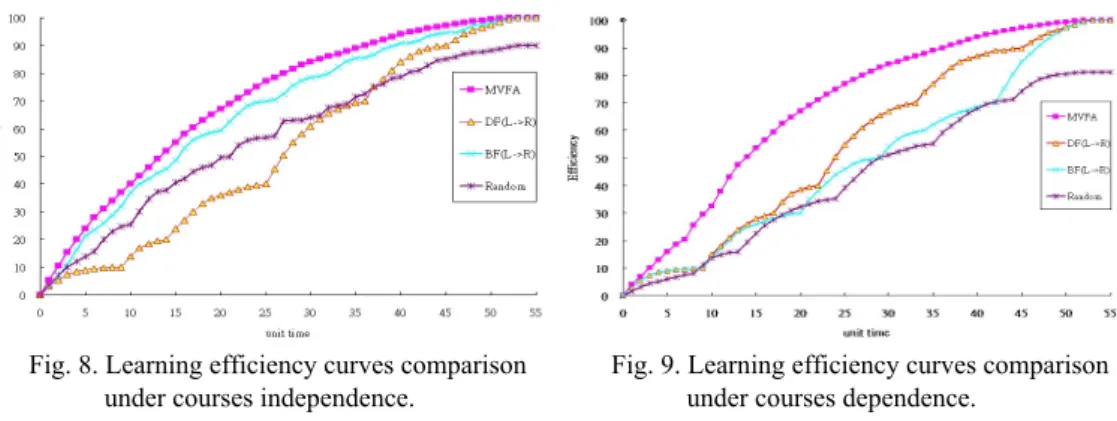
To prove our learning behavior function and learning algorithms having better learning efficiency, we use learning graph, Figs. 6 and 7 as our comparison example. Table 2 is learner’s learning efficiency of each course by differential course learning function and data sampling. At the first, we take Fig. 6 into consideration that courses are independent, and we compare MLESFA1 simulation result with course Depth First Al-gorithm (DFA), course Bread First AlAl-gorithm (BFA) and course Random AlAl-gorithm (RA). DFA learns all chapters of course A by sequence, after learned completely, next to learn course B, C, D, E and F. BFA learns chapter 1of course A at the first, next to chapter 1 of course B, C, D, E, and F, after that, learns chapter 2 of course A, B, C, D, E, F and will not stop till all chapters have been learned completely. RA means random choosing course chapter to learn. Because of course chapter having its learning sequence, random choosing course chapter to learn will affect chapter learning efficiency, we assume effect parameter η = ‘0.8’. The comparison learning efficiency curves are shown in Fig. 8 un-der course learning graph Fig. 6.

Fig. 8. Learning efficiency curves comparison under courses independence.

Fig. 9. Learning efficiency curves comparison under courses dependence.

learning sequence of our algorithm MLESFA by choosing course learning sequence prin-ciple are course A, C, B, E, F, D, courses learning sequence by algorithm DFA are course A, E, B, D, C, F, courses learning sequence by algorithm BFA are course A, C, E, B, F, D respectively. As to algorithm RA, we get randomly courses learning sequence, at here we supposed its course learning sequence are course F, B, D, C, E, A. Because courses are dependent, if parent courses haven’t passed yet, and we insist on learning following courses, the course learning efficiency will be influenced. This effect will bigger than courses dependent and we assumed this effect parameter η = 0.8. If learning course have m parent courses not passed, the influence will be changed to η^m. The comparison learning efficiency curves are shown in Fig. 9 under condition Fig. 7.

From above discussions, we can see that our algorithms has better learning effi-ciency result both in Fig. 8 under Fig. 6 courses independence, and in Fig. 9 under Fig. 7 courses dependence.

6. CONCLUSION

In this paper, we have made some contributions, (1) we proposed new effective heu-ristic learning function η(t) = c(1 − exp(− a(nt)b_{/(1 − nt))) to imitate people’s learning}

behavior. From tuning parameter ‘a’, ’b’, ‘c’ and ‘n’, we can imitate most people’s ing behavior including Negative accelerating learning curve, Positive accelerating ing curve, S accelerating learning curve and ‘linear’ accelerating learning curve on learn-ing courses or works. (2) Under time limitation, every one wants to understand how to learn will get the best result and how much time they have to spend on each course. Us-ing effective heuristic learnUs-ing function, we raised two different course learnUs-ing algo-rithm, score-based algorithm and time-based algorithm under the conditions of courses dependent and independent separately.

For getting better learning efficiency, we follow the steps:

Step 1: Obtain the learner’s learning function under pre-testing and (IRT).

Step 2: Sample learning efficiency of each course.

Step 3: Multiply learning efficiency by normalized weight of each course.

Step 5: Choose a suitable Algorithms 1.1, 1.2, 2.1 or 2.2 in section 4.

Through proposed algorithm simulation results, we could get suggestions about the course learning sequence, and the times we spend on each course in order to get better learning efficiency under time limitation. From the result comparison in Figs. 8 and 9, we could see that our proposed algorithm has better learning efficiency than others.

REFERENCES

1. P. T. Wright, “Factors affecting the cost of airplanes,” Journal of Aeronautical

Sci-ences, Vol. 3, 1936, pp. 122-128.

2. L. E. Yelle, “The learning curve: history review and comprehensive survey,”

Deci-sion Sciences, Vol. 10, 1979, pp. 302-328.

3. A. Garg and P. Milliman, “The aircraft progress curve modified for design changes,”

Journal of Industry Engineering, Vol. 12, 1961, pp. 23-27.

4. R. Cooper and R. S. Kaplan, “Activity-based systems: measuring the cost of re-source usage,” Accounting Horizon, Vol. 6, 1992, pp. 1-13.

5. V. Carchiolo, A. Longheu, and M. Malgeri, “Learning through ad-hoc formative paths,” in Proceedings of IEEE International Conference on Advanced Learning

Technologies, 2001, pp. 96-99.

6. F. W. Bevis and D. R. Towill, “Managerial control systems based on learning curve model,” Journal Production Resource, Vol. 11, 1972, pp. 219-238.

7. D. Jr. Jong, “The effects of increasing skill on cycle time and its consequences for time standards,” Ergonomics, Vol. 1, 1957, pp. 31-35.

8. W. H. Huang and M. S. Hacid, “Contextual knowledge representation, retrieval and interpretation in multimedia e-learning,” in Proceedings of the 4th IEEE

Interna-tional Conference on Information Reuse and Integration, 2003, pp. 27-29.

9. Y. J. Niganad and M. Bonney, “A comparative study of learning curves with forget-ting,” Applied Mathematical Modeling, Vol. 21, 1997, pp. 523-531.

10. R. A. Lawson, “Activity-based costing systems for hospital management,” CMA

Magazine, Vol. 68, 1994, pp. 31-35.

11. H. N. Lin, “An adaptive learning environment: a case study on high school mathe-matics,” Master’s Thesis, Department of Computer and Information Science, Na-tional Chiao Tung University, Hsinchu, Taiwan, 2001.

12. F. B. Baker, “The basics of item response theory. ERIC clearing house on assess-ment and evaluation,” University of Maryland, College Park, MD, http://ericae.net/ irt/baker, 2001.

13. F. B. Baker, Item Response Theory: Parameter Estimation Techniques, Marcel Dek-ker, New York, 1992.

14. R. K. Hambelton, H. Swaminathan, and H. J. Rogers, Fundamentals of Item Response

Shih-Jung Peng (彭士榮) received the B.S. degree in Electronic Engineering from the National Taiwan University of Science and Technology, Taipei, Taiwan, and M.S. degree in Computer Science and Information Engineering from National Central University, Taoyuan, Taiwan, in 1990 and 1994, respec- tively. He is now a Ph.D. student at Computer Science and Infor- mation Engineering Department of National Chiao Tung Univer- sity, Hsinchu, Taiwan, and he is also a Teacher at Computer and Communication Engineering of Ta Hwa Institute of Technology (THIT), Hsinchu, Taiwan. His research interests include e-learning, window’s application, performance and reliability modeling.

Pi-Feng Liang (梁碧峰) received a B.S. degree from the Department of Mathematics at National Tsing Hua University, and an M.S. degree from the Department of Computer Science and Information Engineering at National Taiwan University. He is currently a Ph.D. student in the Department of Computer Science and Information Engineering at National Chiao Tung University. He is now a Teacher in the Department of Information Management at Ta Hwa Institute of Technology (THIT), Hsin- chu. His research interests include e-learning, data mining and distributed systems.

Deng-Jyi Chen (陳登吉) received the B.S. degree in Com-puter Science from Missouri State University (cape Girardeau), U.S.A., and M.S. and Ph.D. degrees in Computer Science from the University of Texas, Arlington, U.S.A. in 1983, 1985, 1988, respectively. He is now a professor at Computer Science and In-formation Engineering Department of National Chiao Tung Uni-versity, Hsinchu, Taiwan. Prior to joining the faculty of National Chiao Tung University, he was with National Cheng Kung Uni-versity, Tainan, Taiwan. So far, he has been publishing more than 130 referred papers in the area of software engineering (software reuse, object-oriented systems, visual requirement representation), multimedia applica-tion systems (visual authoring tools), e-learning and e-testing system, performance and reliability modeling and evaluation of distributed systems, computer networks. Some of his research results have been technology transferred to industrial sectors and used in product design. So far, he has been a chief project leader of more than 10 commercial products. Some of these products are widely used around the world. He has been re-ceived both research awards and teaching awards from various organizations in Taiwan and serves as a committee member in several academic and industrial organizations.