依據製程能力指標Spk應用複式抽樣方法於供應商選擇

國立交通大學

工業工程與管理學系

碩士論文

依據製程能力指標

S

_pk

應用複式抽樣方法於

供應商選擇

Bootstrap Approach for Supplier Selection Based on

Process Capability Index

S

pk

研 究 生：褚耀聰

指導教授：彭文理

博士

吳建瑋

博士

依據製程能力指標

S

_pk

應用複式抽樣方法於

供應商選擇

Bootstrap Approach for Supplier Selection Based on

Process Capability Index

S

_pk

研 究 生：褚耀聰 Student : Yao-Tsung Chu

指導教授：彭文理 博士 Advisor : Dr. W. L. Pearn 吳建瑋 博士 Dr. Chien-Wei Wu

國 立 交 通 大 學

工 業 工 程 與 管 理 學 系

碩 士 論 文

A Thesis

Submitted to Department of Industrial Engineering and Management

College of Management

National Chiao Tung University

in partial Fulfillment of the Requirements

for the Degree of

Master

in

Industrial Engineering

May 2007

Hsinchu, Taiwan, Republic of China

依據製程能力指標

S

_pk

應用複式抽樣方法於

供應商選擇

研究生：褚耀聰

指導教授：彭文理 博士

吳建瑋 博士

國立交通大學工業工程與管理學系碩士班

摘要

現今的製造業裡，許多公司藉由增加外購的比重以維持自己的核心競爭力， 於是，供應商的選擇成為生產管理上重要的議題。在製造業裡，產品的良率一直 是判斷製程好壞的重要因素，Boyles 提出了一個和良率有一對一對應關係的製程 能力指標S_pk，過去有許多關於Spk指標的近似分配、估計和檢定，這些結果已被 應用在選擇單一供應商的研究，然而利用S_pk指標來同時檢定兩家不同供應商的議 題至今尚無人研究。這篇研究的主要目的就是在兩家相互競爭的供應商中，挑選 出一家具有較好製程能力的供應商，並建立一個依據S_pk指標選擇供應商的決策程 序。在本篇論文中，我們將利用複式抽樣法來建構兩個供應商間製程能力差異的 信賴下界，針對四個不同複式抽樣法來比較彼此之間犯錯機率及檢定力的表現， 為了實務應用上方便，我們建立一個在犯錯機率為 0.05 下，針對給定不同選擇能 力所需要的樣本數表格，最後我們也將研究的結果，應用在選擇兩家不同的彩色 濾光片廠商。 關鍵字：複式抽樣法、信賴下界、製程良率、供應商選擇。

Bootstrap Approach for Supplier Selection Based

on Process Capability Index

S

_pk

Student: Yao-Tsung Chu

Advisor：

.

Dr. W. L. Pearn

Dr. Chien-Wei Wu

Department of Industrial Engineering and Management

National Chiao Tung University

Abstract

In today’s manufacturing environment, many companies increase their out-sourcing level to keep their core competition. Supplier selection problems have become an important component of production management. Process yield is a standard criterion in the manufacturing industry as a common measure on process performance. Boyles proposed a index S_pk which provides an exact measure on

the process yield for normal processes. Many studies considered the assessment of index Spk for a single supplier. However, the testing procedure for two different suppliers selection based on S_pk has not been done today. The principal purpose of

this research is to determine the more capable process between two competing suppliers and provide a supplier selection procedure based on Spk. In this thesis, we implemented the bootstrap method to construct the lower confidence bound for the capability difference and the capability ratio between two given suppliers. The performance comparisons are made among the four bootstrap methods (the standard bootstrap (SB), the percentile bootstrap (PB), the biased corrected percentile bootstrap (BCPB), and the bootstrap-t (BT)) in terms of error probability and selection power. For convenience of applications, we tabulated the sample sizes required for various designated selection power. A real world case on the color filter manufacturing process is investigated to demonstrate the applicability of the proposed method in the end.

Key words: Bootstrap method, Lower confidence bound, Process yield, Supplier selection.

誌謝

這輩子寫過最完整且最令自己驕傲的一篇文章，就是這篇論文研

究，能夠完成這篇論文首先要感謝彭文理老師和吳建瑋老師，從彭老

師身上不僅學習到學術上的嚴謹態度，同時也學到了未來工作就業的

態度；感謝吳老師不定時的與我們討論研究上的作法，幫助我們更了

解論文內研究方法的意義。此外也非常感謝鍾淑馨老師在口試上給我

的寶貴意見，由於這些老師的幫忙，才讓這篇論文得以完成。

博班的學長姐們、MB517、MB519 的同學們，感謝你們讓我在研究

所的這兩年過的多彩多姿，尤其感謝我的兩個好戰友阿亮和龜苓膏，

有你們的幫忙，才可以讓我在回國最後口試階段順利進行，MB516 的學

弟妹們，感謝你們在我口試的時候幫忙準備老師們的點心，還有我大

學時期的好朋友 sath 讓我不用在回新竹的時候露宿街頭。

不免俗的要感謝我的父母，有你們的幫助，我才可以在無經濟壓

力下完成這個學位，最後把這篇論文獻給我的爺爺、奶奶，希望你們

看的到，知道我畢業了！

Contents

Abstract (Chinese)

... i

Abstract

... ii

誌謝

... iii

Contents

... iv

List of Table

... v

List of Figure

... vi

Notations

... x

1. Introduction

... 1

2. Literature Review

... 2

2.1 Process Capability Indices ... 2

2.2 Process Yield Based on Spk ... 3

2.2.1 ProcessYield ………..3

2.2.2 Yield Assurance Based on Spk………..3

2.3 Supplier Selection Problems based on PCIs... 4

3. Selection Method

... 6

3.1 Selecting a Better Supplier by Comparing Two Spk ... 6

3.2 Bootstrap Methodology... 8

4. Performance Comparison of Four Bootstrap Methods

... 12

4.1 Simulation Layout Setting ... 12

4.2 Error Probability Analysis ... 14

4.3 Selection Power Analysis ... 17

5. Supplier Selection Based on BCPB Method

... 19

5.1 Sample Size Determination with Designated Selection Power ... 19

5.2 Selecting the Better Supplier ... 23

6. Application Example:Color Filter Supplier Selection ...

24

6.1 Data Analysis and Supplier Selection... 25

7. Conclusions

... 27

List of Table

Table 1. Some Spk values and the corresponding values of fraction yield and nonconformities (ppm) ... 4 Table 2. Ca values and ranges of ... 12 Table 3. The parameter setting values for two manufacturing suppliers used in the

simulation study under Spk1Spk2 1.00………14

Table 4. The results of error probability analysis for difference test ... 16 Table 5. The results of error probability analysis for ratio test ... 16 Table 6. Simulation results of the four bootstraps methods for the difference and

ratio statistics... 17 Table 7. Sample size required of BCPB method for the difference statistics under

0.05

 , with power = 0.90, 0.95, 0.975, 0.99, Spk11.00,

2 1.10(0.05)1.50

pk

S  ... 19

Table 8. Sample size required of BCPB method for the ratio statistics under=0.05, with power = 0.90, 0.95, 0.975, 0.99, Spk11.00,

2 1.10(0.05)1.50

pk

S  . ... 20

Table 9. Sample size required of BCPB method for the difference statistics under 0.05

 , with power = 0.90, 0.95, 0.975, 0.99, Spk11.30,

2 1.40(0.05)1.80

pk

S  ... 20

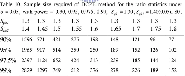
Table 10. Sample size required of BCPB method for the ratio statistics under 0.05

 , with power = 0.90, 0.95, 0.975, 0.99, Spk11.30,

2 1.40(0.05)1.80

pk

S  ... 20

Table 11. The calculated sample statistics for two suppliers ... 25 Table 12. The error probability of four bootstrap methods for the difference and

ratio statistics with 16 combinations of ( Cp1, Ca1) and ( Cp2, Ca2) under

1 2 1.00

pk pk

S S  ... 30 Table 13. Selection power of the four bootstrap methods for difference statistic with

sample size n = 30(10)200 ... 34 Table 14. Selection power of the four bootstrap methods for ratio statistic with

sample size n = 30(10)200 ... 37 Table 15. The sample data for supplier I ... 45 Table 16. The sample data for supplier II………...….45

List of Figure

Figure 1. Four processes with S_pk=1.00 ... 13

Figure 2. Error probability of four bootstraps under Spk1 Spk2 1.00 ... 15

Figure 3. Error probability of four bootstraps under S_pk2/S_pk11.00... 15

Figure 4. The selection power of the four Bootstrap methods for the difference statistic with sample size n=30(10)200. ... 18

Figure 5. The selection power of the four Bootstrap methods for the ratio statistic with sample size n= 30(10)200 ... 18

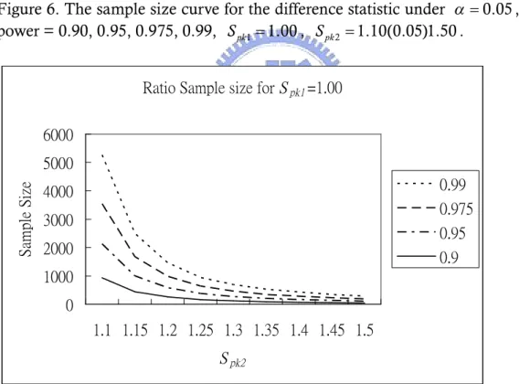
Figure 6. The sample size curve for the difference statistic under 0.05, with power = 0.90, 0.95, 0.975, 0.99, S_pk11.00, S_pk2 1.10(0.05)1.50…….21

Figure 7. The sample size curve for the ratio statistic under 0.05, with power = 0.90, 0.95, 0.975, 0.99, Spk11.00, ... 21

Figure 8. The sample size curve for the difference statistic under 0.05, with power = 0.90, 0.95, 0.975, 0.99, S_pk11.30, S_pk2 1.40(0.05)1.80... 22

Figure 9. The sample size curve for the ratio statistic under 0.05, with power = 0.90, 0.95, 0.975, 0.99, S_pk11.30,S_pk2 1.40(0.05)1.80 ... 22

Figure 10. The combination of TFT-LCD structure... 24

Figure 11. Histogram of data S1……….………..25

Figure 12. Histogram of data S2 ... 25

Figure 13. The difference statistic with sample size n = 30(10)200, 1 1.00 pk S  ,S_pk2 1.05 ... 40

Figure 14. The ratio statistic with sample size n = 30(10)200, S_pk11.00, 2 1.05 pk S  ... 40

Figure 15. The difference statistic with sample size n = 30(10)200, 1 1.00 pk S  ,S_pk2 1.10 ... 40

Figure 16. The ratio statistic with sample size n = 30(10)200, S_pk11.00, 2 1.10 pk S  ... 40

Figure 17. The difference statistic with sample size n = 30(10)200, 1 1.00 pk S  ,S_pk2 1.15 ... 41

Figure 18. The ratio statistic with sample size n = 30(10)200, Spk11.00, 2 1.15 pk S  ... 41

Figure 19. The difference statistic with sample size n = 30(10)200, 1 1.00 pk S  ,S_pk2 1.20 ... 41

Figure 20. The ratio statistic with sample size n = 30(10)200, Spk11.00,

2 1.20

pk

S  ... 41

Figure 21. The difference statistic with sample size n = 30(10)200,

1 1.00

pk

S  ,S_pk2 1.25 ... 42 Figure 22. The ratio statistic with sample size n = 30(10)200, Spk11.00,

2 1.25

pk

S  ... 42

Figure 23. The difference statistic with sample size n = 30(10)200,

1 1.00

pk

S  ,S_pk2 1.30 ... 42 Figure 24. The ratio statistic with sample size n = 30(10)200, Spk11.00,

2 1.30

pk

S  ... 42

Figure 25. The difference statistic with sample size n = 30(10)200,

1 1.00

pk

S  ,S_pk2 1.35 ... 43 Figure 26. The ratio statistic with sample size n = 30(10)200, Spk11.00,

2 1.35

pk

S  ... 43

Figure 27. The difference statistic with sample size n = 30(10)200,

1 1.00

pk

S  ,S_pk2 1.40 ... 43 Figure 28. The ratio statistic with sample size n = 30(10)200, Spk11.00,

2 1.40

pk

S  ... 43

Figure 29. The difference statistic with sample size n = 30(10)200,

1 1.00

pk

S  ,S_pk2 1.45 ... 44 Figure 30. The ratio statistic with sample size n = 30(10)200, Spk11.00,

2 1.45

pk

S  ... 44

Figure 31. The difference statistic with sample size n = 30(10)200,

1 1.00

pk

S  ,S_pk2 1.50 ... 44 Figure 32. The ratio statistic with sample size n = 30(10)200, Spk11.00,

2 1.50

pk

Notations

T ：target value

USL ：the upper specification limits presented by the process engineers LSL ：the lower specification limits presented by the process engineers m ：the midpoint between the upper and lower specification limits d ：the half specification width

 ：the population mean

 ：the population standard deviation

2

 ：the population variation

n ：the number of the sample size drawn from supplier B ：the number of bootstrap resamples

N ：simulation replicated times

* 1 pk S  ：the Spk1 

of bootstrap resamples from supplier I

* 2 pk S  ：the Spk2 

of bootstrap resamples from supplier II  ：the difference or the ratio of two suppliers’S_pk index

 ：the estimator of 

*

 ：the associated ordered bootstrap estimate of 

*

 ：the sample average of the B bootstrap estimates

*

1.

Introduction

Currently, many manufacturing industries have increased their out-sourcing level to keep their core competition. That is, they purchase various portions of components or subassemblies for their final products. In order to know if the supplier is qualified, some indices are needed. Process yield has long been one of the most standard criterion used in the manufacturing industry as a common measure on process performance. Process yield is defined as the percentage of processed product passing inspection. That is, the product characteristic must fall

within the manufacturing tolerance. When product units rejected

(non-conformities), additional costs would be incurred to the factory for scrapping or repairing the product. All passed product units are equally accepted by the producer, which incurs the factory no additional cost. On the other hand, consumer can save a lot of money from accepting producer, which has high level quality yield. In today’s high-tech industry, traditional sampling method is not enough because of the high level quality yield. Process capability indices (PCIs) have been widely used in the manufacturing industry and provided numerical measures on process performance. We can determine whether a production process is capable and infer the process yield based on PCIs. This fact brings the issue of supplier selection based on PCIs into the main focus.

Many individuals have indicated various approaches for supplier selection or process comparison problems based on PCIs. Most of these researches focus on single supplier selection before. They consider the assessment of capability for a single process. However, there are fewer studies investigate the testing procedure for two different suppliers selection. Discussion relative to the subject based on the index S_pk has not been concentrated. The principal purpose of this research is to determine the more capable process between two competing suppliers and provide a supplier selection procedure based on Spk.

In this thesis, we introduced process capability indices in common used, and reviewed some references about supplier selection problems based on PCIs first. Section 3 proposed to select a better supplier by comparing two Spk . We formulated the hypothesis testing and introduced the bootstrap methodology. In section 4, we analyzed the error probability and selection power by comparing four different bootstrap methods. For convenience of applications, we tabulated the sample sizes required for various designated selection power in section 5. At last, we demonstrated a real world case on color filter manufacturing process, and made a conclusion in section 6 and 7.

2.

Literature Review

2.1 Process Capability Indices

There are many capability indices proposed to use for evaluating a supplier’s process capability. The first process capability index in the literature was Cp. It was introduced by Juran et al. (1974), but did not gain considerable acceptance until the early 1980s. It is defined as:

 6

LSL USL

C_p   ,

where USL is the upper specification limit, LSLis the lower specification limit,

and  is the process standard deviation. The index measures capability in terms of process variation only and did not take process location into consideration. Pearn et al. (1998) introduced an accuracy index Ca to measure the magnitude of process centering. It is defined as:

| | 1 a m C d    ,

where  is the process mean, m



USLLSL



2, and d



USLLSL



2. The index Ca measures the centering tendency. User can get alerts from it if the process mean is deviate form the midpoint. Kane (1986) proposed the capability index Cpk, considered process location of mean and process variation. The index

pk

C determines process ability of reproducing items within the specified

manufacturing tolerance. It is defined as:









| | min , =min , 3 3 3 pk pu pl USL LSL d m C  C C _ _   _ .

Based on the expression of process yield, Boyles (1994) considered the yield index pk

S for normal process, as defined in the following:

1 1 1 1 { ( ) ( )} 3 2 2 pk USL LSL S             ,

where  is the cumulative density function (c.d.f) of the standard normal distribution N(0,1) . Hsiang and Taguchi (1985) introduced the index Cpm , independently proposed by Chan et al. (1988). The index Cpm focuses on the product loss when one of its characteristics departs from the target value T. It is defined as: 2 2 6 ( ) pm USL LSL C T       .

2.2 Process Yield Based on Spk

2.2.1 Process Yield

In the past, we have to count the number of nonconforming items from a sample to calculate the yield. However, the fraction of non-conformities now is less than 0.01%, and we usually use parts per million (ppm) to express. Traditional methods for calculating the fraction nonconforming are no longer work since all reasonable sample sizes will probably have no defective items. These methods are substituted for capability indices.

Process yield has long been a standard criterion used in the manufacturing industry as a common measure on process performance. Process yield is defined as the percentage of processed product passing inspection. That is, the product characteristic must fall within the manufacturing tolerance. It can be calculated as:

YieldF USL( )F LSL( ),

where USL and LSL are the upper and lower specification limits, and F x( ) is the cumulative distribution function of the process characteristic. If the process characteristic is normal distributed, then the process yield can be expressed as:

Yield (USL ) ( LSL)

 

 

  ,

where  is the process mean,  is the process standard deviation, and ( )x

is the cumulative distribution function of the standard normal distribution (0,1)

N .

2.2.2 Yield Assurance Based on Spk

For normal distributed process, the relationship between the process yield and the index Cpk is Yield 2 (3Cpk) 1. Thus, the index Cpk provides us with an approximate, rather than exact, measure of the actual process yield. Based on the expression of process yield, Boyles (1994) considered the yield index

pk

S for normal process. This index S_pk provides an exact measure on the

process yield. If Spk c , then the process yield can be expresses as

Yield 2 (3 ) 1c . There is a one-to-one correspondence between S_pk and the

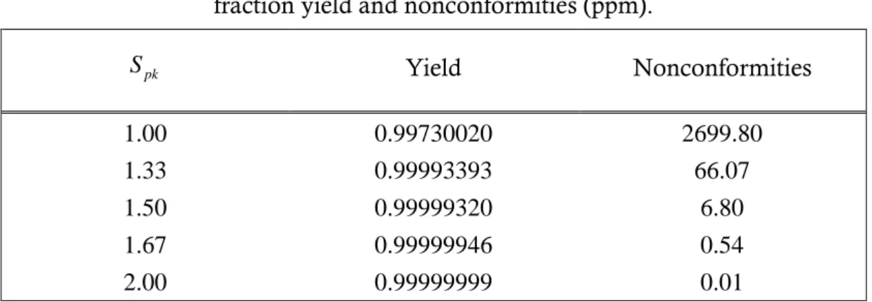
process yield. Table 1 summarizes the process yield, nonconformity (in ppm) as a function of the index Spk=1.00, 1.33, 1.50, 1.67, and 2.00. For example, if a particular process the yield measure Spk=1.67, then the corresponding value of nonconformities is 0.544 ppm.

Table 1. Some S_pk values and the corresponding values of

fraction yield and nonconformities (ppm). pk S _{Yield Nonconformities} 1.00 0.99730020 2699.80 1.33 0.99993393 66.07 1.50 0.99999320 6.80 1.67 0.99999946 0.54 2.00 0.99999999 0.01

2.3 Supplier Selection Problems based on PCIs

Because of the process mean  and the process variance  are not2

known in real world. In order to calculate the estimator, however, data must be collected to calculate the index value, and a great degree of uncertainty may be introduced into capability assessments due to sampling errors.

The most common methods to assess the process capability are to utilize the interval estimation and hypotheses testing. Consequently, these estimating methods must be performed by using their sampling distributions. Kotz and Johnson (2002) presented a thorough review for the PCI developments during the years 1992 to 2000. Spiring et al. (2003) consolidated the research findings of process capability analysis for the period 1990–2002. Lee et al. (2002) considered an asymptotic distribution for an estimate Spk



of the process yield index Spk. A useful approximate distribution of Spk



was furnished. Pearn and Chuang (2004) investigated the accuracy of the natural estimator of S_pk computationally, using

a simulation technique to find the relative bias and the relative mean square error for some commonly used quality requirements. Chen (2005) considered to use the bootstrap simulation technique to find four approximate lower confidence limits for index Spk. The simulation results show that the SB method significantly outperforms than other three methods. But, these studies considered the assessment of capability for a single process or supplier.

In a review of the problems for supplier selection based on PCIs, Tseng and Wu (1991) considered the problem for K available manufacturing processes based on the precision index Cp under a modified likelihood ratio (MLR) selection rule. Chou (1994) designed testing procedures for comparing two processes or suppliers in terms of Cp, Cpl, and Cpu when sample size are equal. Huang and Lee (1995) considered the supplier selection problem based on the index C_pm

and developed a mathematically approximation method for selecting a subset containing the process associated with the smallest s2 ₍m _T)2 from K given

the sample size required for a designated selection power. A two-phase selection procedure was developed to select a better supplier and to calculate the magnitude of the difference between two suppliers. Chen and Chen (2004) used four approximate confidence interval methods to present and compare for index Cpm. One based on the statistical theory given in Boyles (1991), and three based on the bootstrap (referred to as standard bootstrap, percentile bootstrap, and biased-corrected percentile bootstrap) for selecting a better supplier. However, the testing procedure for supplier selection based on Spk has not been done today. In this thesis, because the exact sampling distribution of Spk is analytical intractable, we will use bootstrap method to compare two processes based on

pk

3. Selection Method

3.1 Selecting a Better Supplier by Comparing Two Spk

One of the purposes of the process capability indices can be put to use is to select between competing processes that which is more capable. Since we do not have direct observation of the entire processes, we have no idea that which process is more capable. When we have samples of product provided by two suppliers, we may use the sample data to select the supplier whose product is better. We may switch to a new supplier if we can be sure that the process capability index of the new supplier is higher than that of the present supplier.

In this thesis, we investigate the selection problem with two candidate processes based on the index Spk. Let x11,x12,...,x1n and x21,x22,...,x2n be the measurements of two samples independently drawn from the normal distribution

2

1 1

( , )

N   and N(  , respectively. In general, if a new supplier #2 (S2)2, 22)

wants to compete for the orders by claiming that its capability is better than the existing supplier #1 (S1), the new S2 has to convince purchaser with a prescribed confidence level information to justify the claim. Thus, the supplier selection decision would be based on the hypothesis testing comparing the two Spk values.

It is

0: pk1 pk2

H S S

1: pk1 pk2

H S S _.

If the test rejects the null hypothesis H0:Spk1Spk2, then one has sufficient

information to conclude that the new S2 is better than the original S1, and the decision of the replacement would be suggested. This hypothesis testing problem can also be written as:

0: pk2 pk1 0

H S S  versus H1:Spk2Spk1 (difference testing)0 0: pk2/ pk1 1

H S S  versus H1:Spk2/Spk11 (ratio testing).

Therefore, if the lower confidence bound of Spk2Spk1 is positive in difference

testing, we can conclude that S2 has a better process capability than S1. Otherwise, we have no sufficient information to conclude that the S2 has a better process capability than S1. Similarly, if the lower confidence bound for the ratio between two process capability indices Spk2/Spk1 is larger than 1, then S2 has a better

process capability than S1. Otherwise, we have no sufficient information to conclude that the S2 has a better process capability than S1.

natural estimator Spk



, involving the statistics n_{1 i}/

i

x



_x n , and

2 1/ 2

1

[ n_i ( i ) /( 1)]

s



_ x x n are the sample mean and the sample standard

deviation being the conventional estimators of  and , respectively, obtained from a well-controlled process. The estimator is evidently

1 1 1 1 { ( ) ( )} 3 2 2 pk USL x x LSL S s s          .

Even under the normal distribution, the exact distribution of Spk



is mathematically intractable. Consequently, testing the process performance can not be accomplished. Lee et al. (2002) obtained an approximate distribution of

pk S



using the Taylor expansion technique. The estimator Spk

 can be expressed approximately as: 1 1 1 [ (3 )] ( ) 6 pk _{pk pk p} S S S W O n n        , where 3 1 1 1 1 (1 ) (1 ) 2 d Z W Y                         _ _{ }  _{ }_{   } _              ,

and above   ( m) /d ,   / d , (.) is the probability density function (p.d.f) of the standard normal variable N(0,1). O np( 1)

 _{represents the error of}

the expansion having a leading term of order 1

n in probability. It is noted that

the asymptotic expansion of Spk



is normally distributed with mean Spk and

variance 2 2 2 (a b ) / 36 ( (3n S_pk)) , where (1 ) 1 (1 ) 1 2 d a              _ _{ }  _{ }      , 1 1 b           _{  } _      .

Moreover, using rather complicated algebraic manipulations, Pearn et al. (2004) showed that, the estimator Spk



can be expressed in the form of:

2 2 1 2 3 4 5 1 ( )         pk _{pk p} S S D Z D Y D Z D ZY D Y O n n ,

here Z and Y are distributed according to the joint bivariate normal distribution,

and Di, i1, 2,..., 5, are functions of   ( m) /d and   / d. Therefore,

the distribution of S



polynomial combination of the distributions of Z and Y:



2



2 1 0 ( , ) (0, 0), , 0 1/ 2 d Z Y N where  _  





with the bias approximated as: 2 2

1 2 3 4 5

D ZD Y D Z D ZYD Y .

Both of these approximations to the distribution of Sˆpk are rather complicated and tedious. Undoubtedly, the distributions of Sˆpk2Sˆpk1 or

2 1

ˆ _/ ˆ

pk pk

S S and the constructions of exact confidence intervals for Sˆ_pk2Sˆ_pk1 and

2 1

ˆ _/ ˆ

pk pk

S S are much more difficult.

3.2 Bootstrap Methodology

Traditionally, statistical research work has relied on the central limit theorem and normal approximations to obtain standard errors and confidence intervals. These techniques are valid only when the statistic, or some known transformation of statistic, is asymptotically normal distribution. Unfortunately, most process data in real world are not normal distributed. More than that, the distribution of data is usually unknown. A major motivation for the traditional reliance on normal-theory methods has been computational tractability. Access to powerful computation enables the use of statistics in new and varied way. Idealized models and assumptions can now be replaced with more realistic modeling or by virtually model-free analyses. Efron (1979, 1982) introduced a nonparametric, computational intensive but effective estimation method, called the “Bootstrap”, which is a data based simulation technique for statistical inference. One can use the nonparametric bootstrap method to estimate the sampling distribution of a statistic, while assuming only that the observations are independent and identically distributed. The merit of the nonparametric bootstrap approach is that it does not rely on any assumptions regarding the underlying distribution. Rather than using distribution frequency tables to compute approximate p probability vales, the bootstrap method generates a unique sampling distribution based on the actual sample rather than the analytic method.

Most of PCIs literature concluded that the performance of bootstrap limits for PCIs are quite satisfactory in the majority of the cases. After Efron (1979, 1982) introduced the bootstrap, Efron and Tibshirani (1986) further developed three bootstrap confidence intervals: the standard bootstrap (SB) confidence interval, the percentile bootstrap (PB) confidence interval, and the biased-corrected percentile bootstrap (BCPB) confidence interval. Franklin and Wasserman (1991) proposed an initial study of these three methods for obtaining confidence intervals for Cpk when the process was normal distributed. Franklin and Wasserman (1992) also offered three bootstrap lower confidence limits for index Cp, Cpk, and Cpm. They compared the confidence interval from bootstrap

and from parametric estimates. The simulation results show that, the bootstrap confidence limits perform as good as the lower confidence limits derived by the parametric method in the normal process environment. (see Chou et al (1990) for

p

C , Bissell (1990) for Cpk, and Boyles (1991) for Cpm). These studies indicate that the bootstrap limits for PCIs are satisfactory in the cases.

In this thesis, the following four bootstrap confidence limits are employed to determine the lower confidence bounds of difference and ratio statistics and the results are used to select the better supplier of the two candidates. For n1=n2=n,

let two bootstrap samples of size n drawn with replacement from the two original

sample be denoted by



* * *



11 21, ,..., 1n x x x and



* * *



21 22, ,..., 2n x x x . The bootstrap sample statistics * 1

x , s₁*, x₂*, and s₂* are computed, as well as Sˆ*_pk1, and Sˆ*_pk2. A random sample of _nn _{possible resamples are drawn, the statistic is calculated}

by each of these, and the resulting empirical distribution is referred to as the bootstrap distribution of statistic. Due to the overwhelming computation time, it is not of practical interest to chose _nn _{such samples. Empirical work (Eforn and}

Tibshirani (1986)) indicated that a roughly minimum of 1,000 bootstrap resamples is usually sufficient to compute reasonable accurate confidence interval estimates for population parameters. For accuracy purpose, we consider B=3,000 bootstrap resamples (rather than 1,000). Thus, we take B=3,000 bootstrap estimates _qˆ* ₌ * * 2 1 ˆ ˆ (Spk Spk ) or * * 2 1 ˆ ˆ (Spk /Spk ) of θ = Spk2Spk1 or Spk2/Spk1 ,

respectively, then order them from the smallest to the largest * * *

( ) 2 1 ( ) ˆ ₍ˆ ˆ ₎ l Spk Spk l    or * * * ( ) 2 1 ( ) ˆ ₍ˆ _/ ˆ ₎ l Spk Spk l   where _{l 1,2, , B}.

Four types of bootstrap confidence intervals, including the standard bootstrap confidence interval (SB), the percentile bootstrap confidence interval (PB), the biased corrected percentile bootstrap confidence interval (BCPB), and the bootstrap-t (BT) methods introduced by Efron (1981), and Efron and Tibshirani (1986) are conducted in this paper. The generic notation ˆ and areˆ*

the estimator of θ and the associated ordered bootstrap estimate. Construction of a two-sided 100(1 2 )% confidence limit will be described. We note that a lower 100(1)% confidence limit can be obtained by using only a lower limit. The formulation details for the four types of confidence intervals are displayed as follows.

[A] Standard Bootstrap (SB) Method

Form the B bootstrap estimates _qˆ_{( )}*_{l , l 1,2, , B, the sample average and}

the sample standard deviation can be obtained as

* ˆ q * ( ) 1 1 B _ˆ l l B _ q 



, 1 2 * * * 2 ( ) 1 1 _{ˆ ˆ} [ ] 1 B l l S B q q q   _  _  _{ }  _  



 . ˆ

distribution of qˆ is approximately normal. Thus, the 100(1 2 )% a SB confidence interval for θ can be constructed as

a q

q ˆ* *

[ z S , q ˆ* z S ,a q*]

where qˆis the estimator of θ for the original sample, and z is the upper  quantile of the standard normal distribution.

[B] Percentile Bootstrap (PB) Method

From the ordered collection of * ( )

ˆ l

 , l 1,2, , B, the  percentage and

1-  percentage points are used to obtain the 100(1 2 )% PB confidence interval forθ, * ( ) ˆ [_B , * ((1 ) ) ˆ _] B   _ .

[C] Biased-Corrected Percentile Bootstrap (BCPB) Method

While the percentile confidence interval is intuitively appealing, it is possible that cause sampling errors, the bootstrap distribution may be biased. In other words, it is possible that bootstrap distributions using only a sample of the complete bootstrap distribution may be shifted higher or lower than would be expected. A three steps procedure is suggested to correct for the possible bias (Efron, 1982). First, using the ordered distribution of  , calculate theˆ*

probability *

0 [ˆ

p P q qˆ]0 . Second, we compute the inverse of the cumulative

distribution function of a standard normal based upon p₀ as z₀ 1( )p₀ ,

0 (2 )

L

p  z za pU (2z0 za). Finally, executing these steps to obtain the

100(1 2 )% BCPB confidence interval * ( ) ˆ [_{p BL} , * ( ) ˆ ]_{p BU}  . [D] Bootstrap-t (BT) method

By using bootstrap method to approximate the distribution of a statistic of the form (q qˆ )/S_qˆ, the bootstrap approximation in this case is obtained by

taking bootstrap samples from the original data values, calculating the corresponding estimates  and their estimated standard error, hence finding theˆ*

bootstrapped T -values T (qˆ* qˆ)/S_q* . The hope is that the generated

distribution will mimic the distribution of T. The 100(1 2 )% BT confidence interval for  may constitute as

* * * ˆ ˆ [ t S_{ }, * * * ˆ 1 ˆ _{t S ]}    ,

where _t*

a and t1*a are the upper  and 1 quantiles of the bootstrap

t-distribution respectively, i.e. by finding the values that satisfy the two equations

* ˆ [( P q ˆ)/_S* _t*_] q a q a    and _{P q[(}ˆ* * * 1 ˆ)/Sq t a] 1 q  a

    , for the generated

4. Performance Comparisons of Four Bootstrap Methods

4.1 Simulation Layout Setting

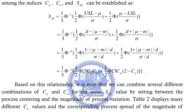
There are mainly two important characteristics, the process location relative to its specification limits, and the process spread in process capability. The closer the process location is to the mid-point of the specification limits and the smaller the process spread, the more capable the process is. A mathematical relationship among the indices Cp, Ca, and Spk can be established as:

1 1 1 1 { ( ) ( )} 3 2 2 pk USL LSL S             1 1 1 | | 1 | | { ( ) ( )} 3 2 2 d  m d  m             1 1 1 1 | | / 1 1 | | / { ( ) ( )} 3 2 / 2 / m d m d d d               1 1 1 1 { [3 ] [3 (2 )]} 3 2 C Cp a 2 Cp Ca        .

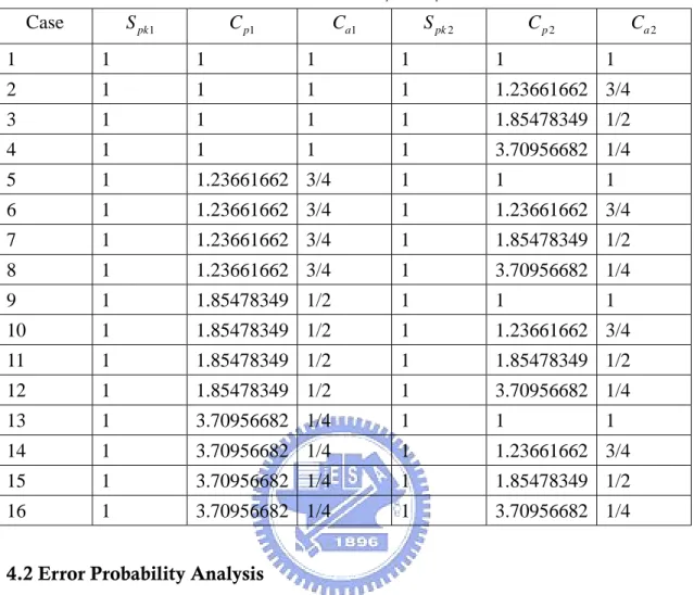
Based on this relationship, it is note that we can combine several different combinations of Cp and Ca for the same Spk value by setting between the process centering and the magnitude of process variation. Table 2 displays many different Ca values and the corresponding process spread of the magnitude of

.

Table 2. Ca values and ranges of .

a C value Range of m 1.00 a C  m m 0.75Ca 1.00 0 | m m |d/ 4 0.50Ca 0.75 d/ 4 | m m |d/2 0.25Ca 0.50 d/2 | m m | 3 / 4 d 0.00Ca 0.25 3 / 4 |d  m m |d 0.00 a C  m LSL orm USL 0.00 a C  m LSL orm USL

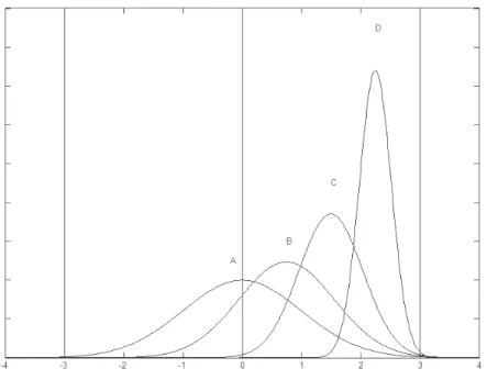
Figure 1. Four processes with Spk=1.00.

Figure 1 plots four process with difference combination of (C C_p, _a) withSpk 1.00, LSL=10, USL=20, and m=15. i.e. (C Cp, a)(1.00,1.00) for process

A, (C C_p, _a)(1.23661662, 0.75) for process B, (C C_p, _a)(1.85478349, 0.5) for

process C, (C Cp, a)(3.70956682, 0.25) for process D. These four processes have equivalent S_pk 1.00, and all have yields equal to 99.73%, but constructed with different  and . Hence, in order to make a comparative study among four bootstrap confidence limits, we take series of simulations to investigate the error probability and the selection power of difference and ratio testing statistics for the performance comparisons of four bootstrap methods. The setting values of parameters for two manufacturing suppliers used in the simulation study are given in Table 3. We investigate the performance of the methods with selected parameters for a wide range of index values and in on-target and off-target processes. For each combination, we generate 3,000 random samples, and the corresponding bootstrap confidence intervals for each of these samples are assessed in section 4.2.

Table 3. The parameter setting values for two manufacturing suppliers used in the simulation study under Spk1Spk2 1.00.

Case S_pk1 C_p1 C_a1 S_pk2 C_p2 C_a2 1 1 1 1 1 1 1 2 1 1 1 1 1.23661662 3/4 3 1 1 1 1 1.85478349 1/2 4 1 1 1 1 3.70956682 1/4 5 1 1.23661662 3/4 1 1 1 6 1 1.23661662 3/4 1 1.23661662 3/4 7 1 1.23661662 3/4 1 1.85478349 1/2 8 1 1.23661662 3/4 1 3.70956682 1/4 9 1 1.85478349 1/2 1 1 1 10 1 1.85478349 1/2 1 1.23661662 3/4 11 1 1.85478349 1/2 1 1.85478349 1/2 12 1 1.85478349 1/2 1 3.70956682 1/4 13 1 3.70956682 1/4 1 1 1 14 1 3.70956682 1/4 1 1.23661662 3/4 15 1 3.70956682 1/4 1 1.85478349 1/2 16 1 3.70956682 1/4 1 3.70956682 1/4

4.2 Error Probability Analysis

The error probability is the first step which we want to investigate. It is the proportion of times that reject the null hypothesis H0:Spk1Spk2 , while

0: pk1 pk2

H S S is true. Thus, we will calculate the proportion of times that the

lower confidence bound of Spk2Spk1 is positive and the lower confidence bound

of Spk2/Spk1 is larger than 1 for each case given in Table 2. We set sample size

n=100 drawn with replacement , the bootstrap resamples B=3,000, and the single simulation is replicated N=3,000 times. We usually set that the probability of the error selection less than a maximum value , referred to the  condition. The frequency of the error is a binomial random variable with N=3,000 and =0.05.

Thus, the 99% confidence interval for the error probability is

* * *

0.005 (1 )/

Z N

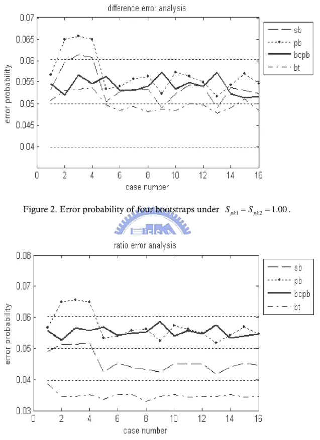
a   a a 0.05 2.576  (0.05 0.95)/ 3000 0.05 0.0103 . That is, one can have a 99% confidence that a “true 0.05 error probability”would have a range from 0.0397 to 0.061. Figure 2 and 3 show that the error probability of the four bootstrap methods for the difference and the ratio statistics with 16 different combination cases tabulated in Table 3.

Figure 2. Error probability of four bootstraps under Spk1 Spk2 1.00.

Figure 3. Error probability of four bootstraps under Spk2/Spk11.00.

difference statistic. There is only one occurrence out of the interval for SB method. We can note that with BCPB and BT methods, there is no case out of the control limit. That is, for different combinations of Cp and Ca for equal Spk value have no significant effect in error probability with BCPB and BT methods.

As for the ratio statistic in Figure 3, there are three cases out of the control limit (0.0397, 0.061) for the PB method. For the BT method, all of these cases are behind the lower control limit. That is, BT is a conservative bootstrap method for ratio statistic. With the SB and BCPB methods, there is no occurrence out of the interval. Table 4 and 5 show the results of error probability analysis for difference and ratio test. It means that, for different combinations of Cp and Ca for equal

pk

S value have no significant effect in error probability with SB and BCPB

methods.

Table 4. The results of error probability analysis for difference test. Bootstrap

method of difference test

Mean of these 16

cases error Standarddeviation of these 16 cases error

Number of out of limits

Out of limits case

SB 0.053895 0.003684 1 3

PB 0.056896 0.004436 3 2,3,4

BCPB 0.054166 0.001966 0 None

BT 0.049917 0.001934 0 None

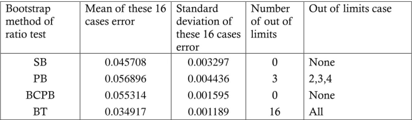
Table 5. The results of error probability analysis for ratio test. Bootstrap

method of ratio test

Mean of these 16

cases error Standarddeviation of these 16 cases error

Number of out of limits

Out of limits case

SB 0.045708 0.003297 0 None

PB 0.056896 0.004436 3 2,3,4

BCPB 0.055314 0.001595 0 None

BT 0.034917 0.001189 16 All

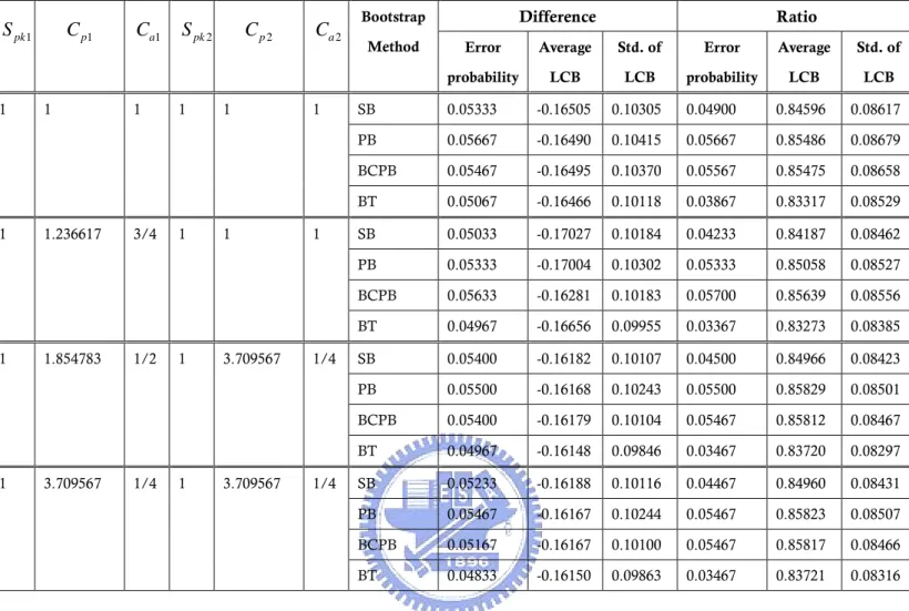
Besides that, an average lower confidence bound and the standard deviation of the lower confidence bound were calculated based on the N=3,000 different trials. Table 6 takes four of sixteen cases to show that the average lower confidence bound and the standard deviation of the lower confidence bound for each of the four different bootstrap methods. The results of all cases are summarized in Table 12.

Table 6. Simulation results of the four bootstrap methods for the difference and ratio statistics.

Difference Ratio 1 pk S C_p1 C_a1 S_pk2 C_p2 C_a2 Bootstrap Method Error probability Average LCB Std. of LCB Error probability Average LCB Std. of LCB 1 1 1 1 1 1 SB 0.05333 -0.16505 0.10305 0.04900 0.84596 0.08617 PB 0.05667 -0.16490 0.10415 0.05667 0.85486 0.08679 BCPB 0.05467 -0.16495 0.10370 0.05567 0.85475 0.08658 BT 0.05067 -0.16466 0.10118 0.03867 0.83317 0.08529 1 1.236617 3/4 1 1 1 SB 0.05033 -0.17027 0.10184 0.04233 0.84187 0.08462 PB 0.05333 -0.17004 0.10302 0.05333 0.85058 0.08527 BCPB 0.05633 -0.16281 0.10183 0.05700 0.85639 0.08556 BT 0.04967 -0.16656 0.09955 0.03367 0.83273 0.08385 1 1.854783 1/2 1 3.709567 1/4 SB 0.05400 -0.16182 0.10107 0.04500 0.84966 0.08423 PB 0.05500 -0.16168 0.10243 0.05500 0.85829 0.08501 BCPB 0.05400 -0.16179 0.10104 0.05467 0.85812 0.08467 BT 0.04967 -0.16148 0.09846 0.03467 0.83720 0.08297 1 3.709567 1/4 1 3.709567 1/4 SB 0.05233 -0.16188 0.10116 0.04467 0.84960 0.08431 PB 0.05467 -0.16167 0.10244 0.05467 0.85823 0.08507 BCPB 0.05167 -0.16167 0.10100 0.05467 0.85817 0.08466 BT 0.04833 -0.16150 0.09863 0.03467 0.83721 0.08316

4.3 Selection Power Analysis

After the error probability analysis, we can roughly ensure that, there is less effect for different combinations of C_p and C_a for equal S_pk value with

difference and ratio statistic. In order to compare the performance of these four bootstrap methods, we conduct further simulations of selection power with different sample sizes n=30(10)200 for Spk11.00, and Spk2 1.05(0.05)1.50. The

selection power calculates the probability of rejecting the null hypothesis

0: pk1 pk2

H S S while actually H1:Spk1Spk2 is true. For the difference statistic,

the selection power computes the proportion of times that the lower confidence bound of Spk2Spk1 is positive in the simulation. Similarly, for the ratio statistic,

the selection power computes the proportion of times that the lower confidence bound of Spk2/Spk1 is larger than 1. Figures 4-5 show the power of the four

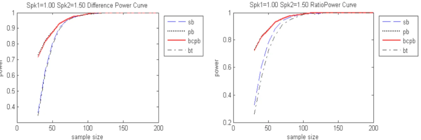
bootstrap methods for the difference and ratio statistic with sample size n=30(10)200 , Spk11.00 , Spk2 1.50 , respectively. The power curves for

1 1.00

pk

Figure 4. The selection power of the four bootstrap methods for the difference statistic with sample size n=30(10)200.

Figure 5. The selection power of the four bootstrap methods for the ratio statistic with sample size n= 30(10)200.

In Figure 4 and Figure 5, we find that PB and BCPB methods are much powerful under the same sample size. On the contrary, SB and BT methods have larger required sample size with fixed selection power. Under the two considerations of error probability above and selection power analysis, the BCPB method has more correct error probability and better selection power with fixed sample size. Consequently, we recommend the best of these four bootstrap methods is the BCPB method.

5. Supplier Selection Based on BCPB Method

5.1 Sample Size Determination with Designated Selection Power

In general, if a new supplier #2 (S2) wants to compete for the orders by claiming that its capability is better than the existing supplier #1 (S1), the new S2 has to convince purchaser with a prescribed confidence level information to justify the claim. Therefore, the sample size required for designated selection power must be determined to collect actual data from the factories. We investigate the BCPB method with B=3,000 bootstrap resamples, and the each simulation was then replicated with N=3,000 times. For convenience of applications, we tabulate the sample sizes required for various designated selection power = 0.90, 0.95, 0.975, and 0.99 under error probability 0.05. The selection power calculates the probability of rejecting the null hypothesis H0:Spk1Spk2 while actually

1: pk1 pk2

H S S is true. Tables 7-8 show the sample size required of the BCPB

method for the difference with Spk11.00 and Spk2 1.10(0.05)1.50 and ratio

statistics with Spk2 1.10(0.05)1.50. We also calculate the sample size required

for Spk11.30 and Spk2 1.40(0.05)1.80 for difference and ratio statistics in

Table 9 and 10.

Table 7. Sample size required of BCPB method for the difference statistics under 0.05  , with power = 0.90, 0.95, 0.975, 0.99, Spk11.00, Spk2 1.10(0.05)1.50.

S

pk1

S

pk2

1

1.1

1

1.15

1

1.2

1

1.25

1

1.3

1

1.35

1

1.4

1

1.45

1

1.5

90%

941 444 257 171 125 95 77 63 53

95%

1188 541 332 217 155 121 97 80 67

97.5%

1400 666 397 265 184 143 113 100 81

99%

1777 807 463 333 228 184 133 115 93

Table 8. Sample size required of BCPB method for the ratio statistics under 0.05  , with power = 0.90, 0.95, 0.975, 0.99, Spk11.00, Spk2 1.10(0.05)1.50.

S

pk1

S

pk2

1

1.1

1

1.15

1

1.2

1

1.25

1

1.3

1

1.35

1

1.4

1

1.45

1

1.5

90%

938 443 263 169 126 95 76 63 51

95%

1191 563 326 219 151 118 96 81 66

97.5%

1416 666 401 257 189 139 116 94 81

99%

1716 822 469 304 233 184 150 116 96

Table 9. Sample size required of BCPB method for the difference statistics under 0.05  , with power = 0.90, 0.95, 0.975, 0.99, Spk11.30, Spk2 1.40(0.05)1.80.

S

pk1

S

pk2

1.3

1.4

1.3

1.45

1.3

1.5

1.3

1.55

1.3

1.6

1.3

1.65

1.3

1.7

1.3

1.75

1.3

1.8

90%

1596 713 415 271 195 146 117 92 78

95%

1916 891 521 354 251 190 155 125 102

97.5%

2350 1088 643 413 338 230 176 147 119

99%

2925 1350 763 525 382 279 227 178 150

Table 10. Sample size required of BCPB method for the ratio statistics under 0.05  , with power = 0.90, 0.95, 0.975, 0.99, Spk11.30,Spk2 1.40(0.05)1.80.

S

pk1

S

pk2

1.3

1.4

1.3

1.45

1.3

1.5

1.3

1.55

1.3

1.6

1.3

1.65

1.3

1.7

1.3

1.75

1.3

1.8

90%

1596 721 421 275 198 148 121 96 77

95%

1965 917 514 350 250 189 152 126 102

97.5%

2397 1124 652 424 313 239 185 144 124

99%

2829 1297 749 512 376 278 226 189 152

For the convenience of observation, Figures 6-9 depict sample size curves based on the four sample size tables, respectively.

Difference Sample Size forSpk1=1.00 0 1000 2000 3000 4000 5000 6000 1.1 1.15 1.2 1.25 1.3 1.35 1.4 1.45 1.5 S_pk2 S am pl e S iz e _0.99 0.975 0.95 0.90

Figure 6. The sample size curve for the difference statistic under 0.05, with power = 0.90, 0.95, 0.975, 0.99, S_pk1 1.00, S_pk2 1.10(0.05)1.50.

Ratio Sample size forS_pk1=1.00

0 1000 2000 3000 4000 5000 6000 1.1 1.15 1.2 1.25 1.3 1.35 1.4 1.45 1.5 Spk2 S am pl e S iz e 0.99 0.975 0.95 0.9

Figure 7. The sample size curve for the ratio statistic under 0.05, with power = 0.90, 0.95, 0.975, 0.99, S_pk1 1.00, S_pk2 1.10(0.05)1.50.

Difference Sample Size forSpk1=1.3 0 2000 4000 6000 8000 10000 1.4 1.45 1.5 1.55 1.6 1.65 1.7 1.75 1.8 Spk2 S am pl e S iz e 0.99 0.975 0.95 0.9

Figure 8. The sample size curve for the difference statistic under 0.05, with power = 0.90, 0.95, 0.975, 0.99, S_pk1 1.3, S_pk2 1.40(0.05)1.80.

Ratio Sample Size forSpk1=1.3

0 2000 4000 6000 8000 10000 1.4 1.45 1.5 1.55 1.6 1.65 1.7 1.75 1.8 Spk2 S am pl e S iz e 0.99 0.975 0.95 0.9

Figure 9. The sample size curve for the ratio statistic under 0.05, with power = 0.90, 0.95, 0.975, 0.99, S_pk1 1.3, S_pk2 1.40(0.05)1.80.

From these figures, we can note that the larger the value of the difference

2 1

pk pk

S S

  or the ratio Spk2/Spk1 between two suppliers, the smaller the

sample size required for fixed selection power. For fixed  or  and Spk1, the

the sample size required is very similar either for the difference or the ratio statistics. This phenomenon can be explained easily, since the smaller of the difference and the larger designated selection power, the more collected sample is required to account for the smaller uncertainty in the estimation.

5.2 Selecting the Better Supplier

In this supplier selection problem, the practitioner should set the present minimum requirement of Spk values, and the minimal difference  or the minimal ratio  must be differentiated between suppliers with designated selection power. The practitioner alternatively might check Tables 7-10 for the sample size required under error probability 0.05, with designated selection power = 0.90, 0.95, 0.975, 0.99. After that, based on the BCPB method, if the LCB of Sˆpk2Sˆpk1 is positive or the LCB of Sˆpk2/Sˆpk1 is greater than 1, then we

can conclude that the supplier #2 is better than the supplier #1. Otherwise, we do not have sufficient information to reject the null hypothesis H :S0 pk1 Spk2. That is, we would believe that the existing supplier #1 is better than the new supplier #2.

6. Application Example：Color Filter Supplier Selection

Thin-film transistor liquid-crystal display (TFT-LCD) is one of the potential module of the high-tech products in the communication, information and consumer electronics industries. The TFT-LCD consumes less energy and weighs less compared to a cathode-ray tube (CRT). Besides that, it has emerged as the most widely used display solution, due to its high reliability, viewing quality and performance, compact size and environment-friendly features.

The basic structure of a TFT-LCD panel may be thought of as two glass substrates sandwiching a layer of liquid crystal. The front glass substrate is fitted with a color filter, while the back glass substrate has transistors fabricated on it. When voltage is applied to a transistor, the liquid crystal is bent, allowing light to pass through to form a pixel. A light source is located at the back of the panel and is called a backlight unit. The front glass substrate is fitted with a color filter, which gives each pixel its own color. Figure 10 shows the combination of the structure.

Figure 10. The combination of TFT-LCD structure.

The color filter is the most key component for a TFT-LCD. Many companies invest in producing a larger color filter to reduce the production cost. Competition in this market is very fierce. The thickness of the color filter is one of the most important quality characteristics. If the thickness of color filter is not in control, the TFT-LCD product may result in a certain degree of aberration.

The example is taken from a TFT-LCD manufacturing company, located in a science-based industrial park in Taiwan. The company would like to determine which of the two color filter suppliers has better process capability. For a particular model of the color filter investigated, the USL of a color filter

and the target value of a color filter thickness is set to 0.63mm.

6.1 Data Analysis and Supplier Selection

For the supplier selection problem, the practitioner should input the minimal requirement of Spk value first. Second, the minimal difference of Spk between these two suppliers with a designated selection power has to be set. Then we could decide the sample size based on Tables 7-10. In this case, the upper specification limit is 0.7mm, the lower specification limit is 0.56mm, and the target value is 0.63mm. The minimal requirement for the color filter product is 1.00, and the minimal difference between these two suppliers is 0.3, with selection power 0.95. By checking Tables 7-10, the sample size required for the difference statistics is 155, and for the ratio statistics is 151. We take 155 samples for S1 and S2, respectively. All sample data for two suppliers are showed in tables 15-16.

Figure 11. Histogram of data S1. Figure 12. Histogram of data S2. Figures 11-12 show the histogram of the 155 samples for S1 and S2. We use Kolmogorov–Smirnov test to check if these two suppliers’data are normal distributed. The statistic d for S1 is 0.038, and the statistic d for S2 is 0.065. Because both of these two p-values are greater than 0.05, we can not reject the null hypothesis. Thus, we conclude that the sample data for the two suppliers can be regarded as normal processes. We calculate the sample means, sample standard deviations, and the sample estimators ˆSpk for S1 and S2, summarized in Table 11.

Table 11. The calculated sample statistics for two suppliers.

x s Sˆ_pk

S1 0.630129 0.022558 1.0344

We execute the Matlab program to obtain the LCB for the difference between these two processes Sˆpk2Sˆpk1 is 0.09357, and the LCB for the ratio Sˆpk2/Sˆpk1 is

7. Conclusions

Supplier selection problem is an important issue in the manufacturing industry. The decision maker usually faces the problem of selecting the better supplier between two candidates. For most manufacturing factories, process yield is the fundamental criterion for supplier selection. The index Spk provides an exact measure on the process yield. However, the supplier selection problem based on index Spk has not been done.

In this thesis, we compared the performance of Spk2-Spk1 and Spk2/Spk1

with four different bootstrap methods including the standard bootstrap (SB), the percentile bootstrap (PB), the biased-corrected percentile bootstrap (BCPB), and the bootstrap-t (BT) methods. In error probability analysis, we found that SB and BCPB methods have stable error probabilities for both difference and ratio test. PB and BCPB methods are much powerful under the same sample size in selection power analysis. Thus, the performance of BCPB method is better than the other three methods. Forpractitioner’sconvenience,the useful information about the sample size required with designated selection power based on the BCPB method was tabulated. After that, we investigated a real world case on the color filter manufacturing process, and demonstrated the applicability of the proposed method step by step in the end.

References

1. Bissell, A. F. (1990). How reliable is your capability index? Applied Statistics, 39(3), 331-340.

2. Boyles, R. A. (1991). The Taguchi capability index. Journal of Quality Technology, 23, 17-26.

3. Boyles R. A. (1994). Process capability with asymmetric tolerances. Communication in statistics: Simulation and Computation, 23(3), 615-643.

4. Chan, L. K., Cheng S. W. and Spiring F. A. (1988). A new measure of process capability: Cpm. Journal of Quality Technology, 20, 162-173.

5. Chen, J. P. and Chen K. S. (2004). Comparing the capability of two processes using Cpm. Journal of Quality Technology, 36(3), 329-335.

6. Chen J. P. (2005). Comparing four lower confidence limits for process yield index Spk. The International Journal of Advanced Manufacturing Technology, 26, 609-614.

7. Choi, K. C., Nam K. H. and Park D. H. (1996). Estimation of capability index based on bootstrap method. Microelectronics Reliability, 36(9), 1141-1153.

8. Chou, Y. M., Owen, D. B. and Borrego, A. S. (1990). Lower confidence limits on process capability indices. Journal of Quality Technology, 22, 223-229.

9. Chou. Y. M. (1994). Selecting a better supplier by testing process capability indices. Quality Engineering, 6(3), 427-438.

10. Efron, B. (1979). Bootstrap methods: another look at the Jackknife. The Annals of Statistics, 7, 1-26.

11. Efron, B. (1982). The Jackknife, the bootstrap and other resampling plans. Philadelphia, PA.

12. Efron, B. and Tibshirani, R. J. (1986). Bootstrap methods for standard errors, confidence interval, and other measures of statistical accuracy. Statistical Science, 1, 54-77.

13. Efron, B. and Tibshirani, R. J. (1993). An Introduction to the Bootstrap. Chapman and Hall, New York.

14. Franklin L. A. and Wasserman G.S. (1991). Bootstrap confidence interval estimates of Cpk: An introduction. Communications in Statistics: Simulation and Computation, 20, 231-242.

15. Franklin, L. A. and Wasserman, G. S. (1992). Bootstrap lower confidence limits for capability indices. Journal of Quality Technology, 24(4), 196-210. 16. Hsiang, T. C. and Taguchi, G. (1985). A tutorial on quality control and assurance

-the Taguchi methods. ASA Annual Meeting, Las Vegas, Nevada.

17. Huang, D. Y. and Lee, R. F. (1995). Selecting the largest capability index from several quality control processes. Journal of Statistical Planning and Inference, 46, 335-346.

18. Juran, J.M. (1974). Quality Control Handbook (3rd Edition). McGraw-Hill, New York.

19. Kane,V. E. (1986). Process capability indices. Journal of Quality Technology, 18, 41-52.

20. Kotz, S. and Johnson, N. L. (2002). Process capability indices –a review, 1992-2000. Journal of Quality Technology, 34(1), 1-19.

21. Kushler, R. and Hurley, P. (1992). Confidence bounds for capability indices. Journal of Quality Technology, 24, 188-195.

22. Lee J. C., Hung H. N., Pearn W. L., Kueng T. L. (2002). On the distribution of the estimated process yield index Spk . Quality & Reliability Engineering International, 18(2), 111-116.

23. Pearn, W. L., Lin, G. H. and Chen, K. S. (1998). Distributional and inferential properties of process accuracy and process precision indices. Communications in Statistics: Theory & Method, 27(4), 985-1000.

24. Pearn, W. L. and Chuang, C. C. (2004). Accuracy analysis of the estimated process yield based on Spk . Quality & Reliability Engineering International, 20,305-316.

25. Pearn, W. L., Wu, C. W. and Lin, H. C. (2004). Procedure for supplier selection based on C_pm applied to super twisted nematic liquid crystal display processes. International Journal of Production Research, 42(13), 2719-2734.

26. Spiring, F., Leung, B., Cheng, S. and Yeung, A. (2003). A bibliography of process capability papers. Quality & Reliability Engineering International. 19(5), 445-460.

27. Tseng, S. T. and Wu, T. Y. (1991). Selecting the best manufacturing process. Journal of Quality Technology, 23, 53-62.

1 1 1 1 _S p k1 1 1 1 1 C p 1 1 1 1 1 _C a 1 1 1 1 1 _S p k2 3 .7 0 9 5 6 6 8 2 1 .8 5 4 7 8 3 4 9 1 .2 3 6 6 1 6 6 2 1 C p 2 1 /4 1/2 3/4 1 _aC 2 B T B C P B P B SB BT B C P B P B SB BT B C P B P B SB BT B C P B P B SB B o o ts tr ap U S L = 2 0 , L S L = 1 0 , d = 5 , m = 1 5 0 .0 5 3 6 7 0 .0 5 4 6 7 0 .0 6 5 0 0 0 .0 6 0 6 7 0 .0 5 3 3 3 0 .0 5 6 6 7 0 .0 6 5 6 7 0 .0 6 1 3 3 0 .0 5 3 0 0 0 .0 5 2 0 0 0 .0 6 5 0 0 0 .0 5 9 6 7 0 .0 5 0 6 7 0 .0 5 4 6 7 0 .0 5 6 6 7 0 .0 5 3 3 3 P -0 .1 5 9 5 1 -0 .1 6 3 8 1 -0 .1 5 6 4 9 -0 .1 5 6 5 9 -0 .1 5 9 5 6 -0 .1 6 3 8 5 -0 .1 5 6 5 6 -0 .1 5 6 6 5 -0 .1 5 9 6 7 -0 .1 6 3 8 7 -0 .1 5 6 8 1 -0 .1 5 6 8 6 -0 .1 6 4 6 6 -0 .1 6 4 9 5 -0 .1 6 4 9 0 -0 .1 6 5 0 5 L B o u n d 0 .1 0 0 6 8 0 .1 0 3 4 3 0 .1 0 4 1 6 0 .1 0 2 9 8 0 .1 0 0 6 5 0 .1 0 3 4 8 0 .1 0 4 2 6 0 .1 0 2 9 9 0 .1 0 0 7 6 0 .1 0 3 4 5 0 .1 0 4 2 9 0 .1 0 3 0 5 0 .1 0 1 1 8 0 .1 0 3 7 0 0 .1 0 4 1 5 0 .1 0 3 0 5 S td n = 1 0 0 (D if fe re n ce T es t) 0 .0 3 5 3 3 0 .0 5 5 6 7 0 .0 6 5 0 0 0 .0 5 1 6 7 0 .0 3 4 6 7 0 .0 5 6 6 7 0 .0 6 5 6 7 0 .0 5 1 3 3 0 .0 3 4 6 7 0 .0 5 2 6 7 0 .0 6 5 0 0 0 .0 5 1 3 3 0 .0 3 8 6 7 0 .0 5 5 6 7 0 .0 5 6 6 7 0 .0 4 9 0 0 P 0 .8 3 7 8 0 0 .8 5 6 6 3 0 .8 6 2 6 5 0 .8 5 3 8 4 0 .8 3 7 7 3 0 .8 5 6 5 3 0 .8 6 2 5 6 0 .8 5 3 7 8 0 .8 3 7 6 2 0 .8 5 6 4 9 0 .8 6 2 3 5 0 .8 5 3 5 9 0 .8 3 3 1 7 0 .8 5 4 7 5 0 .8 5 4 8 6 0 .8 4 5 9 6 L B o u n d 0 .0 8 5 0 5 0 .0 8 6 2 8 0 .0 8 7 1 5 0 .0 8 6 4 7 0 .0 8 4 9 8 0 .0 8 6 3 4 0 .0 8 7 1 9 0 .0 8 6 4 4 0 .0 8 5 0 9 0 .0 8 6 3 0 0 .0 8 7 2 5 0 .0 8 6 5 0 0 .0 8 5 9 2 0 .0 8 6 5 8 0 .0 8 6 7 9 0 .0 8 6 1 7 S td n = 1 0 0 (R at io T es t) T ab le 1 2 . T h e er ro r p ro b a b ili ty o f fo u r b o o ts tr ap m et h o d s fo r th e d if fe re n ce an d ra tio st at is tic w ith 1 6 co m b in at io n s o f ( C p 1_, C a 1₎ an d ( C p 2_, C a 2₎ u n d er S p k 1₌ S p k 2₌ 1 .0 0 .