Copula模式之下 雙變元存活資料之統計推論

國 立 交 通 大 學

統計學研究所

碩 士 論 文

Copula 模式之下 雙變元存活資料之統計推論

Statistical Inference for Bivariate

Survival Data Based on Copula Models

研 究 生：花文妤

指導教授：王維菁 教授

Statistical Inference for Bivariate Survival Data Based on

Copula Models

研 究 生：花文妤 Student：Hua, Wen-Yu

指導教授：王維菁 Advisor：Weijing Wang

國 立 交 通 大 學

統計學研究所

碩 士 論 文

A Thesis

Submitted to Institute of Statistics College of Science National Chiao Tung University

in Partial fulfillment of the Requirements for the Degree of

Master in Statistics June 2007

Hsinchu, Taiwan, Republic of China

Copula 模式之下 雙變元存活資料之統計推論

學生: 花文妤 指導教授: 王維菁 博士

國立交通大學統計研究所

摘要

本論文主要是考慮在 Copula 模式之下,雙變元存活資料受限於右設限之半 母數推論.目前存在許多估計相關性參數之半母數推論方法.我們比較三 種推論方法針對不存在解釋變數之同質性資料.並利用迴歸的概念將現有 的方法延伸至處理邊際異質的資料.最後,藉由模擬結果檢視上述方法之 有限樣本的表現. 關 鍵 字 : 雙 變 元 存 活 資 料 ;Cox 比 例 風 險 模 式 ; 相 關 存 活 時 間 ;Clayton 模 式;Copula 模式;半母數推論;二階段估計式;2×2 表格

Statistical Inference for Bivariate Survival Data

Based on Copula Models

Student: Hua, Wen-Yu Adivsor: Dr. Weijing Wang

Institute of Statistics Notional Chiao Tung University

Abstract

The thesis considers semi-parametric inference based on Copula models for bivariate survival data subject to right censoring. There exist several semi-parametric inference approaches to estimating the association parameter. We examine and compare three approaches developed for homogeneous data in absence of covariates. Then we extend these methods to a regression setting that accounts for marginal heterogeneity explained by the covariates. Finite-sample performances are examined by simulations.

Key words: Bivariate survival data; Cox proportional hazard model; Correlated

failure times; Clayton model; Copula model; Semi-parametric inference; Two-stage estimation; Two-by-two tables.

致謝

首先誠摯的感謝指導教授王維菁博士，老師悉心的教導使我得以一窺 統計領域的深奧，不時的討論並指點我正確的方向，使我在這兩年中獲益 匪淺。老師對學問的嚴謹更是我輩學習的典範。 兩年裡的日子，研究室裡共同的生活點滴，學術上的討論、言不及義 的閒扯、讓人又愛又怕的宵夜、趕作業的革命情感、因為睡太晚而遮遮掩 掩閃進教室...，要特別感謝我碩士班同學們，有你們的陪伴讓兩年 的研究生活變得絢麗多彩。 感謝 Takashi 學長、進見學長、秋婷學姐們不厭其煩的指出我研究中 的缺失，且總能在我迷惘時為我解惑，也感謝侑侑、怡君、小逼的幫忙， 讓我順利走過這兩年。益銘、建威、俊睿、永在以及吳志文，與你們一同 共進晚餐，是我準備碩士畢業及考試最開心的時光。 我男朋友、老莊在背後的默默支持更是我前進的動力，沒有老莊的體 諒、包容，相信這兩年的生活將是很不一樣的光景。 最後，謹以此文獻給我摯愛的家人，謝謝你們給我這個機會支持我體 諒我，讓我順利的完成碩士的學歷。 感謝這一路上曾經幫助過我的人，你們都是我生命中無法取代的貴人。 文妤 2007 年 6 月 交大統計所

Table of Content

Chapter 1 Introduction 1

1.1 Background 1

1.2 Notations and Outline of the Thesis 1

Chapter 2 Literature Review 3

2.1 Copula Models 3

2.2 Archimedean Copula Models 4

Chapter 3 Inference without Covariates 5

3.1 Estimation based on Martingale Residuals 5

3.1.1 Preliminary on Counting Processes and Martingales 5 3.1.2 Estimation of α 6

3.2 Two-Stage Estimation 8

3.3 Estimation based on Two-by-Two Tables 10

3.3.1 The Proposed Method 10

3.4 Discussion 12

Chapter 4 Inference with Covariates 13

4.1 Two-Stage Estimation 13

4.2 Estimation based on Two-by-Two Tables 15

Chapter 5 Simulations 16

5.1 Data Generation 16

5.1.1 Data Generation without Covariates 16

5.1.2 Date Generation with Covariates 17

5.2 Simulation Results 18

5.2.1 Results without Covariates 18

5.2.2 The Method Proposed by Hsu & Prentice 20

Chapter 6 Conclusion 23

References 30

Chapter 1 Introduction

1.1 Background

Multivariate survival analysis has wide applications in various fields. Consider an application in the study of familial aggregation for age onset data. The outcomes of age-at-onset within families may be correlated due to genetic and shared environmental risk factors among family members. Understanding the pattern of association may shed light on the disease etiology and is an important step useful for further scientific investigation.

Let (T ,...,₁ T_n) be the failure time variables for k members in a family. Note that T and _i

j

T for i≠ are often correlated. To simplify the analysis we let j k =2. In the thesis, we assume that (T1,T2) follows a copula model. The major goal is to estimate the association

parameter of the imposed model assumption based on right censored data. The situation for homogeneous data (i.e. without covariate information) will be discussed first. We will review existing methods and present our proposal. Then we will discuss a more complicated situation that includes the covariate information. Extension of the former inference methods will be discussed.

1.2 Notations and Outline of the Thesis

The failure times, T ,...,1 Tn, are subject to censoring by C ,...,1 Cn. Denoted the observed

data by {(X_1j,X_2j,δ_1j,δ_2j,Z_1j,Z_2j); j =1,2,..,n}, where, for an individual i , X is the _i

observed time and δ_i indicates the corresponding censoring status. If δ_i =1, X is _i

actually the observed failure time, T . Otherwise if i δi =0, X is the censoring time, i C . i

Let )Z_i :(p×1 be a vector of covariates for i=1,2. It is assumed that T and _i C are _i

independent.

In Chapter 2, we briefly review properties of copula models and introduce Archimedean copula models which constitutes a useful sub-family of copula models. Chapter 3 discusses

semi-parametric inference approaches to estimating the association parameter of a copula model in absence of covariates. Three methods will be examined in Section 3.1~3.3. In Section 3.4, we compare the three approaches.

In Chapter 4, we consider a more general situation in presence of covariates. Assuming that the covariates only affect the marginal distributions, we will extend the previous methods to account for marginal heterogeneity. In Chapter 5, we examine finite-sample performances of the methods via simulation studies. In Chapter 6, we give some concluding remarks. The appendix contains our further analysis about the estimator proposed by Hsu and Prentice (1996). Since this estimator does not have satisfactory performance in our simulations, we examine its computation algorithm in more detail to investigate the problem.

Chapter 2 Literature Review

2.1 Copula Models

Suppose that C is the joint survival function of two correlated U(0,1) random variables defined on the unit square [0,1]2. Let (T1,T2) be a pair of positive failure variables

with marginal survival functions (S1,S2)respectively. Note that if (T1,T2) are continuous,

both of S_i(T_i) for i=1,2 are distributed as U(0,1). Hence, the joint survival distribution function of (T1,T2) can be expressed as:

}. ) ( ), ( {S )) ( ), ( Pr( )) ( ) ( ), ( ) ( Pr( ) , Pr( ) , ( 2 2 1 1 2 2 2 1 1 1 2 2 2 2 1 1 1 1 2 2 1 1 2 1 t S t C t S U t S U t S T S t S T S t T t T t t S = ≥ ≥ = ≥ ≥ = ≥ ≥ = (2.1)

The above expression was names as a “copula model” by Sklar (1959). Notice that via the copula modeling, the space of joint analysis is transferred from [0,∞ to )2 [0,1]2. Hence copula models have been frequently used for describing the association between two failure variables which are often skewed. From the viewpoint of statistical inference, copula models have the nice feature that the dependence structure can be studied separately from the marginal distributions.

Usually the function C(u₁,u₂) is parameterized and denoted by C_α(u₁,u₂), where the parameter α measures the association between (T₁,T₂). Kendall’s τ is a rank-invariant association measurement, defined as

} 0 ) )( Pr{( } 0 ) )( Pr{( ₁*− _{1 2}*− ₂ ≥ − ₁*− _{1 2}*− ₂ < = T T T T T T T T τ , (2.2) where (T1,T2) and ( , ) * 2 * 1 T

T are independent but have the same distribution. The copula

parameter α is related to Kendall’s τ such that

1 ) , ( ) , ( 4 _{1 2} 2 1 2 1 2 2 1 _{∂ ∂} − ∂ =

_{∫ ∫}

dudu u u u u C u u C_α α τ . (2.3)

By equation (2.3), we see that there is a direct relationship between α and τ . For many well-known copula models, such a relationship has a nice one-to-one correspondence.

2.2 Archimedean Copula Models

The family of copula models has a useful sub-class, called the Archimedean copula (AC) family, in which Cα(u1,u2) can be further simplified as

)} ( ) ( { } , {u₁ u₂ 1 u₁ u₂ C_α =ϕ_α− ϕ_α +ϕ_α , (2.4) where )ϕ_α(u₁)+ϕ_α(u₂)≤ϕ_α(0 and ϕ_α(.):[0,1]→[0,∞] is the generating function

satisfying (1) 0 , ( ) ( ) 0 and ( ) ₂( ) 0 2 '' ' = < = > = dt t d t dt t d t α _α α α α ϕ ϕ ϕ ϕ

ϕ . The AC family has nice

analytic properties useful for more detailed investigation. Three examples of AC models are presented below:

(i) Clayton model (Clayton, 1978)

⎪⎩ ⎪ ⎨ ⎧ = > − + = − − − 1 if 1 if ) 1 ( ) , ( 2 1 1 1 1 2 1 1 2 1 α α α α α α u u u u u u C , and ) 1 /( ) 1 ( ) (ν ν1 α ϕ α α = − − − .

(ii) Frank model (Frank, 1979)

⎪ ⎩ ⎪ ⎨ ⎧ = < < ⎭ ⎬ ⎫ ⎩ ⎨ ⎧ ₊ − − = 1 if , 1 0 if , 1 -) 1 )( 1 ( 1 log ) , ( 2 1 2 1 2 1 α α α α α α α u u u u C u u , and )} 1 /( ) 1 log{( ) ( ν α ν α α ϕ = − − .

(iii) Positive stable frailty model (Hougaard, 1986)

⎪⎩ ⎪ ⎨ ⎧ = < < + = 1 if , 1 0 if , } }] )) (-log( ) g( exp{-[{-lo ) , ( 2 1 1 2 1 1 2 1 α α α α α α u u u u u u C , and α α ν ϕ 1 )} log( { ) ( = − v .

Chapter 3 Inference without Covariates

Consider a pair of failure times (T₁,T₂) which are assumed to be absolutely continuous.

In presence of right censoring, we only observe ( X1,X2,δ1,δ2 ), where

) 2 , 1 ( ) ( , = ≤ = ∧ =T C I T C i

X_{i i i} δ_{i i i} , and (C₁,C₂) are a pair of censoring times

independent of (T1,T2) . Observed data can be denoted as { (X1j,X2j,δ1j,δ2j) ,

( j=1,2,...,n)}. We assume that the joint survival function follows copula models: )]} ( [ )] ( [ { } ) ( ), ( { ) , Pr(T₁ ≥t₁ T₂ ≥t₂ =C S₁ t₁ S₂ t₂ =ϕ_α-1 ϕ_α S₁ t₁ +ϕ_α S₂ t₂ (3.1) The objective is to estimate α without specifying the marginal distributions.

In this chapter, we will review three semi-parametric inference approaches. In Section 3.1, we first review the concept of martingales which has been used by Hsu and Prentice (1996) to construct an estimating equation for estimating α . In Section 3.2, we review the paper of Shih and Louis (1995) who proposed a two-stage of estimation procedure. Specifically they suggest to estimate the marginal distribution first. Then these marginal estimates are treated as pseudo-observations of {S₁(T₁),S₂(T₂)} in the likelihood based on

(.,.)

α

C . In Section 3.3, we apply the idea of the Log-Rank statistic by constructing a series of two-by-two tables to estimate the association parameter. This idea has been used by Day et al. (1997) and Wang (2003) for analyzing semi-competing risks data.

3.1 Estimation based on Martingale Residuals

3.1.1 Preliminary on Counting Processes and Martingales

Based on observed variables, one can define N(t)= I(X ≤t,δ =1) which is a counting process and the filtrationFt =σ[N(u),I(T ≤u,δ =0);0≤u≤t], which describes the history of N(t) prior to or at time t .

Define the cumulative intensity process:

∫

≥ = Λ t tI X u u du 0 ( ) ( ) ) ( λ , (3.2) where

Δ ≥ Δ + ∈ = → Δ ) | ) , [ Pr( lim ) ( 0 u T u u T u λ

is the hazard of T at time u. Then define

) ( ) ( ) ( } { ) 1 , ( ) ( 0I X u u du N t t t X I t M = ≤ δ = −

∫

t ≥ λ = −Λ . (3.3)

According to the Doob-Meyer decomposition (Fleming and Harrington, 1991), the expectation of M(t) is a mean-zero martingale. Now we briefly verify the properties of

) (t

M :

(A) Given F which contains the history of the process prior the time of t , the expectation t

of dN(t) be an intensity process, such as:

) | 1 , Pr( ) ( ) | 1 , Pr( ) ( ) | ) ( (dN t F I X t X t T t I X t X t T t E t = ≥ = δ = ≥ + ≤ = δ = ≤ ). ( ) ( ) ( ) Pr( ) 1 , Pr( ) ( t d dt t t X I t X t X t X I Λ = ≥ = ≥ = = ≥ = λ δ (3.4)

(B) By the Doob-Meyer decomposition, the expectation of dM(t) equals to zero, such that: 0 ) | ) ( ) ( ( ) | ) ( (dM t Ft =E dN t −dΛ t Ft = E . (3.5) 3.1.2 Estimation of α

For the bivariate case, define

), ( ) ( ) ( ) ( ) 1 , ( ) ( 0I X u u du N t t t X I t M i i t i i i i i = ≤ δ = −

∫

≥ λ = −Λ (3.6)

where )λ_i(u is the hazard of T_i (i=1,2).When T₁ and T₂ are correlated, M₁(t₁) and

) ( 2 2 t

M are also correlated. Hsu and Prentice (1996) define the following cumulative

covariance function, or the covariance rate, as:

∫ ∫

= 1 2 0 0 1 2 2 1, ) ( , ) (τ τ τ τ ψ ψ dt dt , (3.7) where }. , | ) ( ) ( { ) , (dt₁ dt₂ = E M₁ dt₁ M₂ dt₂ T₁ ≥t₁ T₂ ≥t₂ ψ

The function ψ(τ1,τ2) contains the information of association and can be estimated either

A nonparametric estimator of ψ(dt1,dt2) is given by ) , ( ) ( ˆ ) ( ˆ ) , ( ˆ 2 1 ) , ( 2 2 1 1 2 1 2 1 t t r dt M dt M dt dt j R t t j j

∑

∈ = ψ , (3.8) where

∑

= ≥ ≥ = n j j j t X t X I t t r 1 2 2 1 1 2 1, ) ( , ) ( and Mˆ_i(t_i)= N_i(t_i)−Λˆ_i(t_i ∧T_i)(i =1,2). If (T₁,T₂) follow a copula model, the model-restricted version of ψ(t₁,t₂) can be expressed as:

∫ ∫

= 1 2 0 0 1 2 2 1, ; ) ( , ; ) (τ τ α τ τψ α ψ dt dt , (3.9) where )ψ(dt₁,dt₂;α)=ψ₀{S₁(t₁),S₂(t₂);α}Λ₁(dt₁)Λ₂(dt₂ and ) , ( ) , ( { } ; , { _{1 2} (11) _{1 2} (10) _{1 2} 0 u u α Cα u u Cα u u ψ = − 1 2 1 2 1 2 1 ) 01 ( ) , ( )} , ( ) , ( + − −C_α u u C_α u u C_α u u , ) , ( ) , ( 2 1 2 1 2 2 1 ) 11 ( u u u u C u u C ∂ ∂ ∂ = α α , 1 2 1 2 1 ) 10 ( ( , ) ) , ( u u u C u u C ∂ ∂ = α α and 2 2 1 2 1 ) 01 ( ( , ) ) , ( u u u C u u C ∂ ∂ = α α .

We have seen that, besides α , the model-based expression of the covariance function contains nuisance parameters. If the marginal functions S_i(t)andΛ_i(dt) (i=1,2) can be estimated, say by the Kaplan-Meier and Aalen’s estimators, respectively. One can estimate

) , (dt₁ dt₂ ψ by ) ( ˆ ) ( ˆ } ); ( ˆ ), ( ˆ { ) ; , (dt₁ dt₂ α =ψ₀ S₁ t₁ S₂ t₂ α Λ₁ dt₁ Λ₂ dt₂ ψ . (3.10)

Hsu and Prentice (1996) suggested the following estimating equation based on the weighted difference between the nonparametric estimator of ψ(t₁,t₂) and its model-based estimator:

0 )} ; , ( ˆ ) , ( ˆ { ) , ( ) ( ˆ 1 2 0 0 1 2 1 2 1 2 1 − = = −

_{∫ ∫}

τ τ _{ψ ψ α} α n r t t dt dt dt dt U_n . (3.11)

Example: the Clayton model

1 1 1 2 1 1 2 1, ) ( 1) ( = −α+ + −α+ − −α− α u u u u C (3.12)

∫ ∫

= 1 2 0 0 1 2 2 1, ; ) ( , ; ) (t t α t tψ du du α ψ , (3.13) where )ψ(du1,du2;α)=ψ0{S1(u1),S2(u2);α}Λ1(du1)Λ2(du2 and 2 1 1 1 1 2 1 2 1 1 1 2 1 1 2 1 0{ , ; } ( 1) ( 1) − + − + − − + − + − + − + − _{+ − − + −} =α α α α α α α α ψ u u u u u u u u . 3.2 Two-Stage Estimation

We can view Cα(u1,u2) as the joint survival function of (U1,U2)= (S1(T1),S2(T2)).

If one can obtain a random sample of (T₁,T₂), denoted as {(T_1j,T_2j),(j=1,2,..,n)}, and ) 2 , 1 ( ) (⋅ i =

S_i are completely specified, the likelihood of α can be written as

∏

= n j j j u u C 1 2 1 ) 11 ( ) , ( α , (3.14)

where ).uij =Si(tij)(i=1,2 j=1,2,...,n When (T1,T2) are subject to right censoring, the

likelihood of α can be modified as:

. ) , ( ) , ( ) , ( 1 2 (1 )(1 ) ) 1 ( 2 1 01 1 ) 1 ( 2 1 10 1j 2j 1j 2j 1j 2j j j j j n j j j u C u u C u u u C_α δ δ _α −δ δ _α −δ −δ = − × ×

∏

(3.15)

However, (S₁(T₁),S₂(T₂)) cannot be observed directly in practice. Shih and Louis (1995) propose a straightforward method to estimate α . The ideas are to estimate (S1(T1),S2(T2))

first and then plug in the likelihood function of α . There are two methods for estimating the marginal distribution. One is the parametric approach in which the marginal distributions are specified up to some unknown parameters. By applying the maximum likelihood approach for

estimating the marginal parameters, one can estimate (S1(X1),S2(X2)) by

)) ( ~ ), ( ~

(S₁ X₁ S₂ X₂ . The other approach does not assume the form of the marginal distributions, the Kaplan-Meier method can be applied for estimating S_i(T_i)(i =1,2). We illustrate this approach using the Clayton model as an example.

Example: the Clayton model

1 1 1 2 1 1 2 1, ) ( 1) ( = −α+ + −α+ − −α− α u u u u C (3.16)

∏

= − n j j j j j j j j j u u C u u C 1 ) 1 ( 2 1 ) 10 ( 2 1 ) 11 ( 1 2 1 2 ) , ( ) , ( δ δ _α δ δ α ) 1 )( 1 ( 2 1 ) 1 ( 2 1 ) 01 ( 1 2 1 2 ) , ( ) , ( j j j j j j j j u C u u u C_α δ −δ _α −δ −δ × , (3.17) where 2 1 1 1 2 1 1 2 1 2 1 ) 11 ( ) 1 ( ) , ( = × −α −α × −α+ + −α+ − −α− α u u α u u u u C , 1 1 1 1 2 1 1 1 2 1 ) 10 ( ) 1 ( ) , ( = −α × −α+ + −α+ − −α− α u u u u u C and 1 1 1 1 2 1 1 2 2 1 ) 01 ( ) 1 ( ) , ( = −α× −α+ + −α+ − −α− α u u u u u C .

In presence of censoring, we observe{(X1j,X2j,δ1j,δ2j) (j=1,2,...,n)}. If the marginal

distributions are specified, say exp(λ =1), the maximum likelihood estimator of Si(Xij) is

) ( ~ ij i X S , where n j i X X X S n ij j ij n j ij ij

i( ) exp( );for 1,2and 1,2,...,

~ 1 1 _{= =} − =

∑

∑

= = δ . (3.18)

If the marginal form is unknown, we estimate Si(Xi) by Kaplan-Meier estimator:

. ,..., 2 , 1 and 2 , 1 for ; ) ( ) 1 , ( 1 ) ( ˆ 1 1 n j i u X I u X I X S _n j ij n j ij ij x u ij i ij = = ⎪ ⎪ ⎭ ⎪⎪ ⎬ ⎫ ⎪ ⎪ ⎩ ⎪⎪ ⎨ ⎧ ≥ = = − =

∑

∑

Π

= = ≤ δ (3.19)

3.3 Estimation based on Two-by-Two Tables

3.3.1 The Proposed Method

In this section, we propose an estimator of α for an Archimedean Copula Models of the form:

)]}Pr(T₁ ≥t₁,T₂ ≥t₂)=C{S₁(t₁),S₂(t₂)}=ϕ_α-1{ϕ_α[S₁(t₁)]+ϕ_α[S₂(t₂ . (3.20) This idea is actually an application of the papers of Day et al. (1997) and Wang (2003) who considered semi-competing risks data. In presence of censoring, we observe

)}. ,..., 1 ( ) , , ,

{(X1j X2j δ1j δ2j j= n The proposed estimating procedure is related to the

Log-Rank statistic which can be constructed based on a series of two-by-two tables. At an observed failure points (t₁,t₂), we can construct the following two-by-two tables as follows:

Table: Two-by-Two Tables at time (t₁,t₂)

The cell counts are defined as follows. Let

∑

= = = = = = n j j j j j t X t X I dt dt N 1 2 2 2 1 1 1 2 1 11( , ) ( ,δ 1, ,δ 1),

∑

= ≥ = = = n j j j j t X t X I t dt N 1 2 2 1 1 1 2 1 10( , ) ( ,δ 1, ),

∑

= = = ≥ = n j j j j t X t X I dt t N 1 2 2 2 1 1 2 1 01( , ) ( , ,δ 1) and

∑

= ≥ ≥ = n j j j t X t X I t t R 1 2 2 1 1 2 1, ) ( , ) ( . 1 , 2 2 2 =t δ = X X2 >t2 1 , ₁ 1 1 =t δ = X N₁₁(dt₁,dt₂) N₁₀(dt₁,t₂) 1 1 t X > ) , (1 2 01 t dt N R(t1,t2)

Notice that the odds ratio of the table converges to ) , Pr( ) , Pr( ) , Pr( ) , Pr( ) , ( 2 2 1 1 2 2 2 1 1 1 2 2 1 1 2 2 1 1 2 1 2 2 1 t T t T t t T t T t t T t T t T t T t t t t ≥ ≥ ∂ ∂ ≥ ≥ ∂ ∂ ≥ ≥ ≥ ≥ ∂ ∂ ∂ = θ . (3.21)

For models in the AC family, θ(t₁,t₂) can be simplified as

)) , (Pr( ~ ) , (t₁ t₂ =θ_α T₁ ≥t₁ T₂ ≥t₂ θ , (3.22)

where θ~ ⋅_α() is an univariate function satisfying

) ( ) ( ) ( ~ v v v v α α α _ϕ ϕ θ ′ ′′ × − = . (3.23)

Conditioning on the marginal counts, N11(dt1,dt2)follows a hypergeometric distribution with

mean: ) , ( ) , ( ) , ( ) , ( ) , ( ) , ( ) , ( ) , , ( 2 1 10 2 1 2 1 10 2 1 2 1 01 2 1 10 2 1 2 1 11 t dt N t t R t dt N t t dt t N t dt N t t dt dt E − + = θ θ α (3.24) ) , ( ) , ( ) , ( ) , (Pr( ~ (Pr( , )) ( , ) ( , ) ~ 2 1 10 2 1 2 1 10 2 2 1 1 2 1 01 2 1 10 2 2 1 1 t dt N t t R t dt N t X t X dt t N t dt N t X t X − + ≥ ≥ ≥ ≥ = α α θ θ .

By equating the empirical count with its model-based expected value and combining the tables with different (t₁,t₂), we can construct the following estimating equation:

∫ ∫

− = = − 1 2 0 0 1 2 11 1 2 1 2 1 0 )} , , ( ) , ( ){ , ( ) (α n τ τ W t t N dt dt E dt dt α L , (3.25)

where W(t1,t2) is the weight function. It has been suggested to use

)) , ( ( )) , ( ( ) , ( 2 1 2 1 2 1 t t S t t S t t W α α θ θ& = , (3.26) where S(t1,t2)=Pr(T1 ≥t1,T2 ≥t2) and _α ν θ ν θ α α _∂ ∂ = ( ) ) ( & .

Example: the Clayton model

1 1 1 2 1 1 2 1, ) ( 1) ( = −α+ + −α+ − −α− α u u u u C (3.27)

For Clayton model with ϕ_α(t)=t−(α−1) −1,(α >1), we can obtain the model based expectation of N11(dt1, dt2):

) , ( ) , ( ) , ( ) , ( ) , ( ) , , ( 2 1 10 2 1 2 1 10 2 1 01 2 1 10 2 1 11 t dt N t t R t dt N dt t N t dt N dt dt E − + × × = α α α . (3.28) 3.4 Discussion

Shih and Louis (1995) proposed a two-stage estimation procedure. This approach is semi-parametric in the sense that the first stage can be estimated non-parametrically. However in some complicated data structures, such as semi-competing risk, nonparametric estimation in the first stage is not applicable. Hsu and Prentice (1996) constructed their estimating function based on martingale residuals. However the model-based expression involves too many high-dimensional nuisance parameters and therefore the resulting estimating equation becomes very complicated. Practical performance of this estimator heavily depends on the accuracy of the plug-in estimates in all data range. In our simulations, we have found that estimation in the tail region is not satisfactory.

The latter two approaches only use the conditions of the moments. It seems that the approach based on two-by-two tables is a more natural way for describing the dependence structure for AC models. Specifically for the Clayton model E11(dt1,dt2,α) does not even

contain any nuisance parameters. The key is that the theoretical odds ratio of the tables can well capture the association information for AC models. In contrast, ψ(t1,t2;α) is much less

natural. It involves high-dimensional nuisance parameters that affect the subsequent inference procedure.

Chapter 4 Inference with Covariates

In this chapter, we discuss the estimation of α when there exist covariates that may affect the marginal distributions. Let (T1,T2) and (C1,C2) be failure times and censoring

times, respectively. Let Z_i : p× i1( =1,2) be the covariate vectors. In presence of right censoring, observed data can be expressed as {(X1j,X2j,δ1j,δ2j, )}Z1j,Z2j),(j=1,2,...,n ,

whereXij =Tij∧Cij and δij =I (Tij <Cij), for i=1,2 and j = 1,2,...,n .

Here we assume that Z only affects i T i (i =1,2), marginally. Let

). 2 , 1 ( ) | Pr( ) | ( = ≥ = =S t Z T t Z i U_{i i i i i} (4.1)

Furthermore, we assume that

). , ( ) , Pr(U₁ ≥u₁ U₂ ≥u₂ =C_α u₁ u₂ (4.2) In the following analysis, we assume that marginally the covariate effect follow the Cox Proportional Hazard model, such that

), 2 , 1 ( ) exp( ) ( ) (t = i,0 t Zi' i i= i λ β λ (4.3)

where )λi,0(t is the baseline hazard function. In Section 4.1, we modify the two-stage estimation approach. In Section 4.2, we apply our idea based on two-by-two tables to handle this more generalized situation.

4.1 Two-Stage Estimation

The first stage involves estimating pseudo-observations of (U₁,U₂). Note that, under the Cox PH model,.U =S (t |Z )=S_,0(t )exp(Zi' i) (i=1,2).

i i i i i i β

This implies that we need to estimate βi and Si,0(ti) first. The regression parameter βi can be estimated by

maximizing the following likelihood

). 2 , 1 ( ) exp( ) ( ) exp( ) 1 , ( ) ( 1 1 ₌ ′ × ≥ ′ × = = =

∏

∑

∑

= = i Z u X I Z u X I L u failure i ij n j ij i ij n j j ij i β β δ β (4.4)

The estimator of the baseline function can be expressed by Breslow’s estimator: ). 2 , 1 ( ) ) ˆ exp( ) 1 , ( 1 ( ) ( ˆ ) ( ) ( } ' ) ( ) ( 0 , = = = − =

∑

∑

Π

∈ ≤ i Z t X I t S R t i j i t i j i t t i i j j i ii β δ (4.5)

Then we can obtain ₁ ˆ_1,0( ₁)exp(Z'βˆ1) and

T S U = U₂ = _{2,0 2} exp( ˆ2) ' ) ( ˆ _T Ziβ S . Based on ) , , ,

{(U_1j U_2j δ_1j δ_2j )}(j=1,2,...,n , we can estimate α by the following likelihood function: ) 1 ( 2 1 ) 10 ( 2 1 ) 11 ( 1 2 1 2 ) , ( ) , ( ) ( j j j j j j j j j j u u C u u C L α

Π

_α δ δ _α δ −δ

Π

= ). ,.., 1 ( ) , ( ) , ( _{1 2} (1 )(1 ) _{1 2} (1 )(1 ) ) 01 ( 1 2 1 2 n j u u C u u C j j j j j j j j = × _α −δ −δ _α −δ −δ (4.6)

For Clayton’s model with 1

1 1 2 1 1 2 1, ) ( 1) ( = −α+ + −α+ − −α− α u u u u

C , the above likelihood equals

) 1 ( 2 1 ) 10 ( 2 1 ) 11 ( 1 2 1 2 ) , ( ) , ( ) ( j j j j j j j j j j u u C u u C L α

Π

_α δ δ _α δ −δ

Π

= ). ,.., 1 ( ) , ( ) , ( _{1 2} (1 )(1 ) _{1 2} (1 )(1 ) ) 01 ( 1 2 1 2 n j u u C u u C j j j j j j j j = × _α −δ −δ _α −δ −δ (4.7) where 1 2 1 1 2 1 1 2 1 2 1 ) 11 ( ) 1 ( ) , ( = × −α −α × −α+ + −α+ − −α− α u u α u u u u C , 1 1 1 1 2 1 1 1 2 1 ) 10 ( ) 1 ( ) , ( = −α × −α+ + −α+ − −α− α u u u u u C and 1 1 1 1 2 1 1 2 2 1 ) 01 ( ) 1 ( ) , ( = −α× −α+ + −α+ − −α− α u u u u u C .

4.2 Estimation based on Two-by-Two Tables

Based on pseudo-observations {(U_1j,U_2j,δ_1j,δ_2j)(j=1,...,n)}, we can construct the following two-by-two table:

Table: Two-by-Two Table based on pseudo-observations

The cell counts are defined as follows. Let

∑

= = = = = = n j j j j j u U u U I du du N 1 2 2 2 1 1 1 2 1 11( , ) ( ,δ 1, ,δ 1),

∑

= ≥ = = = n j j j j u U u U I u du N 1 2 2 1 1 1 2 1 10( , ) ( ,δ 1, ),

∑

= = = ≥ = n j j j j u U u U I du u N 1 2 2 2 1 1 2 1 01( , ) ( , ,δ 1) and

∑

= ≥ ≥ = n j j j u U u U I u u R 1 2 2 1 1 2 1, ) ( , ) ( .

Accordingly the estimating function becomes:

∫ ∫

− = = − 1 2 0 0 1 2 11 1 2 1 2 1 0 )} , , ( ) , ( ){ , ( ) (α n τ τ W u u N du du E du du α L , (4.8) where ) , ( ) , ( ) , ( ) , ( ) , ( ) , ( ) , ( ) , , ( 2 1 10 2 1 2 1 10 2 1 2 1 01 2 1 10 2 1 2 1 11 u du N u u R u du N u u du u N u du N u u du du E − + = θ θ α .

Consider the Clayton model:

1 1 1 2 1 1 2 1, ) ( 1) ( = −α+ + −α+ − −α− α u u u u C . (4.9)

The above likelihood function of α can be simplified using the fact that θ(u₁,u₂)=α .

1 , ₂ 2 2 =u δ = U U₂ >u₂ 1 , ₁ 1 1 =u δ = U N₁₁(du₁,du₂) N₁₀(du₁,u₂) 1 1 u U > ) , ( _{1 2} 01 u du N R(u1,u2)

Chapter 5

Simulations

5.1 Data Generation

Via simulations, we will examine finite-sample performances of several estimators of α without and with covariates. We consider generating (T1,T2) from the Clayton model of the

form: ⎪⎩ ⎪ ⎨ ⎧ = > − + = − + − + − − ). 1 ( ) 1 ( ) 1 ( ) , ( 2 1 1 1 1 2 1 1 2 1 α α α α α α u u u u u u C (5.1)

Note that α =(1−τ)/2τ , where τ is Kendall’s τ . In particular, we will adopt the data generation algorithm for the Clayton model proposed by Prentice and Cai (1992).

5.1.1 Data Generation without Covariates

Step (i) Specify the value of τ and compute

τ τ α − + = 1 1 .

Step (ii) Generate independent variables {(U_1j,U_2j)(j =1,...,n)}, where U_ij ~ ) 2 , 1 ( ) 1 , 0 ( i= U .

Step (iii) Generate {(T1j,T2j)(j=1,2,...,n)}, such that:

, ) 1 ( 1 2 α γj = −U j − ], ) 1 ( 1 log[ 1 1 1 1 α γ γ α + − − + − × = j j j j U T . ) 1 ( 1 2 2 α − − = j j U T

Then (T1j,T2j) follows Clayton(α) and marginally Tij(i=1,2)~exp(1).

Step (iv) Generate {(C1j,C2j)(j=1,2,...,n)}, both of which are uniformly distributed.

Finally with {(T1j,T2j,C1j,C2j)(j=1,...,n)}, we can create observed data {(X1j,X2j,

)} ,..., 2 , 1 ( ) , ₂ 1j δ j j= n

5.1.2 Date Generation with Covariates

Now we generate data which include a binary covariate. We assume the marginal effect follows the Cox proportional hazard model (1972), such as:

, ) ( ) ( ,0 exp( ) ' i i Z i i t S t S = β (5.2) where Z is the covariate and _i S_i,0(t) is the baseline survival function at time t (i=1,2). The general procedure can be stated as follows. Let S(T)=U, where U ~ U(0,1), and under the Cox proportional hazard model, we have S₀(T)exp(Z′ )β =U. Hence it follows that

) exp( ) log( )) ( log( 0 _β Z U T S ′ = , (5.3) which implies that

⎥ ⎦ ⎤ ⎢ ⎣ ⎡ ′ = − ) ) exp( ) log( exp( 1 0 β Z U S T . (5.4)

We still need to specify the form of S₀(t). For most distributions, the inverse of S₀(t) may not have an explicit expression which increases the numerical difficulty in the analysis. In our simulations, we specify the baseline survival function to be S₀(t)=exp(−t) and obtain the following explicit expression:

) exp( ) log( β Z U T ′ − = , (5.5) where −log(U) which follows exp(1).

The data generation procedure is summarized below. Step (i) Generate Z from Bernoulli(0.5) for _ij i=1,2.

Step (ii) Generate failure times (T₁*_j,T₂*_j) for the baseline group with

0 =

ij

Z using the above algorithm, whereT_ij* ~exp(1)(i=1,2).

) exp( ' * i ij ij ij Z T T β = (i =1,2).

Step (iv) Generate {(C1j,C2j)(j=1,2,...,n)}, both of which are exponential distributed.

Finally with {(T1j,T2j,C1j,C2j,Z1j,Z2j)(j=1,...,n)} , we can create observed data

)} ,..., 2 , 1 ( ) , , , , ,

{(X_1j X_2j δ_1j δ_2j Z_1j Z_2j j= n such that X_ij =T_ij ∧C_ij and δ_ij = I(T_ij ≤C_ij).

5.2 Simulation Results

5.2.1 Results without Covariates

In this section, we evaluate two approaches based on two-stage estimation and the

construction of two-by-two tables. Two sample sizes with n=100 and n=500 are

considered. The parameter α ranges form 21. to 19 which correspond to τ from 0.1 to 0.9. For each estimator, the average bias and standard deviation of α are reported based on 500 replications. To achieve the targeted censoring rates, 30 % and 60 %, we set C to i

follow U(0,5.5) and U(0,2.5), respectively for i=1,2.

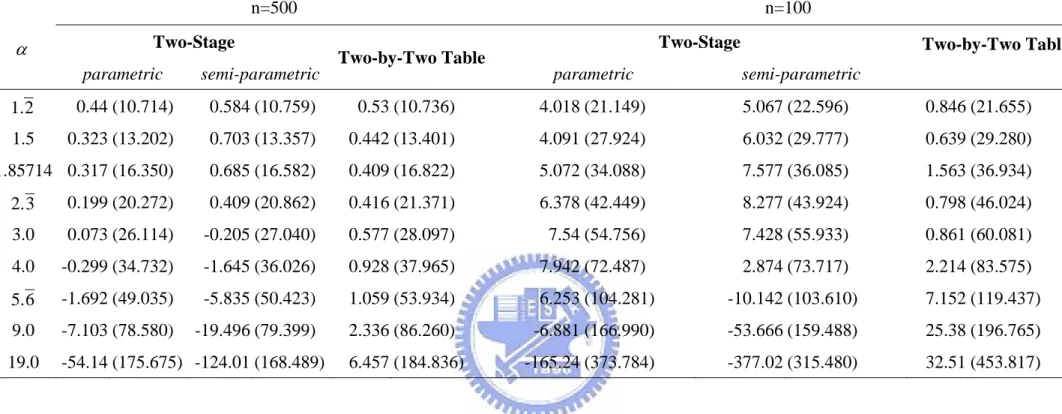
Table 1.1 summarizes the results in absence of censoring. Note that for the approach of two-stage estimation, we also present the results when the first stage of estimation is performed parametrically. Recall that we assume the marginal distribution of failure time X is exp(λ =1). Hence, for the parametric two-stage procedure, we use

∑

∑

= = = _n j j n j j x 1 1 ˆ δ

λ (in complete data

x

1 ˆ₌

λ ) (5.6)

to plug in the second stage for estimating α . This approach yields better results (smaller bias and smaller variation) than the semi-parametric two-stage procedure. As for the approach constructed based on two-by-two tables, it produces fairly nice results despite that it makes no assumption on the marginal distributions. Specifically it is fairly unbiased and the variance is only slightly larger than the parametric two-stage procedure. Note that the variation of all the

estimators becomes larger when α increases.

Table 1.2 and 1.3 are the results in presence of external censoring. Although variation of the estimators are larger than those without external censoring, the estimators still perform well. For Table 1.1 ~ 1.3, the variation is close to zero with the increasing of sample size (from 100 to 500). Hence, we can conclude that all of the estimations satisfy the property of consistency.

5.2.2 The Method Proposed by Hsu & Prentice

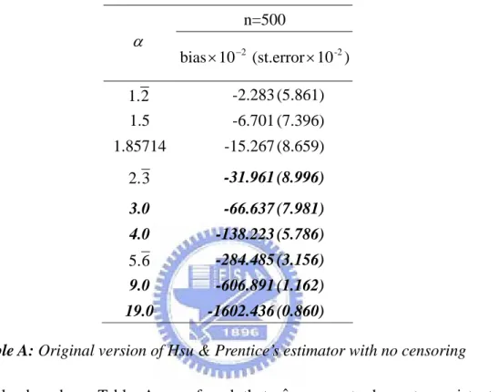
In this section, we examine the performance of the estimator proposed by Hsu and Prentice (1996) under the same settings. The results based on complete data are summarized below.

Strangely, based on Table A, we found that αˆ seems to be not consistent when

3 . 2 ≥

α . To investigate what caused the problem, we checked several things. The details are

summarized in the Appendix. We suspected that the problem may be attributed to the estimation instability of ψ(t1,t2;α) in (3.10) in some region of (t1,t2). The plugged-in

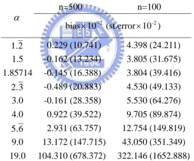
marginal estimators are usually unstable in the tail area. Hence we trimmed the integration area from [0,∞)×[0,∞) to a bounded region. Because this modification has no theoretical justification, we only evaluate the case without censoring.

Table B below contains the results for the modified estimator which is analyzed in a bounded region. Specifically, for each margin, we trim 50 % of the tail region. Based on Table B, we can know that both of bias and standard deviation of αˆ have significant improvement. With the sample size increases from 100 to 500, the standard deviation of αˆ have less

n=500 α ) 10 (st.error 10 bias× −2 × -2 2 1. -2.283 (5.861) 1.5 -6.701 (7.396) 1.85714 -15.267 (8.659) 3 2. -31.961 (8.996) 3.0 -66.637 (7.981) 4.0 -138.223 (5.786) 6 . 5 -284.485 (3.156) 9.0 -606.891 (1.162) 19.0 -1602.436 (0.860)

variation. Despite of the improvement, the method still performs not as well as the previous two approaches. One possible reason is that the model-based expectation ψ(t₁,t₂;α) in (3.10) contains more nuisance parameters than the other two approaches.

n=500 n=100 α ) 10 (st.error 10 bias× −2 × -2 2 1. 0.229 (10.741) 4.398 (24.211) 1.5 -0.162 (13.234) 3.805 (31.675) 1.85714 -0.145 (16.388) 3.804 (39.416) 3 2. -0.489 (20.883) 4.530 (49.133) 3.0 -0.161 (28.358) 5.530 (64.276) 4.0 0.922 (39.522) 9.705 (89.874) 6 . 5 2.931 (63.757) 12.754 (149.819) 9.0 13.172 (147.715) 43.050 (351.349) 19.0 104.310 (678.372) 322.146 (1652.888)

5.2.3 Results with Covariates

We have proposed to extend two inference approaches to a more complex situation that covariates affect the marginal distribution. Now we check the validity of the extension by simulations. Here we assume the Cox Proportional Hazard model to describe marginal heterogeneity. For the two-stage estimation approach, we only report the results that the marginal distributions are estimated non-parametrically. The parameter of α ranges from

2 .

1 to 19 and β₁ =β₂=0.8. We also evaluate the situation in presence of censoring with 30

% and 60 % censoring. To achieve the targeted censoring rates, we let C follow _i

) 5 . 3

exp(λ = and exp(λ =1.5), respectively (i=1,2). Two sample sizes with n=100 and

500 =

n are evaluated. For each estimator, the average bias and standard deviation are

reported based on 500 replications.

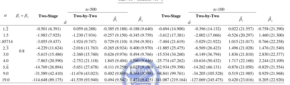
Table 2.1 summaries the result with covariates in absence of censoring. Our focus is on comparing the two methods after adjustment for the effects of β1 andβ2. The variation of

the two approaches is close. However, the two-by-two table approach seems to produce less biased estimates. Table 2.2 and 2.3 are the results in presence of right censoring. The estimators of α have larger variation but still perform well. All of the estimators are consistent when the sample size increases. In the simulations not reported here, we find that the estimators of α become invalid if the marginal heterogeneity is ignored.

Chapter 6 Conclusion

In the thesis, we review three inference approaches for estimating the association parameter for copula models. The existing methods are originally developed for analyzing homogeneous data. Here we extend these methods to account for marginal heterogeneity explained by covariates.

The two-stage estimation procedure proposed by Shih and Louis (1995) is easy to implement but not applicable under more complicated data structures such as semi-competing risks data that involves dependent censoring. The proposed approach based on two-by-two tables is motivated by the Log-Rank statistics. In comparison, it is a simple procedure from both aspects of analytic derivations and computation. It also has nice performance in simulations. Since this approach only utilizes some moment conditions, it can be easily modified for different data structures. The estimator of Hsu and Prentice (1996) has poor performance in our simulations. If our numerical algorithm is correct, the poor performance may be caused by the plugged-in estimators of the nuisance functions.

The proposed method and the method by Hsu and Prentice (1996) are both moment-based procedures but their performances are very different. We have found that, for AC models, the odds ratio of the two-by-two table provides a better descriptive measure for the association. In contrast, the covariance function of martingale residuals proposed by Hsu and Prentice is much less natural. That is why it produces an estimating function that involves many nuisance parameters.

Table 1.1 Comparison of two approaches without external censoring. ) 10 (st.error 10 bias× −2 × -2 n=500 n=100 Two-Stage Two-Stage α

parametric semi-parametric Two-by-Two Table Parametric semi-parametric Two-by-Two Table

2 1. -0.213 (8.114) 0.669 (8.382) -0.026 (8.275) 0.968 (14.767) 3.8 (16.271) 0.383 (15.232) 1.5 -0.191 (10.047) 1.179 (10.531) 0.065 (10.536) 1.464 (19.040) 6.054 (20.966) 0.28 (20.749) 1.85714 -0.252 (12.514) 1.192 (13.326) 0.031 (13.401) 2.138 (23.801) 7.592 (26.739) -0.074 (27.063) 3 2. -0.393 (15.841) 0.844 (17.039) -0.042 (17.170) 2.793 (30.204) 7.993 (33.793) -0.028 (34.737) 3.0 -0.578 (20.526) 0.018 (22.080) -0.208 (22.244) 3.637 (39.343) 7.128 (43.565) -1.11 (45.182) 4.0 -0.882 (27.588) -1.561 (29.449) -0.306 (29.807) 4.775 (53.258) 4.507 (57.379) -2.252 (60.220) 6 . 5 -1.438 (39.439) -5.398 (41.709) -0.683 (42.362) 6.37 (76.751) -2.423 (81.810) -0.963 (85.493) 9.0 -2.532 (63.241) -16.53 (65.670) -1.721 (66.599) 9.213 (123.879) -29.453 (128.361) 0.159 (136.928) 19.0 -5.370 (134.733) -72.600 (138.037) -2.178 (142.870) 16.84 (264.620) -173.33 (271.930) 9.597 (303.381)

Table 1.2 Comparison of two approaches with censoring rate 0.3. ) 10 (st.error 10 bias× −2 × -2 n=500 n=100 Two-Stage Two-Stage α

parametric semi-parametric Two-by-Two Table Parametric semi-parametric Two-by-Two Table

2 1. 0.073 (9.088) 0.566 (9.182) 0.142 (9.068) 2.061 (16.984) 4.258 (18.502) 1.702 (17.562) 1.5 0.234 (11.437) 1.024 (11.641) 0.34 (11.635) 2.747 (22.384) 5.737 (23.998) 1.252 (23.918) 1.85714 0.19 (14.198) 0.965 (14.721) 0.334 (14.909) 3.487 (27.112) 6.941 (29.197) 1.423 (30.365) 3 2. 0.024 (17.916) 0.395 (18.709) 0.244 (19.105) 4.139 (34.322) 7.02 (36.550) 1.254 (39.061) 3.0 -0.314 (22.888) -0.743 (24.042) 0.255 (24.793) 4.853 (44.807) 5.003 (47.158) 0.051 (51.647) 4.0 -1.224 (30.484) -3.377 (31.640) 0.078 (33.127) 3.853 (60.379) -2.213 (61.451) 0.297 (69.924) 6 . 5 -2.872 (43.457) -9.567 (44.718) 0.114 (47.279) 0.406 (86.207) -21.197 (83.557) 5.469 (99.999) 9.0 -9.223 (68.992) -31.33 (69.585) 0.634 (74.918) -21.92 (141.180) -88.543 (128.043) 16.75 (165.275) 19.0 -70.26 (158.490) -189.043 (152.155) 3.405 (161.384) -212.22 (348.587) -481.44 (260.105) 33.59 (369.187)

Table 1.3 Comparison of two approaches with censoring rate 0.6. ) 10 (st.error 10 bias× −2 × -2 n=500 n=100 Two-Stage Two-Stage α

parametric semi-parametric Two-by-Two Table parametric semi-parametric

Two-by-Two Table 2 1. 0.44 (10.714) 0.584 (10.759) 0.53 (10.736) 4.018 (21.149) 5.067 (22.596) 0.846 (21.655) 1.5 0.323 (13.202) 0.703 (13.357) 0.442 (13.401) 4.091 (27.924) 6.032 (29.777) 0.639 (29.280) 1.85714 0.317 (16.350) 0.685 (16.582) 0.409 (16.822) 5.072 (34.088) 7.577 (36.085) 1.563 (36.934) 3 2. 0.199 (20.272) 0.409 (20.862) 0.416 (21.371) 6.378 (42.449) 8.277 (43.924) 0.798 (46.024) 3.0 0.073 (26.114) -0.205 (27.040) 0.577 (28.097) 7.54 (54.756) 7.428 (55.933) 0.861 (60.081) 4.0 -0.299 (34.732) -1.645 (36.026) 0.928 (37.965) 7.942 (72.487) 2.874 (73.717) 2.214 (83.575) 6 . 5 -1.692 (49.035) -5.835 (50.423) 1.059 (53.934) 6.253 (104.281) -10.142 (103.610) 7.152 (119.437) 9.0 -7.103 (78.580) -19.496 (79.399) 2.336 (86.260) -6.881 (166.990) -53.666 (159.488) 25.38 (196.765) 19.0 -54.14 (175.675) -124.01 (168.489) 6.457 (184.836) -165.24 (373.784) -377.02 (315.480) 32.51 (453.817)

Table 2.1 Comparison of two approaches under marginal heterogeneity without external censoring. ) 10 (st.error 10 bias× −2 × -2 n=500 n=100

Two-Stage Two-by-Two Two-Stage Two-by-Two

α β₁ = β₂ αˆ βˆ1 βˆ2 α ˆ βˆ1 βˆ2 2 1. -0.501 (6.391) 0.059 (6.288) -0.385 (9.188) -0.188 (9.640) -0.694 (14.900) -0.396 (14.132) 0.022 (21.557) -0.758 (21.390) 1.5 -1.983 (7.925) -1.230 (7.934) -0.257 (9.150) -0.345 (9.759) -3.612 (17.381) -2.002 (17.066) -0.526 (20.297) 1.460 (21.300) 1.85714 -3.055 (9.437) -1.924 (9.747) 0.729 (9.110) 0.194 (9.501) -7.404 (21.619) -5.029 (21.922) 1.015 (21.017) 0.766 (22.258) 3 2. -4.229 (11.624) -2.016 (11.763) -0.265 (8.924) 0.400 (9.970) -11.885 (25.475) -6.569 (26.423) 1.496 (21.028) 1.476 (21.540) 3.0 -5.615 (15.486) -2.360 (15.760) 0.626 (9.976) 0.494 (9.766) -15.534 (34.260) -6.149 (36.794) 1.836 (21.810) 2.830 (22.377) 4.0 -7.863 (20.590) -2.752 (21.118) 1.845 (9.404) 1.580 (9.646) -25.774 (47.262) -10.616 (50.432) 1.717 (22.160) 2.244 (23.109) 6 . 5 -14.769 (26.894) -5.651 (27.678) -0.111 (9.259) 0.027 (9.180) -42.934 (59.398) -14.262 (66.131) -0.876 (21.050) -0.829 (21.554) 9.0 -31.589 (42.410) -11.676 (43.023) 0.402 (9.888) 0.364 (9.788) -98.841 (99.761) -34.205 (105.528) 0.519 (21.985) 0.929 (21.968) 19.0 0.8 -114.648 (89.175) -41.539 (93.940) 0.494 (9.542) 0.473 (9.435) -341.087 (219.164) -127.069 (245.475) 0.420 (23.016) 0.205 (22.920)

Table 2.2 Comparison of two approaches under marginal heterogeneity with censoring rate 0.3. ) 10 (st.error 10 bias× −2 × -2 n=500 n=100

Two-Stage Two-by-Two Two-Stage Two-by-Two

α β₁ = β₂ αˆ βˆ1 βˆ2 α ˆ βˆ1 βˆ2 2 1. -0.267 (7.589) -0.250 (8.413) -0.345 (10.011) 0.080 (10.170) 0.638 (16.577) 1.978 (18.085) -0.614 (22.271) 0.593 (23.457) 1.5 -1.858 (9.418) -1.567 (10.379) 0.083 (9.424) -0.124 (10.435) -2.140 (21.365) -1.309 (23.301) -0.466 (22.783) 1.363 (25.114) 1.85714 -1.963 (10.775) -1.007 (11.722) 0.337 (9.852) 1.079 (10.411) -4.958 (23.924) -0.703 (28.945) 0.933 (22.150) 0.658 (23.185) 3 2. -3.272 (14.306) -0.576 (16.869) 0.232 (10.123) 0.704 (10.714) -10.582 (31.164) -3.821 (36.515) -0.872 (23.256) -0.840 (24.870) 3.0 -6.165 (17.556) -1.408 (20.790) 0.327 (10.057) 0.704 (10.849) -21.709 (37.096) -10.014 (45.931) 1.367 (24.254) 1.187 (23.103) 4.0 -7.834 (23.841) 0.285 (27.205) -0.431 (11.057) -0.273 (10.434) -24.520 (52.442) 3.311 (69.246) 1.304 (24.693) 1.672 (24.308) 6 . 5 -17.583 (31.227) -1.378 (36.732) 0.574 (10.675) 0.352 (10.524) -57.033 (69.257) -2.362 (98.199) 1.592 (23.854) 1.033 (23.943) 9.0 -109.124 (55.087) -58.938 (66.582) 0.586 (10.134) 0.349 (10.517) -259.518 (111.386) -135.602 (152.304) 2.719 (23.804) 0.992 (24.344) 19.0 0.8 -292.511 (127.019) -97.013 (136.070) 0.397 (11.115) 0.562 (11.293) -668.705 (210.578) -183.206 (335.635) 2.082 (24.015) 2.155 (24.233)

Table 2.3 Comparison of two approaches under marginal heterogeneity with censoring rate 0.6. ) 10 (st.error 10 bias× −2 × -2 n=500 n=100

Two-Stage Two-by-Two Two-Stage Two-by-Two

α β₁ = β₂ αˆ βˆ1 βˆ2 α ˆ βˆ1 βˆ2 2 1. -0.022 (9.175) 0.647 (11.317) 0.480 (11.516) 0.484 (12.338) 0.535 (19.467) 5.426 (27.392) 0.403 (27.579) 1.314 (28.132) 1.5 -0.700 (11.438) 0.997 (14.396) -0.311 (11.200) 0.597 (12.072) 0.269 (27.556) 2.762 (34.610) -0.788 (25.720) 0.609 (27.642) 1.85714 -1.103 (13.657) 0.187 (16.934) -0.092 (11.824) 0.619 (11.884) -2.658 (29.413) 1.710 (39.691) 1.143 (26.587) 4.003 (29.461) 3 2. -2.726 (18.460) 0.039 (23.483) -0.025 (11.456) 0.230 (12.124) -4.620 (40.159) 5.159 (57.367) -0.679 (27.484) -0.800 (28.109) 3.0 -5.260 (21.654) -1.091 (27.524) -0.243 (11.857) 0.166 (11.525) -14.801 (51.198) -1.219 (74.896) 1.004 (28.668) 2.123 (27.966) 4.0 -13.133 (28.383) -5.477 (37.248) 0.005 (12.170) 0.090 (11.847) -34.456 (62.953) 2.777 (97.260) 1.595 (27.887) -0.243 (26.747) 6 . 5 -22.755 (42.830) -6.343 (56.938) -0.314 (11.934) 1.115 (13.131) -70.193 (94.419) -13.234 (133.771) 0.490 (27.494) 0.838 (26.873) 9.0 -70.929 (68.613) -24.824 (92.450) -0.423 (12.367) 0.509 (11.945) -196.595 (142.673) -53.852 (234.286) 0.169 (29.724) -1.050 (26.876) 19.0 0.8 -395.364 (166.251) -185.900 (228.931) 0.254 (12.735) 0.040 (12.080) -840.543 (281.685) -326.036 (561.663) 2.275 (29.854) 0.901 (28.127)

References

Clayton, D. G. (1978). A Model for Association in Bivariate Life Tables and Its Application in Epidemiological Studies of Familial Tendency in Chronic Disease Incidence. Biometrics, 65, 141-151.

Fleming, T. R. and Harrington, D. P. (1991). Counting Processes and Survival

Analysis. Wiley.

Genest, C. and Mackay, J. (1986). The Joy of Copulas: Bivariate Distributions with Uniform Marginals. The American Statistician, 40, No. 4.

Genest, C. and Rivest, L. P. (1993). Statistical Inference Procedures for Bivariate Archimedean Copulas. Journal of the American Statistical Association, 88, No. 423.

Hsu, L. and Prentice, R. L. (1996). On Assessing the Strength of Dependency Between Failure Time Variates. Biometrika, 83, 491-506.

Hsu, L. and Zhao, L. P. (1996). Assessing Familial Aggregation of Age at Onset, by Using Estimating Equations, with Application to Breast Cancer. Am. J. Hum.

Genet., 58, 1057-1071.

Nelsen, R. B. (1997). Dependence and Order in Families of Archimedean Copulas.

Journal of Multivariate Analysis, 60, 111-122.

Oakes, D. (1989). Bivariate Survival Models Induced by Frailties. Journal of the

American Statistical Association, 84, 487-493.

Prentice, R. L. and Cai, J. (1992). Covariance and Survival Function Estimation Using Censored Multivariate Failure Time Data. Biometrika, 79, 495-512.

Shih, J. H. and Louis, T. A. (1995). Inference on the Association Parameter in Copula Models for Bivariate Survival Data. Biometrics, 51, 1384-1399.

Wang, W. (2003). Estimating the Association Parameter for Copula Models under Dependent Censoring. Journal of the Royal Statistical Society: Series B, 65, 257-73.

Wei, L. J., Lin, D. Y. and Weissfeld, L. (1989). Regression Analysis of Multivariate Incomplete Failure Time Data by Modeling Marginal Distributions. Journal of

Appendix: Checking the Validity of the Method by Hsu and Prentice

Investigation #1: Is the distribution of αˆ reasonable?

Figure A.1

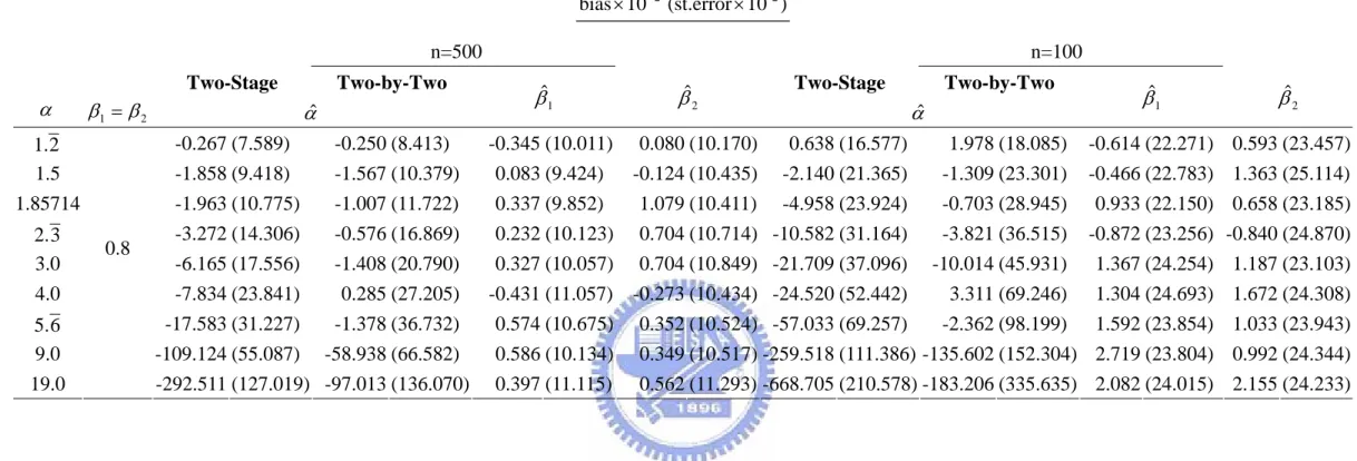
Investigation #2: Whether the above problem is caused by the root-finding procedure?

Figure A.2 plot of α = 9

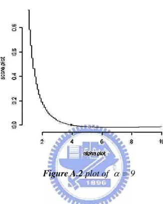
Investigation #3: Whether the plug-in estimators for the nuisance functions are not accurate?

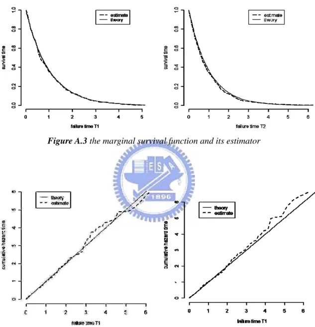
Figure A.3 the marginal survival function and its estimator

Figure A.4 the cumulative hazard function and its estimator

Finding: The plugged-in estimator have reasonable performance only in some region.