應用於3D視訊多媒體之多核心微型通訊系統研究---子計畫五：高畫質多視角立體視訊核心技術研究(I)

行政院國家科學委員會專題研究計畫 成果報告

應用於 3D 視訊多媒體之多核心微型通訊系統研究--子計畫

五：高畫質多視角立體視訊核心技術研究(I)

研究成果報告(精簡版)

計 畫 類 別 ： 整合型 計 畫 編 號 ： NSC 99-2221-E-009-185- 執 行 期 間 ： 99 年 08 月 01 日至 100 年 07 月 31 日 執 行 單 位 ： 國立交通大學電子工程學系及電子研究所 計 畫 主 持 人 ： 張添烜 計畫參與人員： 碩士班研究生-兼任助理人員：張輔仁 碩士班研究生-兼任助理人員：鄭兆傑 碩士班研究生-兼任助理人員：吳英佑 博士班研究生-兼任助理人員：李國龍 博士班研究生-兼任助理人員：陳易群 博士班研究生-兼任助理人員：曾宇晟 報 告 附 件 ： 出席國際會議研究心得報告及發表論文 處 理 方 式 ： 本計畫可公開查詢

中 華 民 國 100 年 10 月 25 日

應用於 3D 視訊多媒體之多核心微型通

訊系統研究--子計畫五：高畫質多視角立

Abstract

Nowadays, the 3D image processing has become a trend in the related visual processing field. Many automatic 2D to 3D conversion algorithms have been proposed to solve the lack of 3D content. But there is still no fast algorithm that converts single monocular images well.

In this thesis, we propose a fast conversion algorithm that includes the image segmentation, image classification, object boundary tracing method, and 3D image generation. The image segmentation adopts the watershed method to easily collect the information of depth cue. Then, the image classification recovers the geometry of scene in the image. With the depth cue and geometry information, the object boundary tracing method is proposed to detect objects in image efficiently. Finally, the object result is used to generate depth map and 3D anaglyph image.

To evaluate the results, we compare the stereo images with other 2D to 3D conversion systems. Experiment result shows that the proposed 2D to 3D conversion algorithm could perform better than the associated ones in the depth accuracy and processing speed for converting monocular images.

3

Contents

1. Report---1

1-1. Introduction---1

1-2. Target---1

1-3. Previous work---1

1-4. Proposed algorithm---2

1-4-a. Initial Segmentation---3

1-4-b. Surface layout---3

1-4-c. Object boundary tracing method---4

1-4-d. Constraint segmentation---5

1-4-e. Depth assignment and 3D image construction--5

1-5. Result---6

1-6. Conclusion---7

2. Reference---8

1

1. Report

1-1 Introduction

Video is a widely used multimedia nowadays. After the resolution of video reach a full HD(1920*1080) level, human starts to seek a more realistic way to enjoy it. Therefore, the research in 3D video has become more and more popular. However, the traditional contents are all 2D contents and they cannot fit a 3D display device. Because of the reason, many automatic 2D to 3D conversion algorithms have been proposed to solve the lack of 3D content. But there is still no fast algorithm that converts monocular still images well.

1-2 Target

Our goal is to develop an algorithm that can convert a traditional 2D content into a 3D one. In order to make our algorithm have a wide application, the target speed of the algorithm is 30fps for a HD1080(1920*1080) sequence. Furthermore, it can combine with other sub-project and build a transmission system. By the system, a 3D display technology will become a much easier task and it can also improve the application in many regions.

1-3 Previous work

Recovering 3D information from a 2D video is a basic problem in computer vision. Many depth cues can be used to extract the 3D information from a 2D video, but each cue has its own advantages and disadvantages for different conditions. Iinuma et al. [1] used the defocus cue to evaluate depth information by a single frame and the motion cue to convert the video. Cheng et al. [2] used the geometry cue and motion cue to evaluate the depth information. The simple concept and low computational complexity of those methods have enabled it to be adopted in real-time applications. However, those methods cannot perform well for a monocular still image.

Another approach is the pattern recognition-based method. In which, an image is first partitioned into many regions, and each region is categorized into several classes to be assigned depth. Based on this concept, Battiato et al. [3] classify regions into indoor, outdoor with geometric elements, and outdoor without geometric elements. Then, it uses the information collected in the classification step to estimate the depth. Even through this method could generate the high-quality result for the monocular still image, this method cannot perform well for many types of scenes. Hoiem et al. [4] also classify regions into several classes first. Then, they extract the boundary information of regions to merge small regions into objects, and further assign a

2

specific depth to each object according to its classes. This method can generate high-quality result for many types of scene, but its boundary extraction and object detection suffer from high computational complexity.

1-4. proposed algorithm

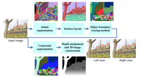
Motivated by above issues, we propose an efficient 2D to 3D conversion algorithm for monocular still images with the steps of image segmentation, image classification, object boundary tracing, constraint segmentation .and 3D image generation. First, we apply the watershed method for image segmentation, and further merge and reduce segments by texture and color information for the efficiency of successive steps. Second, we adopt the image classification [5] to recover the geometry of scene. Third, we propose the object boundary tracing method to increase the efficiency in the boundary extraction and objection detection. Fourth, we use constraint segmentation merge incomplete object segments. Finally, we assign depth for each object and synthesize a stereoscopic image by the depth-based image rendering (DIBR) algorithm [6]. The experimental results show our proposed algorithm could deliver better depth map and stereoscopic image, and speed up to 44.4 times of the previous algorithm in [4].

Initial

segmentation Surface layout

Object boundary tracing method Constraint segmentation Depth assignment and 3D image construction Right view Left view Input image

Fig. 1. Algorithm overview.

Fig.1 illustrates the flow of our 2D to 3D conversion algorithm which consists of five stages. In our method, we first use the watershed algorithm to compute the initial segmentation. Even though the watershed segmentation can preserve object boundary well, it has problems of over segmentation. Due to the problem, neighbor region merge process is used to solve this. In the second stage, we use the surface layout algorithm [5] to provide the geometric information for object detection. In the third stage, we propose the object boundary tracing method to detect object efficiently, but there are still some incomplete object segments. Thus, in the fourth stage, we perform

3

the constraint segmentation to merge segments by well-defined conditions. Finally, we assign the depths to the objects, and use the DIBR algorithm [6] to generate the images for left and right eyes in the final stage.

1-4-a. Initial Segmentation

In the proposed 2D to 3D conversion algorithm, the accuracy of object boundary detection is important. Thus a proper choice of image segmentation algorithm is also important in our approach. We adopt the watershed image segmentation [7] because it can preserve edge in the object boundary, and it is suitable for fast application.

Since the number of segments is related to the computational complexity in our algorithm, we propose a neighbor merge method to reduce the segments. In this method, we refer to the color and texture information of each small segment to further merge segments into meaningful ones.

For the color information, we consider the color distance between segments by their average color. For the color space, we apply the Hue-Saturation-Value (HSV) color space, and its color difference is computed by the formula [8]. For the texture information, we apply a subset of the filter bank in [9] to compute the texture responses of each pixel. The filter bank consists of 6 edges filters, 6 bars filters, 1 Gaussian filter, and 2 Laplacian of Gaussian filters. With the texture responses, the histogram of maximum responses is computed for every segment, and then the symmetrized Kullback-Leibler divergence is computed for every neighboring segment.

Finally, we compute the edge cost to combine the above color and texture information for every neighbor segments by the formula,

(1)

where , are the weighting factors to control the amount of color difference and divergence .

With the edge cost, two small segments could be merged if their edge cost is lower than the threshold T. The threshold is automatically and iteratively refined until the number of segment is smaller than a constant.

1-4-b Surface layout

After initial segmentation, we apply the surface layout algorithm [5] to estimate the geometry for each segment. The surface layout algorithm can label the image into geometry classes, which coarsely describe the 3D scene orientation of each image region. Every region in the image is categorized into one of three main classes: “support”, “vertical”, and “sky”. In addition, the “vertical” class is further categorized into one of five subclasses: “left”, “center”, “right”, “porous”, and “solid”. In the

4

subclasses, a planar surface facing to the “left”, “center” or “right” of the viewer, while a non-planar surface that are either “porous” or “solid”. With this algorithm, we could obtain the geometry information from an image.

1-4-c Object boundary tracing method

With above two stages, much information could help us to detect object. However, a local method is difficult to distinguish the correct boundary, while a global method has high computational complexity due to much iteration. Therefore, we propose an object boundary tracing method to solve this problem. There are three stages for the object boundary tracing method.

In the first stage, we use a set of rule to determine the initial boundaries by the features of geometry, color, texture, and boundary smoothness. With the initial boundaries selection, the obvious object boundaries are labeled.

In the second stage, we propose an efficient object boundary tracer to find the object boundary from the segmentation result in Section 2.1. In which, we starts from an initial boundary between two segments, and trace its extended boundary between another two segments. The selected boundary should have higher edge cost, high label likelihood difference between the two segments. In addition, the orientation of selected boundary cannot change rapidly. This process repeats until reaching to the border of image or the object boundary that has already been labeled.

For the proposed object boundary tracer, we defined an energy function that is formulated by the following three constraints.

Constraint 1: boundary tracing constraint:

(2) Constraint 2: different label constraint:

| ( )| (3) Constraint 3: identical label constraint:

( ( )) (4)

where i and j are the adjacent superpixels, and are the superpixel label, and is the current object label. The first one is the boundary tracing constraint to trace strong boundary. The second one is the different label constraint to separate different object. The third one is the label constraint to penalize surface label in an object.

̂ { } (5)

where , , are the weighting factors to control the amount of each energy. This cost function could be efficiently minimized by a local method.

5 1-4-d Constraint segmentation

With the proposed object boundary tracing method, some segments in the image are not complete objects. They could be further merged by the event constraints as listed in Table 1. We could merge the segments if the following conditions are satisfied.

Condition 1:

Condition 2: Condition 3: Condition 4:

We seriatim check these conditions, and merge the segments. After the constraint segmentation process, the object-based segmentation is done.

Table 1. Events of constraint segmentation

Event 1: the color of the segment is similar to the other. Event 2: the label confidence of segment is similar. Event 3: the shape of the segment is similar to the other. Event 4: the y axis position of the segment is similar Event 5: the segment is inside of the other segment. Event 6: the segment is small enough.

1-4-e Depth assignment and 3D image construction

Finally, we assign the depth to the objects according to the object segmentation result and the geometry information in Section 2.3. Our model in the 3-dimensional space consists of a ground plane and objects are orthogonal to the ground and sky.

At first, for each region, we fit a set of line segments to the ground-vertical boundary by using the Hough transform. Those line segments are used to determine that the “vertical” segments are planar or not. If a “vertical” segment contains the line segments, it is a planar. Otherwise a “vertical” segment is a non-planar.

Then, we assign different depth for segment according to their conditions. For the “ground” segment and the planar “vertical” segment, we assign gradient depth. Then, we assign corresponding depth according to the position of horizontal line and the behavior of ground-vertical boundary. For the “sky” segment and the non-planar “vertical” segment, we assign constant depth according to its position in the image coordinate.

After the depth assignment, we have the disparity map and further generate an anaglyph image for left and right eyes by the depth-based image rendering (DIBR) algorithm [6].

6 1-6. Result

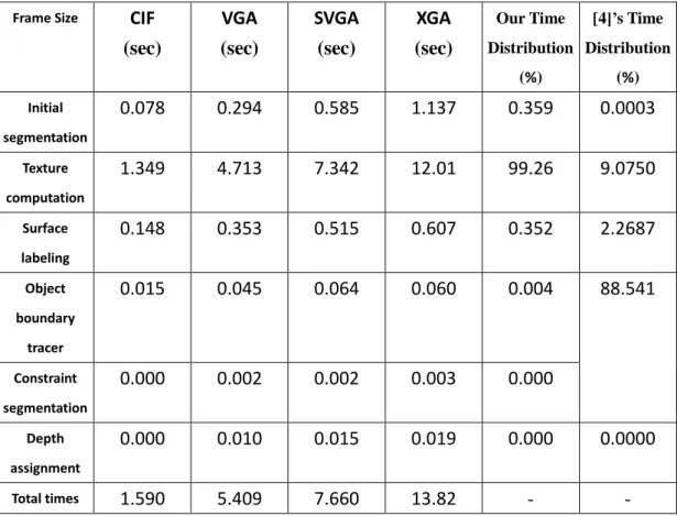
The proposed algorithm was tested on the images with the sizes from 352x288 to 1024x768, and its computation time is measured on the Intel Core i7 3.33 GHz CPU as listed in Table 2. In this table, the texture computation is bottleneck in our proposed algorithm. It is greatly increased, especially for large images. Nevertheless, the texture computation could be easily accelerated using a parallel processor. Compared to the time distribution of Hoiem’s method [4], the proposed 2D to 3D conversion algorithm could reduce the computation of object boundary tracer and constraint segmentation. Thus, our proposed algorithm is more efficient, and only needs 2.25% of the computation time in Hoiem’s method.

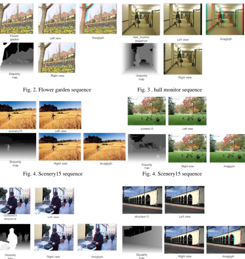
Fig. 2 to Fig. 7 show the our generated disparity maps, the left-view and right-view synthesis images, and the anaglyph images. The sequences in the Fig 2 and Fig 3 are from the standard MPEG-4 video test sequences, and the other sequences are from the databases of [4]. In the depth maps and synthesized view, our proposed algorithm could deliver better results.

Table 2. Computation time on CPU in second

Frame Size CIF

(sec) VGA (sec) SVGA (sec) XGA (sec) Our Time Distribution (%) [4]’s Time Distribution (%) Initial segmentation 0.078 0.294 0.585 1.137 0.359 0.0003 Texture computation 1.349 4.713 7.342 12.01 99.26 9.0750 Surface labeling 0.148 0.353 0.515 0.607 0.352 2.2687 Object boundary tracer 0.015 0.045 0.064 0.060 0.004 88.541 Constraint segmentation 0.000 0.002 0.002 0.003 0.000 Depth assignment 0.000 0.010 0.015 0.019 0.000 0.0000 Total times 1.590 5.409 7.660 13.82 - -

7

Fig. 2. Flower garden sequence Fig. 3 . hall monitor sequence

Fig. 4. Scenery15 sequence Fig. 4. Scenery15 sequence

Fig. 6. Outdoor21 sequence Fig. 7 . Structure10 sequence

1-7. Conclusion

In this paper, we proposed an efficient 2D to 3D conversion algorithm which automatically converts a still 2D image into a 3D one. With the proposed object boundary tracing method, the computation time is much reduced to 2.25%. The

8

proposed 2D to 3D conversion algorithm could deliver better depth map and stereoscopic images, compared to the typical algorithm.

This project has already proposed as a paper in CVGIP, 2011. The paper’s name is as follow:

Yi-Chun Chen et. al. “Efficient 2D to 3D conversion with Object-Based Segmentation”, Computer Vision, Graphics, and Image Processing (CVGIP), 2011

2. Reference

[1] T. Iinuma, H. Murata, S. Yamashita, and K. Oyamada, “Natural stereo depth creation methodology for a real-time 2D-to-3D image conversion,” SID Symposium Digest of

Technical Papers, pp. 1212-1215, 2000.

[2] C. C. Cheng, T. L. Chung, Y. M. Ysai, and L. G. Chen, “Hybrid depth cueing for 2D-to-3D conversion system,” in Proc. of Stereoscopic Displays and Application XX, 2009 [3] S. Battiato, A. Capra, S. Curti, and M. L. Cascia, "3D stereoscopic image pairs by depth-map generation," in Proc. of International Symposium on 3D Data Processing,

Visualization and Transmission (3DPVT), pp. 124-131, 2004.

[4] D. Hoiem, A. Stein, A. A. Efros, and M. Hebert, “Recovering occlusion boundaries from a single image,” in Proc. of IEEE International Conference on Computer Vision (ICCV), 2007. [5] D. Hoiem, A. Efros, and M. Hebert, “Recovering surface layout from an image,”

International Journal of Computer Vision (IJCV), vol. 75, no. 1, pp. 151–172, 2007.

[6] Y. R. Horng, Y. C. Tseng, T. S. Chang, “Stereoscopic images generation with directional Gaussian filter,” in Proc. of IEEE International Symposium on Circuits and Systems, pp. 2650-2653, 2010.

[7] A. Körbes, R. Lotufo, G. B. Vitor, and J. V. Ferreira, “A proposal for a parallel watershed transform algorithm for real-time segmentation,” in Proc. of Workshop de Vis 𝑎̃ o

Computacional, 2009.

[8] J. R. Smith and S. F. Chang, "VisualSEEk: A fully automated content-based image query system", in Proc. of ACM Multimedia Conference, pp. 87 - 98, 1996.

[9] T. Leung and J. Malik, “Representing and recognizing the visual appearance of materials using threedimensional textons,” International Journal of Computer Vision (IJCV), vol. 43, no. 1, pp. 29–44, 2001.

9

3. Self-assessment

We successfully proposed a high speed algorithm compared to other object-based ones. Under object-based algorithm, we can make a complete object in the same depth. That is, we will feel that every part in the object is at the same distance with us. It is very important for a comfortable 3D experience.

This algorithm was also published in CVGIP, 2011 as an oral paper. It will be a good reference for someone who expects to do further research in this area.

However, this algorithm cannot reach our final goal – the real time application. Although we believe that the parallel computation can speed up the algorithm a lot, it may not reach 30fps when handling a full HD sequence. For a realistic application, we should try to simplify and speed up this algorithm.

The other question is that there is no standard for evaluating the qualities of 2D to 3D conversion algorithm since there is no ground truth for a real 2D sequence. Furthermore, the confortable 3D content is a complex issue because it will depend on human’s feeling. The judgment way should be different from the traditional 2D sequence. We believe that to establish a fair computation method to judge which algorithm is better will be an important issue in the related research.

 Published paper

Yi-Chun Chen et. al. “Efficient 2D to 3D conversion with Object-Based Segmentation”, Computer Vision, Graphics, and Image Processing (CVGIP), 2011

1

國科會補助專題研究計畫項下出席國際學術會議心得報告

日期： 100 年 8 月 2 日

一、參加會議經過

7 月 6 日抵達希臘科孚島。參加 SESSION W1C Image Sequence and Stereoscopic

Processing，此場次有兩篇實驗室的論文發表。接下來下午各別參加了兩場 SESSION

W3A Human 3D Perception and 3D Video Assessments 以及 W2B Architecture and

Implementations I。晚上參加 Welcome Reception.

7 月 7 日早上參加 SESSION T1C Image and Video Coding I 並發表論文。接下來參

加了

SESSION T2B Signal Processing for Communications II 並聽了幾篇論文報告。中

午用完餐後，參加了下午的

Plenary 3: Binaural Signal Processing。接下來又參加了兩

場

SESSION T3A Signal and Image Restoration 以及 SESSION T4B Image Processing

Applications。

由於我們國內班機是

7 月 8 日下午，所以早上只去參加了一個 SESSION F1C Image

and Video Coding II 之後就回飯店整理行李去搭機了。

計畫編號

NSC 99-2221-E-009-185

計畫名稱

應用於

3D 視訊多媒體之多核心微型通訊系統研究--子計畫五：高畫質

多視角立體視訊核心技術研究(I)

出國人員

姓名

李國龍

服務機構

及職稱

交通大學電子工程系所

會議時間

100 年 7 月 6 日至

100 年 7 月 8 日

會議地點

科孚島(Corfu),希臘( Greece)

會議名稱

(中文)第 17 屆國際電子電機學會數位訊號處理國際研討會

(英文)17th IEEE International Conference on Digital Signal Processing

發表論文

題目

(中文) 一個適用於 H.264/AVC 可調式視訊編碼分數點移動估測之有

效率模式預先選擇演算法

( 英 文 )An Efficient Mode Pre-Selection Algorithm for H.264/AVC

Scalable Video Extension Fractional Motion Estimation

2

二、與會心得

此會議為訊號處理領域的主要會議，其中包含了通訊、語音編碼、視訊編碼、影

像處理以及與數位訊號相關之議題。在此會議中，參加了數場發表場次，也聽了不

少篇國外學者所做的研究。雖然說這個會議選擇在希臘的一個離島舉辦，原本預期

心理會覺得應該論文數量不多且論文品質可能不高，但是，聽了這幾場之後，我發

現此會議所接受的論文品質似乎具有一定的水準。所以，參加此會議讓我又多了解

了許多數位訊號處理研究議題。

三、考察參觀活動(無是項活動者略)

略

四、建議

此會議雖然規模小，但卻是五臟俱全。然而，由於參加會議那段時間剛好是希臘

罷工潮，所以遇到罷工事件導致科孚島上所有計程車在我們抵達那天皆沒有營運。

更慘的事是，主辦單位也沒有查覺這件事，最後導致我們拖著行李徒步至開會飯店。

因此，建議如果以後遇到國內有罷工事件的話，那麼主辦單位最好是安排公車讓參

與者搭乘。

五、攜回資料名稱及內容

研討會會議手冊(內含會議行程以及詳細各場次所欲發表之論文題目)

會議光碟(內含所有完整會議資訊以及所有論文全文)

六、其他

無

DSP2011 notification for paper 115

2 封郵件 Gwo-Long Li <[email protected]> DSP2011 <[email protected]> 2011年3月26日上午6:01 收件者: Gwo-Long Li <[email protected]> Dear Author(s),

Thank you for submitting your manuscript to the 17th International Conference on Digital Signal

Processing (DSP2011). The review process has now been concluded and it is our pleasure to inform you that your proposed paper 115 entitled

AN EFFICIENT FRACTIONAL MOTION ESTIMATION MODE SELECTION ALGORITHM FOR H.264/AVC SCALABLE VIDEO EXTENSION

has been ACCEPTED for publication.

The reviews for your paper are attached below. They served as the basis for the Technical Program Committee's decision. Please make sure that you＇ll incorporate all the reviewers＇ suggestions and comments during the preparation of your camera-ready paper. In the next days you will receive additional information regarding your camera ready manuscript submission procedure and deadline.

Please note that for each accepted paper, it is required that at least one author registers (at full rate) for the conference before May 1st, 2011. Papers that are not registered by this deadline will not be

included in the proceedings and in the final program. Registration instructions will be sent to you soon.

Thank you for submitting your paper to DSP2011. Looking forward to welcoming you to Corfu in July!

Best regards,

The DSP2011 Technical Program Chairs Andreas Floros, Ionian University, Greece Giovanni Poggi, University of Naples, Italy

--- REVIEW 1 --- PAPER: 115

TITLE: AN EFFICIENT FRACTIONAL MOTION ESTIMATION MODE SELECTION ALGORITHM FOR H.264/AVC SCALABLE VIDEO EXTENSION

AUTHORS: Gwo-Long Li and Tian-Sheuan Chang

OVERALL RATING: 1 (weak accept) NOVELTY AND ORIGINALITY: 4 (good)

TECHNICAL CONTENT AND CORRECTNESS: 4 (good) CLARITY OF PRESENTATION: 4 (good)

RELEVANCE TO THE CONFERENCE: 3 (fair)

For what motion estimation technique are the memory bandwidth requirements reported in sec. 2.1?

The bit rate differences in Fig 4 and 5 should be given in relative numbers (bit rate increase in percent) instead of absolute numbers (bit rate increase in kbps).

Page 1 of 2 Gmail - DSP2011 notification for paper 115

2011-08-02 https://mail.google.com/mail/?ui=2&ik=b51218734b&view=pt&cat=Paper%20Submissi...

It should be further discussed how the effectiveness of the proposed technique depends on the employed motion estimation strategy.

I would further suggest to add rate distortion curves (instead of the PSNR and bit rate difference curves) in order to illustrate the impact on the rate distortion efficiency.

--- REVIEW 2 --- PAPER: 115

TITLE: AN EFFICIENT FRACTIONAL MOTION ESTIMATION MODE SELECTION ALGORITHM FOR H.264/AVC SCALABLE VIDEO EXTENSION

AUTHORS: Gwo-Long Li and Tian-Sheuan Chang

OVERALL RATING: 1 (weak accept) NOVELTY AND ORIGINALITY: 3 (fair)

TECHNICAL CONTENT AND CORRECTNESS: 3 (fair) CLARITY OF PRESENTATION: 4 (good)

RELEVANCE TO THE CONFERENCE: 5 (excellent)

Fast mode decision algorithms have been in use for H.264. What is new in this paper for SVC is a way to avoid the fractional pel motion estimation for the new SVC modes - motion prediction, residual prediction.

The proposed method looks at integer pel cost to avoid some of the fractional pel cost

computations. While the basic concept is not new, it may be new when applied in the SVC concept. Hence the rating for "innovation" and "technical content" are given as average.

Some of the experimental results are surely useful for the SVC comminity - hence the relevance is given as "excellent" - and seing from the CFP fo the conference, teh contents seem to fit in.

Points for potential improvement:

1. Some gramatical mistakes could have been avoided.

2. The introduction directly jumps to an existing fast ME / mode decision algorithm without even a paragraph of background to SVC, and what is currently available for SVC in public implementations.

Gwo-Long Li <[email protected]> 2011年3月28日上午11:13

收件者: [email protected]

[隱藏引用文字]

Page 2 of 2 Gmail - DSP2011 notification for paper 115

2011-08-02 https://mail.google.com/mail/?ui=2&ik=b51218734b&view=pt&cat=Paper%20Submissi...

AN EFFICIENT MODE PRE-SELECTION ALGORITHM FOR H.264/AVC SCALABLE VIDEO EXTENSION FRACTIONAL MOTION ESTIMATION

Gwo-Long Li and Tian-Sheuan Chang

Department of Electronics Engineering & Institute of Electronics National Chiao Tung University

ABSTRACT

H.264/AVC scalable video extension (SVC) adopts various advanced prediction modes to exploit the data redundancies between layers for better coding efficiency but at the cost of significantly increased computational complexity, especially for hardware realization of fractional motion estimation. This paper proposes an efficient and hardware friendly mode pre-selection algorithm which only preserves the possible prediction modes for fractional motion estimation through the pre-selection rules proposed in this paper. Simulation results demonstrate that our proposed algorithm can reduce up to 72.92% prediction modes with only 1.24% bitrate increase and 0.02dB PSNR degradation.

Index Terms— Fractional motion estimation, Mode

pre-selection, Inter-layer prediction, H.264/AVC Scalable Extension

1. INTRODUCTION

Fractional motion estimation (FME) is one of the commonly adopted techniques in video coding system to further improve the rate distortion performance [1]. The operation of FME is mainly composed by two stages called half-pixel stage and quarter-pixel stage and each stage executes search and interpolation process to find out the best prediction results. Although FME only checks several positions around the best motion vectors produced by integer motion estimation (IME), the computational complexity of IME and FME are almost equal to each other especially in hardware realization due to the complicated interpolation process and a lot of prediction modes need to be checked by FME [2]. As a result, the operations of IME and FME are usually divided into two different pipeline stages in hardware design [3] to aim at higher coding performance.

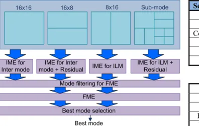
In H.264 video coding standard [1], seven block sizes are supported in inter prediction mode and each partition size has to be checked by IME and FME one by one to select the best prediction result as shown in Fig.1. Thus, 41 blocks have to go through IME and FME operation. In addition to the inherent prediction modes in H.264, the mechanism of inter-layer prediction adopted in SVC [4] significantly increases the computational complexity of FME as shown in Fig.2, including inter-layer motion prediction (ILM), and

inter-layer motion residual prediction (ILM+R). As a result, 41×4=164 blocks have to be examined by FME in SVC.

To simplify the design complexity in hardware realization, the small blocks ranged from 8×8 to 4×4 are early decided in IME stage to derive a Sub-mode and thus only partition sizes of 16×16, 16×8, 8×16, and Sub-mode (9 blocks in minimum and 21 blocks in maximum) have to be examined by FME operation as Fig.3(a) shown. Similarly, the idea of Sub-mode early decision can be also applied to SVC for easing the overhead of hardware implementation. As a result, only 36 to 84 blocks have to be examined by FME for SVC as shown in Fig.4. Although the early decision method for Sub-mode can efficiently reduce the overheads of FME, the computational complexity of FME is still high. Several works [5-8] have been proposed to increase the coding speed of FME in hardware implementation. In contrast to check all prediction modes, [9,10] proposed a mode pre-selection method as shown in Fig.3(b) to pre-selecting the potential skippable prediction modes before entering FME prediction process in H.264. However, none of above literature has addressed the issues of SVC. Thus, this paper proposes an efficient mode pre-selection algorithm to lighten the computational complexity of FME for SVC through the statistical observations.

The rests of this paper are organized as follows. In Section 2, some observations are introduced to indicate the rate distortion cost relationship between different prediction modes. Afterwards, the mode pre-selection algorithm is proposed according to the observations. Simulation results are shown in Section 3 to demonstrate the efficiency of our proposed algorithms. The conclusions are made in Section 4.

16x16 16x8 8x16 8x8

IME for Inter mode FME for Inter mode Best mode selection

Best mode

8x4

4x8 4x4

16x16 16x8 8x16 8x8 8x4 4x8 4x4 IME for Inter mode FME for Inter mode

IME for Inter mode + Residual

FME for Inter mode + Residual

IME for ILM FME for ILM

IME for ILM + Residual FME for ILM +

Residual Best mode selection

Best mode

Fig.2 Illustration of mode selection process of SVC 16x16 16x8 8x16 Sub-mode

IME for Inter mode FME for Inter mode Best mode selection

Best mode

Fig.3(a) Illustration of mode selection process for H.264

16x16 16x8 8x16 Sub-mode

IME for Inter mode Mode filtering for FME

Best mode selection Best mode

FME

Fig.3(b) Illustration of mode pre-selection concept for

H.264

IME for Inter mode

FME for Inter mode

IME for Inter mode + Residual

FME for Inter mode + Residual

IME for ILM

FME for ILM

IME for ILM + Residual FME for ILM +

Residual Best mode selection

Best mode

16x16 16x8 8x16 Sub-mode

Fig.4 Illustration of mode selection process for SVC 2. PROPOSED MODE PRE-SELCTION ALGORITHM In this section, we conduct several analyses to observe the relationship between the rate distortion costs (RDCosts) of

IME and FME of different prediction modes.

2.1. Analysis for Inter-layer and Inter prediction modes Fig. 5 shows the relationship between RDCosts of IME and

FME of different prediction modes. In this figure, the

vertical axis indicates the RDCosts and the horizontal axis is the index of macroblocks. The InterI and ILMI individually stand for the IME RDCosts of Inter and ILM mode; the

InterF and ILMF are the FME RDCosts of Inter and ILM

mode, respectively. From this figure, we can derive a property that the RDCosts of IME and FME are very close to each other for the same prediction mode. For example,

the RDCost of IME is very close to the RDCost of FME for

Inter mode and the same situation can be seen from ILM

prediction mode. Therefore, if the IME RDCost of Inter mode is sufficiently larger than that of IME RDCost of ILM mode, the FME RDCost of Inter mode will be larger than

FME RDCost of ILM mode and vice versa. As a result, we

conduct several simulations to confirm the property that we observed and the statistical results are shown in Table 1. In this table, the conditional probability of P(A|E) is defined as follows. (1) where P(E) = P(I (2) P(A)=P(In (3) (4) From the statistical results shown in Table 1, we can observe that the conditional probability of Eq.(1) could achieve up to 85.74% on average. In summary, we conclude that if IME RDCost of Inter (ILM) mode is sufficiently larger than that of IME RDCost of ILM (Inter) mode, the

FME of Inter (ILM) mode can be skipped.

(a)

(b)

Fig.5 Relationship between RDCosts of IME and FME of different prediction modes (a) Football, (b) Foreman sequence

2.2. Analysis for partition size

We further analyze the relationship between RDCosts of

IME and FME in different partition size. Four cases listed in

Eq.(5) to Eq.(8) are used to produce the analytic results shown in Table 2. From this table, if IME RDCost of 16×16 is less than IME RDCost of 16×8 or 8×16, more than 95.83% of probability that FME RDCost of 16×16 will less than FME RDCost of 16×8 or 8×16. Therefore, we can further filter off some modes before FME by using the observed results. (5) (6) (7) (8) 2.3. Proposed Algorithm

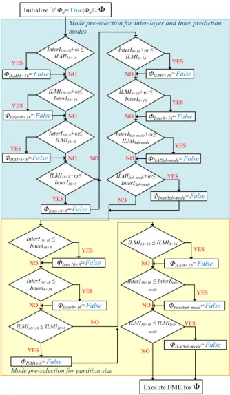
Fig.6 reveals the proposed FME mode pre-selection concept and Fig.7 shows the flowchart of our proposed mode pre-selection algorithm in which the candidate set of prediction modes Φ is defined as follows.

(9) In this flowchart, all pre-selection rules derived from previous sections are classified into two parts. The upper part is derived from the observation of the relationship between Inter and ILM predictions. The bottom part is obtained from the observation of the relationship between different partition sizes. A macroblock after IME operation will go through all determination process to filter out the potentially skippable prediction modes.

IME for Inter mode

Mode filtering for FME IME for Inter

mode + Residual IME for ILM

IME for ILM + Residual

Best mode selection Best mode

16x16 16x8 8x16 Sub-mode

FME

Fig.6 Illustration of mode FME mode pre-selection for SVC

3. SIMULATION RESULTS

In this section, several simulation results are shown to demonstrate the performance of our proposed FME mode pre-selection algorithm. The simulation settings are summarized in Table 3 and 12 test sequences including various motion activities are used to produce the simulation results. Table 4 shows the bit rate comparison of our proposed algorithm with JSVM9.17[11]. From this table, the bit rate increasing of our proposed algorithm is only 1.24% on average. For PSNR comparison as shown in Table 5, our proposed algorithm only conducts 0.02dB PSNR degradation on average when compared to JSVM. The percentage of mode reduction of our proposed algorithm is listed in Table 6. Our proposed algorithm can achieve 72.92% mode reductions when compared to JSVM on average. For the high motion sequences such as Stefan, Soccer and Football, we can observe that the mode reductions are much higher than slow and median motion sequences. This situation is because that RDCost difference between two modes in high motion sequences is much larger than RDCost difference between two modes in slow motion sequences. Therefore, it is easy to distinguish the skippable modes by our proposed mode pre-selection rules listed in Eq.(1) to Eq.(4). Similarity, since RDCost difference between two modes in slow motion sequences is marginal, less prediction modes could be skipped by our proposed mode pre-selection algorithm.

Table 1. Statistical results of Eq.(1)

Sequences P(A|E)×100% Sequences P(A|E)×100% Akiyo 97.81 Tempete 83.52 Dancer 96.71 Football 83.62 Coastguard 78.53 Foreman 81.59 Table 85.51 M&D 97.26 Mobile 70.61 Soccer 80.11 News 97.37 Stefan 76.25

Table 2. RDCost relationship between partition sizes Sequences P(A|E)×100% Sequences P(A|E)×100%

Akiyo 99.31% Tempete 91.77% Dancer 98.80% Football 92.74% Coastguard 97.03% Foreman 97.61% Table 97.62% M&D 99.53% Mobile 88.12% Soccer 98.12% News 98.79% Stefan 90.54%

Table 3. Simulation settings

Reference software JSVM9.17 [11] QP for spatial base layer 38 QP for Spatial enh. layer 32 Frame size in spatial base layer QCIF

Frame size in spatial enh. ayer CIF Frames to be encoded 150

Table 4. Bitrate comparison of proposed algorithm JSVM Proposed Increasing (%) Akiyo 29.23 29.72 1.69 % Dancer 117.11 118.58 1.26 % Coastguard 264.93 267.03 0.79 % Table 181.62 184.12 1.38 % Tempete 225.52 227.77 1.00 % Football 332.05 335.79 1.13 % Foreman 111.12 113.16 1.84 % MD 45.89 46.79 1.96 % Mobile 338.48 341.41 0.86 % News 68.92 69.66 1.07 % Soccer 186.04 187.56 0.82 % Stefan 284.97 287.91 1.03 % Table 5. PSNR comparison of proposed algorithm

JSVM Proposed Difference (dB) Akiyo 39.94 39.92 -0.02 Dancer 41.00 41.00 -0.00 Coastguard 33.97 33.96 -0.01 Table 35.33 35.31 -0.02 Tempete 34.37 34.35 -0.02 Football 35.69 35.68 -0.01 Foreman 36.69 36.68 -0.01 MD 38.95 38.91 -0.04 Mobile 33.51 33.49 -0.02 News 38.24 38.22 -0.01 Soccer 35.77 35.74 -0.03 Stefan 34.85 34.84 -0.01 Table 6 Averaged mode reduction of our proposal (Unit: %)

Akiyo Dancer Coastguard Table Tempete MD 62.50 68.75 75.00 75.00 75.00 68.75 Football Mobile Foreman News Stefan Soccer

81.25 75.00 75.00 68.75 75.00 75.00 4. CONCLUSION

In this paper, an efficient mode pre-selection algorithm for fraction motion estimation is proposed to reduce the computational complexity of fraction motion estimation in SVC. By observing the relationship between IME RDCosts and FME RDCosts of different prediction modes, several mode pre-selection rules are proposed to reject some potentially skippable modes before FME operation. In addition, since our proposed mode pre-selection algorithm is only composed by several simple additions, subtractions, and comparators, it can be easily realized in hardware form. Simulation results demonstrate that our proposed algorithm can reduce 72.92% prediction modes on average before entering FME operation. In addition, the bitrate increasing and PSNR degradation of our proposed algorithm is only 1.24% and 0.02dB, respectively.

5. ACKNOWLEDGE

This work was supported by National Science Council of Taiwan, under Grant NSC98-2220-E-009-001.

Initialize ∀Φij=True|Φij∈Φ InterI16× 16+ω ≤ ILMI16× 16 ILMI16× 16+ω≤ InterI16× 16 InterI16× 8+ω≤ ILMI16× 8 ILMI16× 8+ω≤ InterI16× 8 InterI8× 16+ω ≤ ILMI8× 16 ILMI8× 16+ω ≤ InterI8× 16 InterISub-mode+ω≤ ILMISub-mode ILMISub-mode+ω≤ InterISub-mode ΦILM16× 16=False ΦInter16× 16=False ΦInter16× 8=False ΦILM16× 8=False ΦILM8× 16=False ΦInter8× 16=False ΦILMSub-mode=False YES YES YES YES YES YES YES NO NO NO NO NO NO NO InterI16× 16 ≤ InterI16× 8 InterI16× 16 ≤ InterI8× 16 ILMI16× 16 ≤ ILMI16× 8 ILMI16× 16 ≤ ILMI8× 16 ΦInter16× 8=False ΦInter8× 16=False ΦILM16×8=False YES YES NO NO ΦInterSub-mode=False YES

InterI16× 16 ≤ InterI Sub-mode

ILMI16× 16 ≤ ILMI Sub-mode ΦInterSub-mode=False YES NO NO ΦILMSub-mode=False YES NO ΦILM8× 16=False YES NO

Execute FME for Φ

NO

Mode pre-selection for Inter-layer and Inter prediction modes

Mode pre-selection for partition size

YES

Fig.7 Flowchart of our proposed FME mode pre-selection algorithm

6. REFERENCES

[1] Draft ITU-T Recommendation and Final Draft International Standard of Joint Video Specification (ITU-T Rec. H.264/ISO/IEC14496-10 AVC), March 2003.

[2] T.-C. Wang, Y.-W. Huang, H.-C. Fang, L.-G. Chen, “Performance analysis of hardware oriented algorithm modifications in H.264,” in proceeding of IEEE International Conference on Acoustics, Speech, and Signal Processing, vol.2, pp.493-496, April 2003.

[3] Y.-K. Lin, D.-W. Li, C.-C. Lin, T.-Y. Kuo, S.-J. Wu, W.-C. Tai, W.-C. Chang, and T.-S. Chang, ” A 242mW, 10mm2 1080p H.264/AVC High Profile Encoder Chip,” in proceeding of International Solid-State Circuits Conference (ISSCC), pp. 314-315, Feb. 2008.

[4] H. Schwarz, D. Marpe, and T. Wiegand, “Overview of the scalable video coding extension of the H.264/AVC standard,”

IEEE Transaction on Circuits and Systems for Video Technology, vol. 17, no. 9, pp. 1103-1120, September 2007.

[5] H. Nisar and T.-S. Choi, “Fast and efficient fractional pixel motion estimation for H.264/AVC video coding,” in proceeding of IEEE International Conference on Image Processing, pp.1561-1564, 2008.

[6] C.-Y. Kao, C.-L. Wu, and Y.-L. Lin, “A High-Performance Three-Engine Architecture for H.264/AVC Fractional Motion Estimation,” IEEE Transactions on Very Large Scale Integration System, vol. 18, no. 4, pp.662-666, April 2010

[7] Y.-J. Wang, C.-C. Cheng, and T.-S. Chang, “A fast algorithm and its VLSI architecture for fractional motion estimation for H.264/MPEG-4/AVC video coding,” IEEE Transactions on Circuits and Systems for Video Technology, vol. 17, no. 5, pp. 578–583, May 2007.

[8] G. Kim, J. Kim, C.-M. Kyung, “A Low cost single-pass fractional motion estimation architecture using bit clipping for H.264 video codec,” in Proceeding of IEEE International Conference on Multimedia and Expo. pp.661-662, 2010.

[9] C.-C. Yang, K.-J. Tan, Y.-C. Yang and J.-I. Guo, “Low complexity fractional motion estimation with adaptive mode selection for H.264/AVC, in Proceeding of IEEE International Conference on Multimedia and Expo. pp.673-678, 2010.

[10] C.-C. Lin, Y.-K. Lin, and T.-S. Chang, “A fast algorithm and its architecture for motion estimation in MPEG-4 AVC/H.264,” in proceedings of Asia Pacific Conference on Circuits and Systems, pp.1250-1253, December 2006.

[11] ITU-T and I. JTC1. (2008) JSVM Software version JSVM 9.17.

國科會補助計畫衍生研發成果推廣資料表

日期:2011/10/15

國科會補助計畫

計畫名稱: 子計畫五：高畫質多視角立體視訊核心技術研究(I) 計畫主持人: 張添烜 計畫編號: 99-2221-E-009-185- 學門領域: 積體電路及系統設計

無研發成果推廣資料

99 年度專題研究計畫研究成果彙整表

計畫主持人：張添烜 計畫編號：99-2221-E-009-185- 計畫名稱：應用於 3D 視訊多媒體之多核心微型通訊系統研究--子計畫五：高畫質多視角立體視訊核心 技術研究(I) 量化 成果項目 實際已達成 數（被接受 或已發表） 預期總達成 數(含實際已 達成數) 本計畫實 際貢獻百 分比 單位 備 註 （ 質 化 說 明：如 數 個 計 畫 共 同 成 果、成 果 列 為 該 期 刊 之 封 面 故 事 ... 等） 期刊論文 0 0 100% 研究報告/技術報告 0 0 100% 研討會論文 1 1 100% 篇 論文著作 專書 0 0 100% 申請中件數 0 0 100% 專利 已獲得件數 0 0 100% 件 件數 0 0 100% 件 技術移轉 權利金 0 0 100% 千元 碩士生 0 0 100% 博士生 0 0 100% 博士後研究員 0 0 100% 國內 參與計畫人力 （本國籍） 專任助理 0 0 100% 人次 期刊論文 0 0 100% 研究報告/技術報告 0 0 100% 研討會論文 0 0 100% 篇 論文著作 專書 0 0 100% 章/本 申請中件數 0 0 100% 專利 已獲得件數 0 0 100% 件 件數 0 0 100% 件 技術移轉 權利金 0 0 100% 千元 碩士生 3 3 100% 博士生 3 3 100% 博士後研究員 0 0 100% 國外 參與計畫人力 （外國籍） 專任助理 0 0 100% 人次

其他成果

(

無法以量化表達之成 果如辦理學術活動、獲 得獎項、重要國際合 作、研究成果國際影響 力及其他協助產業技 術發展之具體效益事 項等，請以文字敘述填 列。) 無 成果項目 量化 名稱或內容性質簡述 測驗工具(含質性與量性) 0 課程/模組 0 電腦及網路系統或工具 0 教材 0 舉辦之活動/競賽 0 研討會/工作坊 0 電子報、網站 0 科 教 處 計 畫 加 填 項 目 計畫成果推廣之參與（閱聽）人數 0

國科會補助專題研究計畫成果報告自評表

請就研究內容與原計畫相符程度、達成預期目標情況、研究成果之學術或應用價

值（簡要敘述成果所代表之意義、價值、影響或進一步發展之可能性）

、是否適

合在學術期刊發表或申請專利、主要發現或其他有關價值等，作一綜合評估。

1. 請就研究內容與原計畫相符程度、達成預期目標情況作一綜合評估

■達成目標

□未達成目標（請說明，以 100 字為限）

□實驗失敗

□因故實驗中斷

□其他原因

說明：

2. 研究成果在學術期刊發表或申請專利等情形：

論文：■已發表 □未發表之文稿 □撰寫中 □無

專利：□已獲得 □申請中 ■無

技轉：□已技轉 □洽談中 ■無

其他：（以 100 字為限）

3. 請依學術成就、技術創新、社會影響等方面，評估研究成果之學術或應用價

值（簡要敘述成果所代表之意義、價值、影響或進一步發展之可能性）（以

500 字為限）

1. 學術成就: 完成現有針對單視點視訊的深度估測引擎演算法的效果分析 2. 技術創新: 3. 社會影響: