利用架設在視訊監控車上成對的全方位攝影裝置作週遭環境監控之研究

(1)

國立交通大學

資訊科學與工程研究所

碩士論文

利用架設在視訊監控車上成對的

全方位攝影裝置作週遭環境監控之研究

A Study on Surrounding Environment Monitoring by a Video

Surveillance Car with Two 2-camera Omni-imaging Devices

研究生：陳俊甫

指導教授：蔡文祥教授

(2)

利用架設在視訊監控車上成對的

全方位攝影裝置作週遭環境監控之研究

A Study on Surrounding Environment Monitoring by a Video

Surveillance Car with Two 2-camera Omni-imaging Devices

研究生：陳俊甫 Student：Chun-Fu Chen

指導教授：蔡文祥 Advisor：Wen-Hsiang Tsai

國立交通大學

多媒體工程研究所

碩士論文

A Thesis

Submitted to Institute of Multimedia Engineering College of Computer Science

National Chiao Tung University in partial Fulfillment of the Requirements

for the Degree of Master

in

Computer Science

June 2011

Hsinchu, Taiwan, Republic of China

(3)

利用架設在視訊監控車上成對的

全方位攝影裝置作週遭環境監控之研究

研究生: 陳俊甫

指導教授:蔡文祥博士

國立交通大學資訊科學與工程研究所

摘要

本研究利用架設在一視訊監控車頂上的兩組全方位攝影裝置來達到視訊監控的功能，主要應用於監控行車視角的盲點和周遭的車輛。在本研究中，此二全方位攝影機裝置可用以監看車輛周遭任何角度的影像畫面。此外，本研究利用光流分析法直接套用在連續擷取的影像上，並利用影像的移動向量分析目前車輛的行走方向，產生對應方位的透視影像(perspective-view image)，方便駕駛觀看。另一方面，本研究亦提出一種「透視對應表」(perspective mapping table)，可以快速地將全方位影像轉成透視影像，提供駕駛觀看行車紀錄。同時，本研究利用全方位攝影系統所拍攝的影像，可靜態監控周遭靜止的車輛並求得立體資訊。另利用影像處理技術取出影像中的車體區域，並偵測車窗底緣的對應點，計算車輛位置，進而產生監控車週遭環境的俯視圖。除了偵測靜態的車輛，本研究也提出了行駛當中的視訊監控車偵測到停止或移動的周遭車輛的方法。另亦使用光流分析法，配合全方位攝影機所擷取到的連續影像，利用有高度的物體會產生較大移動向量的性質，將車體給大致分割出來，進而使用「k 均值分群法」(k-means clustering)去偵測出車體，接著透過區域增長法去找出較完整的車體，最後再利用預先造好的車輛模型去做比對，藉以取得周遭車輛的位置資訊，劃出車輛周遭的俯視圖，供車輛駕駛觀看。上述方法的實驗結果皆甚良好，顯示所提視訊監控系統確實可行。

(4)

A Study on Surrounding Environment Monitoring

by a Video Surveillance Car with Two 2-camera

Omni-imaging Devices

Student: Chun-Fu Chen

Advisor: Prof. Wen-Hsiang Tsai

Institute of Multimedia Engineering, College of Computer Science

National Chiao Tung University

ABSTRACT

In this study, methods are proposed for video surveillance by a video surveillance vehicle equipped with a pair of two-camera omni-imaging devices on its roof, with emphasis on monitoring of blind spots and nearby cars around the vehicle.

First, for generating perspective-view images to facilitate inspection of the vehicle’s surrounding environment, a space-mapping table and an r- mapping table are created to accelerate the related coordinate transformation process. Also, a method for generating the perspective-view image of the surrounding area of the vehicle by estimating the vehicle’s moving direction using optical flow analysis is proposed. For off-line inspection of the driving history, a method of using a perspective-mapping table proposed in this study to generate a series of perspective-view images of any view direction decided by mouse clicking is proposed as well.

Furthermore, a method for monitoring a nearby static car around the surveillance vehicle is proposed, which employs image processing and pattern recognition techniques like ground region elimination, moment-preserving thresholding, region growing, etc. to segment a car shape out of the omni-image. Also proposed is a method for extracting the bottom-edge points of the car window and eliminating the

(5)

detected car and generate a surround map.

In addition, a method for monitoring a nearby static or moving car from a moving video surveillance vehicle is proposed, which may be used to segment the nearby car region in the omni-image by the use of motion vector lengths. To further grow a complete car shape from the segmented regions, a method for finding the pixels of the car body by a k-means algorithm and using the pixels as seed points to grow the entire car region by the use of color information is also proposed. With the aid of a space-mapping table, car masks derived from a simple car model are used for locating the position of the detected car. Finally, a top-view surround map showing the relative position of the detected car with respect to the video surveillance vehicle is generated.

Good experimental results are also shown, which prove the feasibility of the proposed methods for real video surveillance applications.

(6)

ACKNOWLEDGEMENTS

The author is in hearty appreciation of the continuous guidance, discussions, and support from his advisor, Dr. Wen-Hsiang Tsai, not only in the development of this thesis, but also in every aspect of his personal growth.

Appreciation is also given to the colleagues of the Computer Vision Laboratory in the Institute of Computer Science and Engineering at National Chiao Tung University for their suggestions and help during his thesis study.

Finally, the author also extends his profound thanks to his dear mom and dad for their lasting love, care, and encouragement.

(7)

LIST OF FIGURES

Figure 2.1 The video surveillance vehicle used in this study with a pair of two-camera omni-directional devices affixed on the car roof. (a) A front view of the video surveillance vehicle. (b) A side view of the video surveillance

vehicle. ... 10

Figure 2.2 Positions of cameras affixed to the video surveillance vehicle roof and the corresponding FOV. (a) The omni-camera is affixed at the rear-middle of the car roof. (b) The omni-camera is affixed at the right-rear of the car roof. ... 11

Figure 2.3 An example of static nearby car detection. (a) An omni-image of a static car parked at the nearby roadside. (b) A generated surround map showing the relative position from the top view. Note that the direction of an object is 180o reversed in the omni-image when compared with the real situation as illustrated in (b). ... 13

Figure 2.4 Structure of the proposed surveillance system. ... 15

Figure 2.5 The network architecture of transmission between two laptops. ... 16

Figure 2.6 (a) Relation between the world coordinates and the image coordinates (b) Geometry between the mirror and the CMOS sensor in camera. ... 19

Figure 2.7 Computation of depth using the two-camera omni-directional imaging device. (a) The ray tracing of a scene point P in the imaging device with a hyperboloidal-shaped mirror. (b) A triangle in detail (part of (a)). ... 20

Figure 2.8 System configuration of upper omni-camera with a hyperboloidal-shaped mirror... 22

Figure 2.9 Flowchart of proposed learning process. ... 23

Figure 2.10 Flowchart of the moving direction analysis. ... 24

Figure 2.11 Flowchart of vehicle detections ... 25

Figure 3.1 An interface to for user to select the landmark points. ... 28

Figure 3.2 Mapping between a radius distance r and elevation angle ρ. ... 29

Figure 3.3 Illustration of mapping between the azimuth-elevation angle pair of the omni-image and the horizontal and vertical axes of the pano-mapping table, respectively. ... 31

Figure 3.4 An example of generating the perspective-view image. ... 35

Figure 3.5 A top view configuration of generating a perspective-view image. ... 37

Figure 3.6 A lateral-view configuration of generating a perspective-view image. ... 38

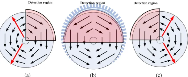
Figure 3.7 A top view of segmenting an omni-image. ... 40 Figure 4.1 Illustration of selecting the detection region where the red points represent the spots on which optical flows need be found. (a) Detection region used

(11)

in the case of turning to the right. (b) Detection region used in the case of moving forward. (c) Detection region used in the case of turning to the left. ... 43 Figure 4.2 The optical flow pattern and the corresponding detection region. (a) The case of turning to the right. (b) The case of moving forward. (c) The case of turning to the left. ... 44 Figure 4.3 An example of results of implementing the optical flow analysis method. (a)

An image frame taken at time t. (b) An image frame taken at time t + dt. (c) The result of the motion vectors produced by the optical flow analysis method with (a) and (b) as inputs. ... 47 Figure 4.4 Transformation of a motion vector from the ICS to the WCS. (a) An illustration of the camera system and the motion vector. (b) The ray tracing of a scene point P on the ground projected on the hyperboloidal-shaped mirror... 49 Figure 4.5 A distribution chart of the direction angle of motion vectors. ... 51 Figure 4.6 A graph of finite state machine proposed to determine the moving direction.

... 52

Figure 4.7 Structure of the communication between two laptops used in this study. .. 54 Figure 4.8 An example of results of optical flow analysis on omni-images and corresponding perspective-view images, where the red arrowheads represent motion vectors. (a) Optical flows of “turning to the left.” (b) Optical flow of “moving forward.” (c) Optical flow of “turning to the right.” (d) ~ (e) Corresponding perspective-view images of (a) ~ (c), respectively. ... 57 Figure 4.9 The car-driving assistance by analyzing omni-images of the surrounding environment. ... 57 Figure 4.10 An interface for inspecting the sequential driving record. ... 59 Figure 4.11 The result of inspecting the driving history. (a) The omni-image and the perspective-view image obtained from transforming the omni-image acquired with the right-front camera. (b) The omni-image and the perspective-view image obtained from transforming the omni-image acquired with the left-rear camera. ... 60 Figure 4.12 A flowchart of sequential driving recording for off-line inspection. ... 61 Figure 5.1 A flow chart of static car detection with a static video surveillance vehicle.

... 63 Figure 5.2 The interface for ground learning. (a) An example of initializing the region of the ground. (b) An example of selecting the ground region by a user. .. 64 Figure 5.3 Related images of noise elimination. (a) The original omni-image. (b) The bi-level image of eliminating the ground and thresholding in the image (a).

(12)

... 67 Figure 5.4 The bi-level images of the nearby static car detection. (a) The image before noise elimination. (b) The image after noise elimination. ... 67 Figure 5.5 An illustration of the region growing process  the blue region represents the car region and the white region represents the non-car region. Once the scan point finds the car region, the region growing process starts. ... 69

Figure 5.6 An illustration of detecting the edge points in bi-level image... 70 Figure 5.7 An example of edge-point extraction. (a) The bi-level image b for searching the bottom-edge points of the vehicle window (a) An image to show the result of finding the edge points, and the red points represent the edge points corresponding to (a). ... 72 Figure 5.8 The result of edge point extraction. (a) The original omni-image acquired with the omni-camera. (b) The image with the bottom-edge points of the vehicle window represented by red points. ... 74 Figure 5.9 An example of simple linear regression, where the blue points represent the edge points transformed into the WCS and the black line is the result. .... 76 Figure 5.10 A surround map from the top view... 78 Figure 6.1 Flowchart of nearby car detection with a moving video surveillance vehicle. ... 80 Figure 6.2 An example of block-based omni-image  the block region is the video surveillance vehicle roof that we ignore and the red points are the selected points. ... 81 Figure 6.3 A result of separating the car region from the non-car region, where the red points are used to represent the car region and the green points to represent the non-car region. ... 83 Figure 6.4 An illustration of k-means algorithm. (a) The image of initialize the cluster centers. (b) The image of associating every data with the nearest mean. (c) The image of reassigning the cluster centers. (d) The result image of k-means algorithm. ... 84 Figure 6.5 A result of region growing by the color information. (a) An image to show the result of the region growing, and the purple points represent the growing region. (b) The corresponding bi-level image of the image (a). ... 89

Figure 6.6 A rectangular-shaped car model and the corresponding mask. (a) A blue region of rectangular-shaped model and its representive points in the WCS. (b) The mask image. ... 90 Figure 6.7 The result of mask in the omni-image. (a) The near mask with respect to the video surveillance vehicle. (b) The far mask with respect to the video surveillance vehicle. ... 92 Figure 6.8 A result of matching a detected car by a mask  the yellow region

(13)

represents the detected car and the blue mask represents the result of the rectangular-shaped model transformation... 94 Figure 6.9 Flowchart of updating the car state. ... 96 Figure 6.10 The result of detecting the static nearby car with a moving video surveillance vehicle. (a) The original omni-image. (b) The surround map from the top view... 97

Figure 7.1 An experimental result of generating the perspective-view image. (a) An original omni-image. (b) The perspective-view image of the right-rear direction. (c) The perspective-view image of the rear direction. (d) The perspective-view image of the left-rear direction. ... 99 Figure 7.2 A real example of car direction detection and display of corresponding perspective-view images. (a) The case of turning to the left. (c) The case of turning to the right. (e) The case of moving forward. (b), (d), and (f) The perspective-view images corresponding to (a), (c), (e), respectively. ... 100 Figure 7.3 The experimental result of monitoring a nearby car around a static video surveillance vehicle. (a) The omni-image acquired with an upper camera. (b) The omni-image acquired with a lower camera. (c) The surround map from the top view. Note that the direction of an object is 180o reversed in the omni-image when compared with the real situation as illustrated in (c). ... 102 Figure 7.4 An illustration of the detecting a nearby static car with a moving video surveillance vehicle. ... 103 Figure 7.5 The result of a nearby static car detection with a moving video surveillance vehicle. (a)~ (f) The results of detecting a nearby car parked at the road side and the generated top-view surround maps. Note that the direction of an object is 180o reversed in the omni-image when compared with the real situation as illustrated in (b) (d) (f). ... 104 Figure 7.6 An illustration of the detecting a nearby moving car with a moving video surveillance vehicle. ... 105 Figure 7.7 The result of a nearby moving car detection with a moving video surveillance vehicle. (a)~ (f) The result of detecting a moving car. Note that the direction of an object is 180o reversed in the omni-image when compared with the real situation as illustrated in (b) (d) (f). ... 105

(14)

LIST OF TABLES

Table 3.1 An example of the pano-mapping table. ……….32 Table 3.2 An example of the r- mapping table. ………33 Table 4.1 The range of the angles of the three vehicle moving directions…………..51

(15)

Chapter 1 Introduction

1.1 Motivation

Nowadays, because the computer technology progresses quickly, video cameras are getting more popular and used more widely. In people’s daily life, video cameras can be used to improve human beings’ welfare. For example, people often equip cars with driving-assistance systems like digital driving recorders or car-backing monitoring systems. With the assistance of cameras in these systems, a driver is able to observe surrounding environments easily. Once a traffic accident occurs, he/she can clarify the responsibility for the event by inspecting the video record.

Moreover, video cameras are also useful for developing vision-based techniques for many applications. Through image processing and other techniques, much information can be obtained from images captured with video cameras. For example, a license plate recognition system or a face recognition system requires the use of video cameras to capture images for analysis of specific objects. In this study, it is desired to design a video surveillance system using video cameras on a vehicle, called video surveillance vehicle, for car-driving assistance and car surrounding monitoring applications.

Most researches of vision-based techniques for the mentioned applications are based on the use of traditional projective cameras; however, the limited field of view (FOV) of the traditional camera is a problem. For instance, only the scene in front of a car can be seen when a projective camera is affixed to the car to “see” forward. If we

(16)

want to monitor the entire car surrounding, four or more cameras are required. The requirement of extra cameras to cover the entire surrounding will raise the cost and complexity to develop a video surveillance system on the car. Therefore, we choose omni-cameras (or simply omni-cameras) to be the imaging devices in this study. Each device consists of two axis-aligned omni-cameras. A wider view of the environment around the video surveillance vehicle can be covered by such a camera system.

Besides, most vision-based systems are affixed to some pre-determined places, such as ceilings or utility poles. It is a difficult task to move a system of such a nature entirely to another place to do surveillance works. In this study, we set up two pairs of omni-cameras on the roof of a video surveillance vehicle. With the camera system being carried, the vehicle can move to any place to conduct surveillance works. Furthermore, the cameras equipped on the video surveillance vehicle can also be used to develop functions for various applications.

To sum up, the goal of this study is to develop a video surveillance system on a video surveillance vehicle for the applications of car-driving assistance and car surrounding monitoring. The system is composed of two pairs of two-camera omni-imaging devices, each consisting of two vertically-aligned omni-cameras, which are affixed to the surveillance’s roof. With the advantages of mobility of the video surveillance vehicle and the wide FOV’s of the omni-cameras, we can develop a mobile surveillance system to monitor car surroundings completely for the two applications. Listed below are the more detailed desired capabilities of the proposed system.

(1) The surrounding environment images are captured by omni-cameras, and the captured image sequence is analyzed to decide the driving direction of the vehicle and generate the perspective-view image of the car surrounding environment with respect to a selected view direction.

(17)

(2) The proposed video surveillance system is able to detect any static surrounding car parked at the nearby roadside, and displays a surround map to show its relative position with respect to the surveillance vehicle from the top view.

(3) When the video surveillance vehicle is moving, the proposed video surveillance system can detect a static car or a passing car in the nearby surrounding as well, and displays a top-view surround map as mentioned above to show the relative position of the car.

1.2 Survey of Related Studies

In this section, we conduct a survey of related studies about video surveillance, including designs of omni-cameras for uses on vehicles, techniques for surrounding vehicle detection, and the optical flow method which we use in the proposed video surveillance system for various purposes.

In recent years, video surveillance for various applications has been widely investigated. Christian et al. [1] proposed a method to track concerned objects based on the use of a video surveillance system on a vehicle. The vision-based surveillance system can be used to monitor a parking lot or conduct traffic surveillance works [2, 3].

An omni-camera in a video surveillance system is useful for localizing objects. It includes just a projective camera and a mirror. Onoe et al. [4] and Mituyosi et al. [5] proposed methods to track people on video surveillance systems with omni-cameras. Moreover, applications using different combinations of projective cameras and mirrors to construct new types of omni-imaging systems have also been investigated. For example, a method to obtain stereo information for mobile robot navigation with an omni-imaging system which consists of two mirrors and one camera was proposed

(18)

by He et al. [6]. Also, Koyasu et al. [7] proposed a stereo system which consists of two omni-cameras aligned vertically for obstacle detection and tracking.

In this study, to obtain the stereo information from omni-images, we adopt the space-mapping method proposed by Jeng and Tsai [8] to calibrate omni-cameras without knowing the intrinsic and extrinsic parameters of the cameras. Moreover, because omni-images captured with omni-cameras may be processed to produce panoramic images and estimate the relevant stereo information of surrounding objects, many studies replace conventional projective cameras with omni-cameras. For example, to assist a driver to observe the entire car surrounding environment, researchers proposed techniques to generate surrounding bird’s-eye views from omni-images, such as Ehlgen and Pajdla [9]. Gandhi and Trivedi [10] also proposed a method to use omni-cameras to conduct detection of moving persons and vehicles on a mobile platform. By the way, the large FOV’s of an omni-camera is a great benefit to monitor the entire surrounding environment. Some researchers combine this advantage and the mobility of vehicles to develop applications [11-13].

In addition, the optical flow method is useful for analyzing the motions within two consecutive image frames. Lucas and Kanade [14] proposed a method to compute the displacement of the image contents between two image frames within the neighborhood of a point. In many studies, the optical flow method is used to detect ego-motions for analyzing the car moving direction. Kim and Suga [15] proposed a method to detect a moving obstacle using an optical flow method for a mobile robot with an omni-camera.

For long, the topic of vehicle detection has been widely studied. Various techniques were proposed to detect vehicles. For instance, background subtraction is a common technique used to extract vehicles [16, 17]. Tsai et al. [18] proposed a method to conduct vehicle detection from static images using color and edges

(19)

information. In this study, we propose methods to detect a static surrounding car by ground-region subtraction and to detect a moving car by using the motion vectors and color information of the car.

1.3 Overview of Proposed Methods

1.3.1 Terminologies

The definitions of some related terms used in this study are described as follows. 1. Omni-camera: a camera system with a traditional projective camera and a

reflective mirror which can be used to capture images of 360-degree FOV’s. 2. Omni-image: an image captured with an omni-camera.

3. Video surveillance vehicle: a car with a pair of two-camera omni-imaging devices equipped on the car roof as well as two laptops for use as control units inside the car to develop a video surveillance system.

4. Optical flow: a method to estimate the motions of shapes, surfaces, and edges of concerned objects between two sequential images.

5. Motion Vector: motion vectors produced by the optical flow method to represent the velocity and direction of a concerned object.

6. Perspective-view image: an image obtained by projecting a scene onto a flat surface as it is seen by the human eye.

7. Surround map: an image showing the relative position of a surrounding car from the top view.

(20)

1.3.2 Brief Descriptions of Proposed System

There are four goals in developing the proposed system as described in the following.

1. The system is able to analyze the car driving direction using the consecutively acquired omni-images and display corresponding perspective-view images to the driver.

2. The system is capable of recording the surrounding images during driving and let the user see the perspective-view image in any selected view direction constructed from these sequential images as well as inspect the sequential images off-line.

3. The system is able to monitor a static surrounding car and obtain related stereo information of it to generate and display a top-view surround map.

4. The proposed system is able to monitor a passing car or a static car in the surrounding environment when the surveillance vehicle is moving, and display a top-view surround map to show its relative position.

In order to achieve the above goals, the following are the major steps of the system process of the proposed video surveillance system.

1. Set up the previously-mentioned pair of two-camera omni-image devices on the roof of the video surveillance vehicle with one on the front-right corner and the other on the rear-left corner of the car roof.

2. Calibrate the omni-cameras for six outward view directions and use the space-mapping method to generate six corresponding pano-mapping tables. 3. While the surveillance vehicle is moving, analyze its moving direction by the

(21)

coordinate system (WCS), and estimate the moving directions by some pattern recognition methods.

4. Generate a perspective-view image according to the driver’s selection of the view direction by projecting an omni-image onto a flat surface by looking up the pano-mapping tables.

5. Detect any static surrounding car by elimination of the ground regions in an omni-image, extract the edge points of a detected car, use the points to compute the stereo information of the detected car, and display the corresponding top-view surround map including the car.

6. Detect a passing-by car or a static surrounding car by the optical flow method, use the lengths of these motion vectors to roughly separate ground regions and car regions, apply region growing based on the color information to find the complete car shape, estimate the stereo information of the car, and generate a top-view surround map to show the relative position of the car.

1.4 Contributions

The following is a list of the major contributions made in this study.

1. A method for obtaining the stereo information of a concerned object by the pano-mapping method using a pair of two-camera omni-imaging devices is proposed.

2. A method for constructing the pano-mapping tables for six outward view directions is proposed.

3. A method for constructing tables of perspective mapping described in detail in Chapter 3 between the omni-images and the perspective-view image to shorten the processing time of image transformation is proposed.

(22)

4. A method for analyzing the driving directions of the video surveillance vehicle by the optical flow method and using the direction to generate corresponding perspective-view images is proposed.

5. A local network is constructed, which integrates a pair of two-camera omni-directional imaging devices and two laptop computers for video surveillance use.

6. A method for detecting a static surrounding car and computing its accurate 3D information is proposed.

7. A method to detect a moving surrounding car or a static surrounding car by thresholding the lengths of motion vectors and extracting the region of the car is proposed.

8. A method for generating rectangular-shaped models and transforming them into the camera coordinate system to mask a detected car for computing the location of the car is proposed.

9. A method for generating a surround map to display the relative location of a detected car in an acquired omni-image with respect to the surveillance vehicle is proposed.

1.5 Thesis Organization

In the remainder of this thesis, we introduce the system configuration and the idea of the proposed method in Chapter 2. The designs of the camera system and the method to obtain stereo information are also described. In Chapter 3, the construction of the pano-mapping tables by the space-mapping technique and the technique of using the pano-mapping tables for unwarping an omni-image into multiple perspective-view images are described. In Chapter 4, the proposed methods for

(23)

computing the car moving direction and for generating the corresponding perspective-view image are described. In Chapter 5, the proposed method for detecting a static surrounding car is described. In Chapter 6, the proposed method for detecting a moving surrounding car is described. In Chapter 7, experimental results and discussions are included. Finally, conclusions and some suggestions for future works are given in Chapter 8.

(24)

Chapter 2 Idea of Proposed Methods and

System Design

2.1 Idea of Analyzing Surrounding

Environment and Vehicles

In order to monitor the surrounding environment of the video surveillance vehicle, we choose omni-cameras instead of traditional projective cameras to acquire environment images. The acquired omni-images can be used to generate corresponding panoramic images and so provide necessary information for security monitoring or driving assistance. In this study we affix a pair of two-camera omni-imaging devices to the surveillance vehicle roof for this purpose as shown in Figure 2.1. Each device includes two omni-cameras aligned coaxially and back to back, as mentioned previously.

(a) (b)

Figure 2.1 The video surveillance vehicle used in this study with a pair of two-camera omni-directional devices affixed on the car roof. (a) A front view of the video surveillance vehicle. (b) A side view of the video surveillance vehicle.

(25)

An advantage of the mobility of the video surveillance vehicle is that we can move the entire system to everywhere to conduct surveillance works. Besides, to get useful views as far as possible, we decided to affix one omni-image device at the right-front position of the surveillance vehicle roof, and the other at the left-rear. As illustrated in Figure 2.2, if instead we affixed a device at the front (or back) middle of the vehicle roof, a half of the acquired omni-image is useless, covering just the roof of the vehicle.

(a) (b)

Figure 2.1 Positions of cameras affixed to the video surveillance vehicle roof and the corresponding FOV. (a) The omni-camera is affixed at the rear-middle of the car roof. (b) The omni-camera is affixed at the right-rear of the car roof.

Many car accidents occur because the driver ignores “blind spots” which cannot be seen in the mirrors equipped inside and outside the car. To show the views of these blind spots, we can use the mentioned pair of omni-imaging devices on the surveillance vehicle roof to generate perspective-view images around the car on every driver-specified view direction. The construction of the perspective-view image from an omni-image conducted in this study is based on the space-mapping method proposed by Jeng and Tsai [8].

In addition, when a driver wants to turn to the left or to the right, the blind spots behind the surveillance vehicle are apt to be neglected. Therefore, we analyze the

(26)

motion vectors produced by the optical flow method in consecutively acquired images. With these motions, we can estimate the vehicle moving direction and show the corresponding perspective-view image. During driving, we can also store images captured with omni-cameras. As a driver recorder, the system can then display these images in sequence, or let the user to choose a view direction and display the corresponding perspective-view image for closer observation.

Furthermore, in order to detect a static car parked at the nearby roadside and compute the stereo information of it, we use the color feature to separate the car region from the ground in the acquired omni-image. In doing this, we assume that the background is uncomplicated with almost the same color as that of an asphalt road, and that the color of the detected car is different from the ground presumably. Therefore, the car shape can be extracted as the foreground by elimination of the ground color.

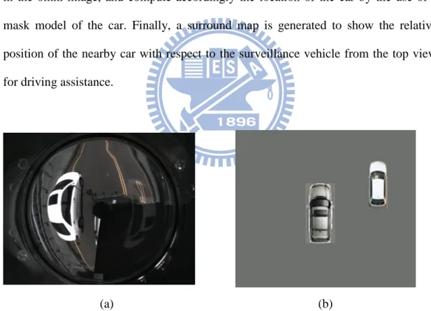
Moreover, we also want to obtain the stereo information of the detected car. For this, the corresponding points of the bottom-window edge of the car in a pair of images captured with the upper omni-camera and the lower omni-camera are chosen. Then, the image data of these points are used to compute the desired stereo information. However, some points like the outlier ones might incur errors in the computed stereo information, so they are eliminated by a linear regression method in this study. As a result, we can compute the location of the car by using the image data of the remaining points, and generate accordingly a surround map. An example of the result of this process is shown in Fig. 2.3.

Finally, we use motion vectors to analyze the acquired omni-images for several purposes. Such motion vectors are produced from consecutive omni-images directly when concerned objects are moving in the omni-images. Specifically, the angles and the lengths of these motion vectors are almost all equal when the vehicle is driven on

(27)

a flat field with roughly identical texture everywhere. Accordingly, if another car is driven aside to overtake the surveillance vehicle gradually, the angles of the motion vectors of the car will differ from those of the motion vectors produced from the entire environment. This characteristic so can be utilized to detect a nearby car in an acquired omni-image.

Another feature used in this study is motion vector length. If a concerned object is higher than the ground, the lengths of the motion vectors yielded by it will be longer than those yielded by the ground. After roughly locating the car using this feature, we use a third feature, the color of the monitored car, to grow the car region in the omni-image, and compute accordingly the location of the car by the use of a mask model of the car. Finally, a surround map is generated to show the relative position of the nearby car with respect to the surveillance vehicle from the top view for driving assistance.

(a) (b)

Figure 2.3 An example of static nearby car detection. (a) An omni-image of a static car parked at the nearby roadside. (b) A generated surround map showing the relative position from the top view. Note that the direction of an object is 180o reversed in the omni-image when compared with the real situation as illustrated in (b).

(28)

2.2 System Configuration

In this section, we will describe the video surveillance system elaborately. The proposed system is mainly divided into three parts. The first part is the hardware which includes a video surveillance vehicle, a pair of two-camera omni-directional imaging devices, and two laptop computers. The second part is the software. In this part, we will introduce the software development environment and the accompanying SDK and driver programs for the CCD cameras. The third part is the network. Because we use two laptops to handle the pair of two-camera omni-directional imaging devices, respectively, a local network is used for communication between the two laptops.

2.2.1 Hardware configuration

The surveillance vehicle, named Delica, is made by Mitsubishi Co. It is a 469cm ×169cm×196cm vehicle with a working table and a power supply. System operators may sit inside the surveillance vehicle to operate the laptop computers and monitor the entire surrounding environment. Moreover, a steel frame is affixed to the car roof, on which the omni-image devices can be affixed. And four extension USB cords crossing the video surveillance vehicle were added to receive images which are captured with the two omni-imaging devices. Detailed descriptions of the imaging devices will be given in Section 2.3. The entire video surveillance system is shown in Fig. 2.4.

In order to control the entire video surveillance system, in this study we use two laptops as control units, each handling an omni-imaging device. Both laptops are produced by TOSHIBA Computer Inc., and their detailed specifications are listed in

(29)

Table 2.1. To exchange commands and images between the two laptops, we use a cross-over cable to connect then and set up a local network for between-computer communication. Local Network Computer A Computer B Cross-over cable Video surveillance car Camera System A Camera System B Affixed on Affixed on

Figure2.4 Structure of the proposed surveillance system.

Table 2.1 Specifications of the laptop computers used in this study.

Tecra M11 Satellite A660

CPU Intel Core i7-620M

2.66/3.33GHz

Intel Core i5-480M 2.66/2.93GHz

RAM 4G DDR3 1066MHz 2G DDR3 1066MHz

GPU nVidia NVS 2100M ATI HD5650

(30)

2.2.2 Software configuration

We use Borland C++ Builder (BCB) V6 as a developed platform to build our video surveillance system. The BCB is a program development tool for the operating system of Windows; therefore, we can create a graphic user interface (GUI) conveniently and quickly. The programming language we use is C++. It is a widely used language. One of the laptops, the Tecra M11 computer, uses the operating system of Windows 7, and the other, Satellite A660, uses Windows XP.

Before developing a video surveillance system, we have to install the drivers of the ARTCAM-200SO cameras and those of the ARTCAM-200SS cameras in the laptop computers. The camera company also provides corresponding software development kits (SDKs) and some simple source codes. Accordingly, we can adjust the parameters of each camera, such as the value of exposure or the global color gain, through the SDK. The SDK is an object-oriented toolkit, and the camera company not only provides the BCB version but also the C, VB.NET, C#.NET or Delphi version to the programmers.

2.2.3 Network Configuration

COMA COMB

Local Network

Control signals Control signals & Omni-image & Perspective-view image of COMA

USB Port USB Port Camera System A Camera System B

(31)

A network configuration is needed for communication between two laptop computers because four omni-images are acquired from the pair of two-camera omni-directional imaging devices and each imaging device is processed by a respective laptop. As a result, to communicate between the two laptops, we set up a local area network to send images and control signals.

As shown in Fig. 2.5, laptop computer COMB is used to display the

perspective-view image and the acquired omni-image, therefore, laptop computer COMB needs to receive these images from COMA through the local network.

Moreover, the control signals of the selected view direction produced by COMA are

sent to COMB for generating the corresponding perspective-view image.

2.3 Review of Adopted Camera System

and 3D Data Acquisition Process

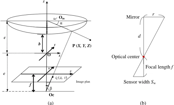
In this section, we review the adopted camera system and the corresponding 3D data acquisition process proposed in Yuan el at. [19]. First of all, we introduce the detail of building the camera system. The entire system includes four lenses of model LV0612H, two CMOS cameras of model ARTCAM-200SO, and two CMOS cameras of model ARTCAM-200MI. Table 2.2 lists the specifications of the COMS cameras.

To build an omni-camera, the most important task is to combine a projective CCD camera and a hyperboloidal-shaped mirror into an omni-camera. In the design process of the omni-camera, an optics manufacturer was requested to produce hyperboloidal-shaped mirrors. The parameters of each of the mirrors are described here. The radius r of the hyperboloidal-shaped mirror is 4cm. The projective camera has a focal length f of 6 mm and a sensor width Sw of 2.4mm. And the axis of the

(32)

camera is aligned with the axis of the hyperboloidal-shaped mirror. Therefore, by the principle of similar triangles, the distance d between the optical center of the lens and the mirror center can be computed from the following equation:

w

d f

r  S . (2.1)

Also, as shown in Fig. 2.6(a), the hyperboloidal shape of the mirror in the camera coordinate system may be described as:

2 2 2 2 2 2 1, R Z R X Y a b     . (2.2)

To get the parameters a and b of the hyperboloidal shape of the mirror, first the elevation angle α in Figure 2.6 (a) can be obtained from the relation between the CCS and the ICS of an omni-camera system derived by Wu and Tsai [20] as follows.

2 2 2 2 ( ) sin 2 tan . ( ) cos b c bc b c        (2.3)

Furthermore, by the simple formula d = 2c where the value c is the distance from the center O shown in Fig. 2.6 to the mirror center Om, the angles θ and β can be

computed as follows: 1 tan , 2 . 2 r c         (2.4)

In Eq. (2.3), let the omni-camera have the largest FOV, the incidence angle α be set 0, and by using Eq. (2.4), the parameter b can be obtained by solving Eq. (2.3).Finally, the parameter a is derived from the following equation:

2 2

(33)

f b Image plan Oc O β α c c Z X Y U V Om P (X, Y, Z) q(u, v) r d Focal length f Sensor width Sw Mirror Optical center (a) (b)

Figure 2.6 (a) Relation between the world coordinates and the image coordinates (b) Geometry between the mirror and the CMOS sensor in camera.

Each omni-camera was built with these parameter values, and a two-camera omni-directional device can be constructed with two omni-cameras aligned vertically.

Table 2.2 Specifications of used COMS cameras.

ARTCAM-200SO ARTCAM-200MI

Resolution 2.0 M pixels(1600*1200) 2.0 M pixels(1600*1200) Dimension 33mm × 33mm × 50mm 33mm × 33mm × 50mm CMOS sensor size 1/2” (6.4×4.8mm) 1/2” (6.4×4.8mm)

Mount C-mount C-mount

Frame per second 8 fps 5 fps

Direct show camera Yes No

After describing the way of building the cameras, we now describe the adopted method to compute stereo information from a two-camera omni-directional imaging device. In the omni-imaging device, relevant 3D data can be computed by two elevation angles and an azimuth angle of a scene point P. As shown in Figure 2.7(a), the point P projects on each hyperboloidal-shaped mirror and forms a pair of

(34)

corresponding points in the upper image and the lower image captured with a two-camera omni-imaging device. The elevation angles of point P on the hyperboloidal-shaped mirrors are defined as α1 and α2, respectively. Also, the center of the upper hyperboloidal-shaped mirror is assumed to be the origin of the world coordinates (0, 0, 0). It is desired now to compute the stereo depth data of point P in terms of the two elevation angles α1 and α2.

(a) (b)

Figure2.7 Computation of depth using the two-camera omni-directional imaging device. (a) The ray tracing of a scene point P in the imaging device with a hyperboloidal-shaped mirror. (b) A triangle in detail (part of (a)).

To obtain stereo depth of a scene point P(x, y, z), finding two elevation angles α1 and α2 by looking up a pano-mapping table is required, and the construction of pano-mapping table will be described in Chapter 3. As shown in Figure 2.7(b), the distance d between the point P and the upper mirror center c1 is computed by the triangulation principle shown in Figure 2.7(a) using the equation below:

2 1 2

sin(90 ) sin( )

d b

   

  , (2.6)

(35)

(2.6) may be reduced to be the following equation by trigonometry:

2

1 2 1 2

1 1 2

cos ,

sin cos cos sin

1

.

cos tan tan

b d b d                 (2.7)

As a result, the horizontal distance dw and the vertical distance Z may be computed as follows: 1 1 1 2 1 1 2 tan sin , tan tan 1 cos . tan tan z d b dw d b                (2.8)

Assume that point P at world coordinates (x, y, z) is projected on a point I at image coordinates (u, v) in the image coordinate system (ICS). Then, we can use point I to calculate the azimuth angle . A triangulation which is illustrated in Figure 2.8 includes an azimuth angle  between the X-axis and point I. As a result, the azimuth angle  can be computed by the following equation:

1 1 2 2 2 2 cos sin v u v u v   _  _    . (2.9)

According to the characteristic that the axis of the camera is aligned vertically with the axis of the hyperboloidal-shaped mirror as well as the rotation-invariance property of omni-imaging, the azimuth angle of a point in the ICS is the same as that of the corresponding point in the WCS. We can calculate the parameters x and y by the distance dw and the azimuth angle  in the WCS as follows:

1 2 1 2 1 cos cos , tan tan 1 sin sin . tan tan x dw b y dw b                     (2.10)

(36)

can be transformed to an elevation angle and an azimuth angle. Once the azimuth angle  and a pair of elevation angles α1 and α2 are obtained, we are able to compute the location of point P in the WCS. Therefore, a pair of matching points (one is in an omni-image taken by the upper omni-camera, and the other is in an omni-image taken by the lower omni-camera) is known, the stereo information of the unique point in the WCS may be obtained. θ θ dw f I(u,v) U V P(x,y,z) X Z Y Upper hyperboloidal-shaped mirror center

c1 (0, 0, 0)

Figure2.8 System configuration of upper omni-camera with a hyperboloidal-shaped mirror.

2.4 System Processes

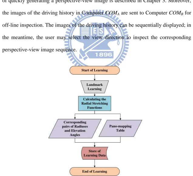
To get stereo information from a pair of two-camera omni-imaging devices, the omni-cameras need to be calibrated. For this purpose, the space-mapping technique is applied, and the technique is based on the use of a pano-mapping table. The process of constructing the table is shown by Fig. 2.9. We will introduce the process in Chapter 3 elaborately. Moreover, the method to unwarp an omni-image into a perspective-view image using the pano-mapping table is also described in Chapter 3.

(37)

The above-mentioned process is an advance preparation before developing the system. As shown in Figure 2.10, to develop the car-driving assistance application, we need to read the related tables at the beginning. Computer COMA used in this study is

responsible for analyzing omni-images of the surrounding environment by the optical flow method and estimating the moving direction of the video surveillance vehicle by the produced motion vectors. Then, the analyzed result and acquired images are sent to another computer COMB for generating the corresponding perspective-view image.

The process will be introduced elaborately in Chapter 4. Computer COMB generates

the corresponding perspective-view images with respect to these signals. The method of quickly generating a perspective-view image is described in Chapter 3. Moreover, the images of the driving history in Computer COMA are sent to Computer COMB for

off-line inspection. The images of the driving history can be sequentially displayed; in the meantime, the user may select the view direction to inspect the corresponding perspective-view image sequence.

Start of Learning Landmark Learning Calculating the Radial Stretching Functions Corresponding pairs of Radiuses and Elevation Angles Pano-mapping Table Store of Learning Data End of Learning

(38)

Start of Video Surveillance

Pano-mapping

Table mapping tablePerspective

Sequential omni-images Load Tables Computing motion vectors Analysis of the Moving

Directions

Start of Video Surveillance

Pano-mapping

Table Sequential omni-images Load Tables

Send Command and images to Another Computer

Constructing Correspondence Perspective-view Image Control Signal &

Omni-images Display Perspective-view Image Store images Store images Computer A with Camera System A Computer B with Camera System B Mouse Motion Image Buffer

Figure 2.10 Flowchart of the moving direction analysis.

Both the application of nearby static car detection with a static video surveillance vehicle and the application of nearby static or moving car detection with a moving video surveillance vehicle require reading table files as a preparation task as shown in Fig. 2.11. In the application of nearby static car detection with a static video surveillance vehicle, two omni-images are captured with a two-camera omni-directional imaging device and the detection process is conducted. Finally, the stereo information of the car is computed. The detailed process will be introduced in Chapter 5. Additionally, nearby static or moving car detection with a moving video surveillance vehicle requires two consecutively acquired images to conduct the detection process. We need to create an image buffer to keep the previous image and acquire a current image with the omni-camera for analyzing the omni-images of the surrounding environment. The detection and position estimation of the static or moving car will be described in Chapter 6. Finally, the two applications will both

(39)

display the surround map. Both tasks are required complex processes, so we will introduce above-mentioned processes in the remaining chapters elaborately

Start of Video Surveillance

Sequential omni-images Pano-mapping Tables Detection of a static surrounding car Estimating 3D Data of the car Load Tables Display Surround Map Detection of a moving surrounding car Estimating 3D Data of the car Image buffer

(40)

Chapter 3 Generation of Perspective-view

Images Using Pano-mapping Tables

In this chapter, we describe the details of the scheme we use to generate perspective-view images from omni-images acquired with the omni-image devices attached to the roof of the video surveillance vehicle used in this study. Before describing the detail in Sections 3.2 through 3.4, we review first in Section 3.1 a space-mapping technique [8] we adopt for use in coordinate mapping from the omni-image to the perspective-view image.

3.1 Review of Adopted Pano-mapping

Method for Omni-image

Unwarping

The scene appearing in an omni-image is distorted due to the light reflection on the hyperboloidal-shaped mirror. In order to facilitate observation of the distorted image, we want to unwarp the omni-image into a perspective-view image. The conventional method for unwarping the omni-image requires the parameters of the hyperboloidal-shaped mirror and the camera. However, sometimes we cannot obtain such parameter information completely. The space-mapping technique proposed by Jeng and Tsai [8] can solve this problem and is adopted in this study. The technique is based on the use of a so-called pano-mapping table which records the relationship

(41)

between the pixel in the image and the elevation and azimuth angles of the corresponding world-space point with respect to the focal center of the mirror. The creation of the pano-mapping table includes three major steps: (1) landmark learning; (2) estimation of coefficients of radial stretching function; and (3) filling of the pano-mapping table entries. We will introduce these steps in Section 3.2.

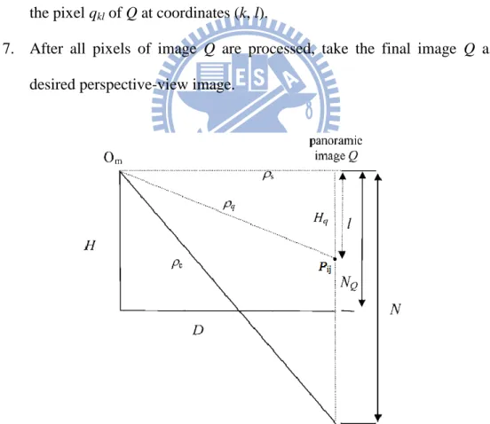
With the use of the pano-mapping table, an omni-image can be transformed into perspective-view images. The transformation process will be introduced in Section 3.3. Besides, the process of generating perspective-view images is generally complicated. To shorten the computation time, we divide the omni-image into portions seen from six outward viewing directions, and create a table to record the relationship between each of the six omni-image portions and its perspective-view image.

3.2 Construction of Pano-mapping

Table

3.2.1 Landmark Learning

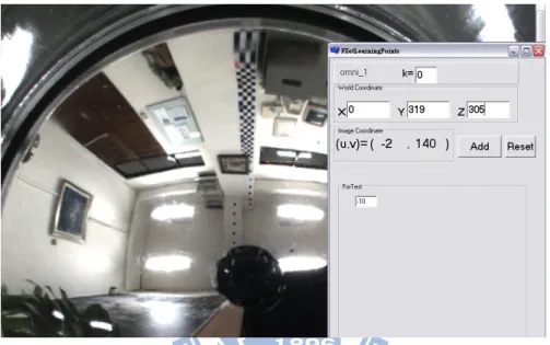
The first step of creating the pano-mapping table is to establish several pairs of world-space point and the corresponding image point in the taken omni-image. The coordinates of the world-space points in these pairs, called landmark points, are measured manually with respect to a selected origin in the world space. To facilitate selecting the landmark point pairs, a user interface was provided, as shown in Fig. 3.1. We define the focal center Oc in the image coordinates (u0, v0) as the origin in the image coordinates system and Om as the focal point of the hyperboloidal-shaped mirror at the world coordinates (X0, Y0, Z0). Assume that n sets of corresponding

(42)

points are selected, and each set include a landmark point pi at image coordinate (ui, vi)

with respect to Oc as well as the corresponding world-space point Pi at the coordinates (Xi, Yi, Zi) with respect to the origin Om, where i = 0, 1, …, n  1. In this step, the construction of a mapping table requires learning at least six landmark points. And the more landmark points are selected, the more accurate the table is.

Figure 3.1 An interface to for user to select the landmark points.

3.2.2 Estimation of Coefficients of Radial Stretching

Function

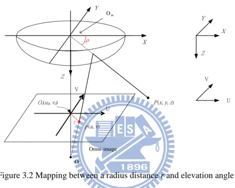
Due to the nonlinear shape of the hyperboloidal-shaped mirror, the radial-directional mapping must be represented as a non-linear function. As shown in Figure 3.2, each elevation angle corresponds to a radial distance. More specifically, each elevation angle  of a scene spot P at world coordinates (X, Y, Z) corresponds to the radius r of the corresponding point p in the omni-image. Therefore, we want to find out the relationship between the radius r and the elevation angle  by the use of a non-linear function fr, called radial stretching function. In this study, fr is

(43)

approximated by the following 5th-degree polynomial equation: 1 2 3 4 5 0 1 2 3 4 5 ( ) r r f  a  a   a   a   a   a  . (3.1) To compute the desired coefficients a0 through a5, the following algorithm is performed. Om Omni-image Ol X Y P(x, y, z) U V p(u, v) Z X Y Z U V  r Oc(u0, v0)

Figure 3.2 Mapping between a radius distance r and elevation angle ρ.

Algorithm 3.1 Computing the coefficients of the radial stretching function for the mirror.

Input: a set of n landmark point pairs (pk, Pk) selected in advance for the radial

stretching functions fr, where pk is a point in an omni-image I and Pk is the

corresponding point in the world space.

Output: the six coefficients ao through a5 of fr.

Steps.

Step 1. For each selected landmark point pairs, (Pk, pk), including world-space point

Pk at coordinates (Xk, Yk, Zk) in the WCS and image point pk at coordinates

(44)

in the WCS by the following equations: 2 2 1 2 2 ; tan k . k k k k k k Z r u v X Y       (3.2)

Step 2. Substitute rk and k into the equation for estimating fr described by Eq. (3.1)

to obtain n simultaneous equations as follows:

1 2 3 4 5 0 0 0 1 0 2 0 3 0 4 0 5 0 1 2 3 4 5 1 1 0 1 1 2 1 3 1 4 1 5 1 1 2 3 4 5 1 1 0 1 1 2 1 3 1 4 1 5 1 ( ) ( ) ( ) . ri ri n ri n n n n n n r f a a a a a a r f a a a a a a r f a a a a a a                                                              (3.3)

Step 3. Solve the equations in (3.3) to obtain the desired coefficients (a0, a1, a2, a3, a4, a5) for fr by a numerical analysis method.

In the above process of computing the radial stretching function, it is assumed that the mirror is perfect with rotational symmetry in the entire angle range of 0o through 360o. However, this is not the case in real applications; the surface of the hyperboloidal-shaped mirror cannot be so perfect. To increase the accuracy of the estimated fr and so the precision of the constructed pano-mapping table, we divided

the 360o range of azimuth angles of the mirror equally into six parts, each with 60o, and then applied the above process to obtain six radial stretching functions fr1 through

fr6 for the six parts with each fri described by the coefficients a0i through a5i with i = 1, 2, …, 6.

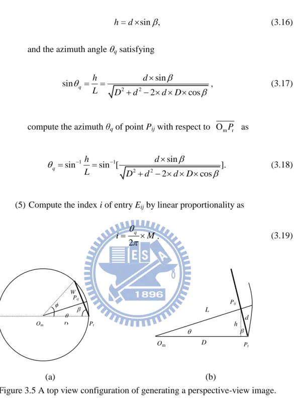
3.2.3 Filling of Pano-mapping Table Entries

The procedure of constructing the pano-mapping table with the radial stretching function for each of the six azimuth angle ranges is described here. The so-called pano-mapping table is a 2-dimensional table with its horizontal and vertical axes

(45)

specifying the azimuth angle  and the elevation angle , respectively. An illustration of the mapping between the azimuth and elevation angle pair of the omni-image and the horizontal and vertical axes of the pano-mapping table, respectively, is shown in Fig. 3.3, and an example of the pano-mapping table is shown in Table 3.1.

Each entry Eij with indices (i, j) in the pano-mapping table corresponds to an

azimuth-elevation angle pair (i,j). The azimuth-elevation pair represents an infinite

set of points on a light ray with the azimuth angle i and the elevation angle j with

respect to the focal center Om in the WCS. We divide the range 2π of the azimuth angles into M intervals and the range of the elevation angles between two pre-selected limits, s and e,into N intervals. Due to the property of rotational invariance of

omni-imaging, the azimuth angle of the scene point P in the WCS with respect to the X-axis is identical to the azimuth angle θ of the corresponding point p in the image with respect to the u-axis. Thai is, we have = .

(a) (b)

Figure 3.3 Illustration of mapping between the azimuth-elevation angle pair of the omni-image and the horizontal and vertical axes of the pano-mapping table, respectively.

With the above estimated six sets of coefficients for the six radial stretching functions, the corresponding pano-mapping table Tpm can be filled with the corresponding image coordinates by the following algorithm.

(46)

Table 3.1 An example of the pano-mapping table. 1 2 3 4 … M 1 (u11, v11) (u21, v21) (u31, v31) (u41, v41) … (uM1, vM1) 2 (u12, v12) (u22, v22) (u32, v32) (u42, v42) … (uM2, vM2)  3 (u13, v13) (u23, v23) (u33, v33) (u43, v43) … (uM3, vM3)  4 (u14, v14) (u24, v24) (u34, v34) (u44, v44) … (uM4, vM4)  … … … …  N (u1N, v1N) (u2N, v2N) (u3N, v3N) (u4N, v4N) … (uMN, vMN)

Algorithm 3.2 Construction of the pano-mapping table.

Input: six coefficient sets of six radial stretching functions fr1 through fr6 for the six

parts of the azimuth angle range mentioned previously.

Output: a pano-mapping table Tpm of the dimension M×N.

Steps.

Step 1. Divide the range 2π of the azimuth angles into M intervals, and compute the ith azimuth angle i by

i = (2i for i = 0, 1, …, M  1. (3.4)

Step 2. Divide a pre-selected range s, e] of the elevation angle into N intervals,

and compute the j-th elevation angle j by

j = [(es)/N]j + s for j = 0, 1, ..., N  1. (3.5)

Step 3. Fill the entry of (i, j) with the corresponding image coordinates (uij, vij)

computedas follows:

cos , sin

i j j i i j j i

u  r  v  r  , (3.6)

where the radius rj is computed by the radial stretching function as follows:

rj = fri(j) = a0i+a1ij1+a2ij2+a3ij3+a4ij4+a5ij5, (3.7)

利用架設在視訊監控車上成對的全方位攝影裝置作週遭環境監控之研究

國 立 交 通 大 學

資訊科學與工程研究所

碩 士 論 文

利用架設在視訊監控車上成對的

全方位攝影裝置作週遭環境監控之研究

A Study on Surrounding Environment Monitoring by a Video

Surveillance Car with Two 2-camera Omni-imaging Devices

研 究 生：陳俊甫

指導教授：蔡文祥 教授

利用架設在視訊監控車上成對的

全方位攝影裝置作週遭環境監控之研究

A Study on Surrounding Environment Monitoring by a Video

Surveillance Car with Two 2-camera Omni-imaging Devices

研 究 生：陳俊甫 Student：Chun-Fu Chen

指導教授：蔡文祥 Advisor：Wen-Hsiang Tsai

國 立 交 通 大 學

多 媒 體 工 程 研 究 所

碩 士 論 文

利用架設在視訊監控車上成對的

全方位攝影裝置作週遭環境監控之研究

研究生: 陳俊甫

指導教授:蔡文祥 博士

國立交通大學資訊科學與工程研究所

摘要

A Study on Surrounding Environment Monitoring

by a Video Surveillance Car with Two 2-camera

Omni-imaging Devices

Student: Chun-Fu Chen

Advisor: Prof. Wen-Hsiang Tsai

Institute of Multimedia Engineering, College of Computer Science

National Chiao Tung University

ABSTRACT

ACKNOWLEDGEMENTS

CONTENTS

LIST OF FIGURES

LIST OF TABLES

Chapter 1

Introduction

1.1 Motivation

1.2 Survey of Related Studies

1.3 Overview of Proposed Methods

1.3.1 Terminologies

1.3.2 Brief Descriptions of Proposed System

1.4 Contributions

1.5 Thesis Organization

Chapter 2

Idea of Proposed Methods and

System Design

2.1 Idea of Analyzing Surrounding

Environment and Vehicles

2.2 System Configuration

2.2.1 Hardware configuration

2.2.2 Software configuration

2.2.3 Network Configuration

2.3 Review of Adopted Camera System

and 3D Data Acquisition Process

2.4 System Processes

Chapter 3

Generation of Perspective-view

Images Using Pano-mapping Tables

3.1 Review of Adopted Pano-mapping

Method for Omni-image

Unwarping

3.2 Construction of Pano-mapping

Table

3.2.1 Landmark Learning

3.2.2 Estimation of Coefficients of Radial Stretching

Function

3.2.3 Filling of Pano-mapping Table Entries

國立交通大學

碩士論文

研究生：陳俊甫

指導教授：蔡文祥教授

研究生：陳俊甫 Student：Chun-Fu Chen

國立交通大學

多媒體工程研究所

碩士論文

指導教授:蔡文祥博士