利用多重解析邊緣梯度的資訊來增強靜態影像畫質

全文

(1)國立交通大學資訊工程系碩士論文. 利用多重解析邊緣梯度的資訊來增強靜態影像畫質. Static Image Enhancement Using Multi-Resolution Gradient Information. 研究生：朱祐吾指導教授：陳. 稔. 教授. 中華民國九十四年七月.

(2) 利用多重解析邊緣梯度的資訊來增強靜態影像畫質 Static Image Enhancement Using Multi-Resolution Gradient Information 研究生：朱祐吾. Student：Yu-wu Chu. 指導教授：陳. Advisor：Zen Chen. 稔國立交通大學資訊工程系碩士論文. A Thesis Submitted to Department of Computer Science and Information Engineering College of Electrical Engineering and Computer Science National Chiao Tung University in partial Fulfillment of the Requirements for the Degree of Master in Computer Science and Information Engineering July 2005 Hsinchu, Taiwan, Republic of China. 中華民國九十四年七月.

(3) 利用多重解析邊緣梯度的資訊來增強靜態影像畫質學生：朱祐吾. 指導教授：陳. 稔博士. 國立交通大學資訊工程學系. 摘要. 本論文的目的在於結合 tone mapping 的技術和以梯度為基礎的陰影去除技術來增強靜態影像畫質，期望結果如同在均勻光源下所獲得的影像一致。因此可以讓辨認系統或是監控系統在不受光影的影響下而能獲得更佳的結果，或是將原本拍攝環境不佳的影像還原成在均勻光源下拍攝的影像。本論文的方法延伸Fattal等人[8]的工作，Fattal等人的方法可以讓太亮或太暗區域的細節部分顯現出來。再搭配我們提出去除模糊陰影邊界的方法，也就是利用模糊邊界辨認器的演算法來偵測陰影的邊界，再調整該區域的梯度，就可以達成去除陰影的目的。在我們的實驗結果中發現這個方法是可行的。不過仍有少數的問題尚待解決，像在陰影處的顏色會有色偏的問題，在模糊邊緣的區域會有一點模糊以及光暈的現象，這些問題如果可以解決，相信辨認系統或是監控系統在未來會有更大突破。. i.

(4) Static Image Enhancement Using Multi-Resolution Gradient Information student：Yu-wu Chu. Advisor：Dr. Zen Chen. Department of Computer Science and Information Engineering National Chiao Tung University. Abstract. The main purpose of this thesis is to combine the technique of tone mapping and gradient based shadow removal technique to enhance the image. We expect to gain the result which is similar to the same scene but with uniform lighting. Therefore, we could let the surveillance or the recognition system gain better result, or restore the image captured under poor condition to a better image as if it was captured under uniform lighting environment. The method of this thesis extends the work of Fattal et al. [8]. Their method could reveal the detail in the bright and dark areas. We simply employ the fuzzy edge classifier to detect the fuzzy edge area, and then adjust the gradient in the fuzzy edge area. In our experimental results, this method is proved feasible. But, there still are some problems remaining to be solved, such as “color shifting” in the shadow area, and blurring the fuzzy edge area and some remaining halo artifact. If these defects can be removed, the surveillance and recognition applications can become much practical.. ii.

(5) Acknowledgement I would like to express my appreciation to my advisor, Dr. Zen Chen, for his helpful guidance, careful supervision and encourage throughout my Master degree. Under his guidance, he lets me know how to analysis and solve the problem. In the past of two years, he has stimulated the research work and also offered an excellent research environment at the PAIS Lab. I would also express my gratitude to all the members in the PAIS Lab, for their encouragements, assistances, useful suggestions and comments. I am grateful to all of my friends for their supports and encouragements. You have made my life wonderful and cheerful. Finally, thank my family for their understanding, supports and loves.. iii.

(6) Contents 摘要 .............................................................................................................................................i Abstract.......................................................................................................................................ii Acknowledgement .....................................................................................................................iii Contents.....................................................................................................................................iv List of tables ...............................................................................................................................v List of Figures............................................................................................................................vi List of Algorithms.....................................................................................................................vii Chapter 1. Introduction ........................................................................................................1 1.1. Motivation ..............................................................................................................1 1.2. Related work...........................................................................................................2 1.3. Contribution............................................................................................................5 1.4. Outline ....................................................................................................................5 Chapter 2. Fundamentals......................................................................................................6 2.1. Estimating the gamma curve of the camera............................................................6 2.2. Reconstructing an image from the gradient field ...................................................8 Chapter 3. Gradient attenuation function ...........................................................................10 3.1. Types of edges ......................................................................................................10 3.2. Distinguishing illuminance from reflectance edges .............................................12 3.3. The illuminance ratios ..........................................................................................14 3.4. Fuzzy or sharp edge..............................................................................................16 Chapter 4. Experimental results .........................................................................................24 4.1. Different parameter setting...................................................................................24 4.1.1. The parameters of the edge classification algorithm ................................24 4.1.2. Adjustment of the gradient in the fuzzy area............................................27 4.1.3. The parameters of the attenuation function ..............................................29 4.2. Comparison with the other methods.....................................................................33 Chapter 5. Conclusion and future work .............................................................................41 5.1. Conclusion ............................................................................................................41 5.2. Future work ..........................................................................................................42 References ................................................................................................................................43. iv.

(7) List of tables TABLE 4.1 THE RESULTS FOR DIFFERENT VALUES OF. τ1 . ........................................................................................ 25. TABLE 4.2 THE RESULTS FOR DIFFERENT VALUES OF. τ2 ......................................................................................... 26. TABLE 4.3 THE EFFECT OF ADJUSTMENT OF THE GRADIENT IN THE FUZZY AREA..................................................... 28 TABLE 4.4 THE RESULTS FOR DIFFERENT VALUES OF α . ........................................................................................ 29 TABLE 4.5 THE RESULTS FOR DIFFERENT VALUES OF. β .......................................................................................... 30. TABLE 4.6 RESULTS BY OUR METHOD. ALTHOUGH THERE ARE SOME PROBLEMS DISCUSSED IN SECTION 4.1, THE SHADOW IS ALMOST GONE............................................................................................................................. 31. v.

(8) List of Figures FIGURE 1.1 THE GRADIENT BASED SHADOW REMOVAL METHOD............................................................................... 2 FIGURE 1.2 RESULTS OBTAINED BY FINLAYSON ET AL.[24] METHOD. THE GRAY TEXTURE ON THE FOOTBALL IS LOST................................................................................................................................................................ 4. FIGURE 1.3 COMPARE THE HW PROPERTY [28]. THE COMPRESSION TECHNIQUE WOULD AFFECT THE RESULT........... 5 FIGURE 1.4 THE FLOW CHART OF OUR SYSTEM ......................................................................................................... 5 FIGURE 3.1 TYPES OF EDGES: ORIENTATION EDGES (O), DEPTH EDGES (D), REFLECTANCE EDGES (R), AND SHADOW EDGES (S). .................................................................................................................................................... 10. FIGURE 3.2 THE CHROMATIC PROPERTY PROPOSED BY RUBIN AND RICHARD [12].................................................. 12 FIGURE 3.3 RESULT BY FATTAL ET AL [8]. THE SHADOW IS STILL THERE. ................................................................ 16 FIGURE 3.4 THE MULTI-RESOLUTION EDGE DETECTION ON THE FUZZY AND THE SHARP EDGE. ............................... 17 FIGURE 3.5 THE MULTI-RESOLUTION EDGE DETECTION OF THE IMAGE IN FIGURE 3.3 (A)....................................... 17 FIGURE 3.6 THE LOCAL STANDARD DEVIATION DIVIDED BY THE LOCAL MEAN. ...................................................... 18 FIGURE 3.7 RESULTS OF THE MULTI-RESOLUTION FUZZY EDGE CLASSIFIER. ........................................................... 20 FIGURE 3.8 FUZZY EDGE PROFILE AND ITS GRADIENT. ............................................................................................ 22 FIGURE 3.9 THE FLOW CHART OF THE ALGORITHM 3.1........................................................................................... 23. (. FIGURE 4.1 THE RESULTS OBTAINED WITH THE SUGGESTED PARAMETERS ( τ1 = 1.0 mean ∇Î j ( x, y ). ),. τ2 = 0.45 ). ................................................................................................................................................ 27 FIGURE 4.2 ORIGINAL IMAGES................................................................................................................................ 35 FIGURE 4.3 RESULTS BY HISTOGRAM EQUALIZATION. ........................................................................................... 36 FIGURE 4.4 RESULTS BY UNILATERAL FILTER. ....................................................................................................... 37 FIGURE 4.5 RESULTS BY BILATERAL FILTER. .......................................................................................................... 38 FIGURE 4.6 RESULTS BY FATTAL’S METHOD............................................................................................................ 39 FIGURE 4.7 RESULTS BY OUR METHOD................................................................................................................... 40. vi.

(9) List of Algorithms ALGORITHM 3.1 FUZZY EDGE CLASSIFIER ALGORITHM........................................................................................... 19 ALGORITHM 3.2 GRADIENT ADJUSTMENT ALGORITHM ........................................................................................... 21. vii.

(10) Chapter 1. Introduction 1.1. Motivation In the nature, a real scene has a high dynamic range of intensity, while the current monitor can only display the low dynamic range image. Human eyes can percept high dynamic range image (HDRI). Recently, HDR image can be reconstructed from a set of photographs of the scene captured under different exposure times [2][3][4]. Several researchers develop novel hardwares to capture the HDR image [5][6]. Thus we can preserve all detail in the scene without loss of information in the areas that are over- or under-exposured. Since the technique of the display device is low dynamic display system. Therefore, we need an additional technique, called tone mapping, to compress HDR image into LDR image without losing the fine detail. In this thesis, our method applies HDR image and tone mapping techniques to preserve the fine detail of the image. The objective is to make the contrast in the dark area and the bright area as same as possible. We extent Fattal et al. [8] work to achieve our goal. Take Figure 1.1 for an example. First, we capture an image containing shadow, and compute the gradient of the image. Then, we mask the area of the shadow edge and set the shadow gradient to zero. After reconstructing the image from the new gradient map, we find that the shadow part in the image is gone. Based on these ideas, we want to design an algorithm to remove the shadow effect in the image.. 1.

(11) (a) The original image. (b) The gradient magnitude of the left image. (c) The new gradient magnitude with set the area of the. (d). shadow edges to zero. The reconstructed from the new gradient magnitude. Figure 1.1 The gradient based shadow removal method.. 1.2. Related work Tone mapping methods can be classified into two main groups [21]: tone reproduction curves (TRCs) and tone reproduction operators (TROs). The main pros of TRCs are simplicity, computational efficiency, and preserved relative contrasts. However, the main cons of them are loss of local contrasts in images. The typical TRC approaches are gamma correction, histogram equalization, and so on. On the contrast, TROs are easy in preserving local contrasts in images, but more complex on computation. The TRO methods can be classified into three groups: human vision system (HVS) base, filter based, and gradient base. HVS based researchers use the computational 2.

(12) model proposed by the work of the psychologists such as [20]. Filter based researchers want to separate original images into reflectance (also called detail or intrinsic image) and illuminance (also called base) images. The basic idea is that the image f(x,y) is regarded as a product, f ( x, y ) = I(x, y)R ( x, y ). (1.1). where R(x, y) is the reflectance and I(x, y) is the illuminance at each point (x, y). If the reflectance and illuminance image can be separated perfectly from the original image, then the HDR image can be compressed by scaling down the illuminance image to get a new illuminance image %I ( x, y ) and re-multiplying the reflectance image. While taking logarithm on the both sides in equation(1.1), we have ln f ( x, y ) = ln I ( x, y ) + ln R ( x, y ). (1.2). Filter based researchers assume that the local variance of the illuminance image is smaller than the local variance of the reflectance image. This means that the illuminance image is smoother than the reflectance image. In other words, the illuminance image has a lower spatial frequency. Therefore, filter based researchers develop the smoothing filter to estimate illuminance image, such as unilateral [16], bilateral [17], trilateral [18], homomorphic filter [19], PDE based algorithm (e.g. anisotropic diffusion equation [13], shock filter [14], low curvature image simplifier (LCIS) [15], and so on) or other noise reduction algorithm (e.g. Wiener filter [26]). But these approaches might cause halo artifacts. Gradient based approaches [8], which we would use in this thesis, compute the new gradient magnitude map from the original one at first, and then reconstruct image from this new map (see section 2.2 and 3.3 for more detail). The shadow removal algorithm proposed by [10] uses the classifier to classify whether the edge is the shadow edge or not. Although this algorithm is well performed, it needs a lot of training patterns, and it is computationally inefficient. This is not useful to the surveillance or recognition systems. For the surveillance or the traffic system, several researchers [11] propose 3.

(13) some probability model estimated from the image sequence in order to determine whether there is shadow or not. Another group of researchers [22][23][24][25] use the chromatic property. They could succeed to eliminate shadow, but there are two problems that would occur. The first problem is that for the gray level colors the rule they suggest would fail. In other words, for the white paper with black words, they determine the black words as “shadow” (see Figure 1.2 for an example). Another problem is that for the lossy compression image [26] (e.g. JPEG image) the chromatic property would be destroyed acutely (see Figure 1.3 for an example). This might cause the decision rule fail. This is because the lossy compression technique assumes that the human eyes are more sensitive to the luminance channel than the chromatic channel. Therefore, it compresses the chromatic channel more heavily than the luminance channel. In other words, we would destroy more information on the chromatic channel. Thus if we want to remove shadow in the lossy compression image, we need to overcome this problem first.. (a) The original image. (b) Results obtained by Finlayson et al.[24] method. Figure 1.2 Results obtained by Finlayson et al.[24] method. The gray texture on the football is lost.. 4.

(14) (a) The original image. (b) The Hw property of (a) without. (c) The Hw property of (a) with. compression. compression. Figure 1.3 Compare the Hw property [28]. The compression technique would affect the result.. 1.3. Contribution The contributions of this thesis can be summarized as follows: 1.. We extent the Fattal et al. [8] work to reduce the shadows in the static image.. 2.. We succeed in reducing the shadows by removing fuzzy edge.. 1.4. Outline Our proposed method is divided into four steps. The flow chart is given in Figure 1.4. The remainder of this thesis is organized as follows: Chapter 2 describes how to adjust camera curve and how to reconstruct the image from the gradient field. Chapter 3 gives the fundamental concept on the edges, and shows how to design a desired gradient attenuation function step by step. Chapter 4 gives some experimental results o our implementation of the proposed method. Finally, some conclusions and future work are presented in Chapter 5.. Figure 1.4 The flow chart of our system. 5.

(15) Chapter 2. Fundamentals This chapter describes two main techniques that we use in this thesis. The first technique helps us correct the nonlinearity property of the digital device. The second technique is a useful algorithm to reconstruct the image from the gradient field.. 2.1. Estimating the gamma curve of the camera When we obtain a digital image Z with a digital device, it is a nonlinear function of the original exposure. So we need to fix this nonlinear property before processing the image. We use the method proposed by Debevec [2] to estimate camera curve by a series of images of the same scene captured under different exposure times. We would take a brief review of Debevec’s work as follows. The exposure X is defined as the product of the irradiance E at the image and exposure time Δt . So we have the following equation:. Zij = f ( E i Δt j ). (2.1). where i is a spatial index over pixels, j denotes the different exposure time index, and we assume f is a monotonic function, so it is invertible. We can rewrite equation (2.1) as:. f −1 ( Zij ) = Ei Δt j. (2.2). Taking the natural logarithm on the both sides, we obtain: ln f −1 ( Zij ) = ln E i + ln Δt j. (2.3). Let g ( x ) = ln f −1 ( x ) . We then have: g ( Zij ) = ln E i + ln Δt j. (2.4). In order to solve function g and Ei we minimize the following objective function,. 6.

(16) N. P. {. }. O ( Zij , Δt j ) = ∑∑ g ( Zij ) − ln ( E i ) − ln ( Δt j ) + λ i =1 j=1. Zmax −1. 2. ∑. z = Zmin +1. ⎡⎣ g′′ ( z ) ⎤⎦. 2. (2.5). The first term ensures that the solution satisfies equation(2.4). The second term is a smoothness term on the sum of squared values of the second derivative of g to ensure that the function g is smooth. Since g will typically have a steep or flat slope near Zmax and Zmin , we should expect that g will be less smooth and will fit data more poorly near these extremes. To recognize this, we can introduce a weighting function w to emphasize the middle section of the curve. A reasonable choice of w is a simple hat function:. 1 ⎧ z Z for z − ≤ ( Zmin + Zmax ) min ⎪⎪ 2 w (z) = ⎨ ⎪ Z − z for z > 1 ( Z + Z ) min max ⎪⎩ max 2. (2.6). Equation (2.5) now becomes: N. P. {. }. O ( Zij , Δt j , w ( z ) ) = ∑∑ w ( Zij ) ⎡⎣g ( Zij ) − ln ( E i ) − ln ( Δt j ) ⎤⎦ i =1 j=1. +λ. Zmax −1. ∑. z = Zmin. ⎡ w ( Zij ) g′′ ( z ) ⎤ ⎣ ⎦ +1. 2. (2.7). 2. Thus, this estimation would attenuate the error associated with Zij near Zmax or Zmin . For robustness and to recover high dynamic range radiance values, we should use all the available exposures for any particular pixel to compute its radiance. For this, we reuse the weighting function in equation (2.6) to give higher weight to exposures in which the pixel’s value is closer to the middle section of the response function:. ∑ w ( Z ) ( g ( Z ) − ln ( Δt ) ) P. ln ( E i ) =. j=1. ij. ij. j. P. ∑ w (Z ) j=1. (2.8). ij. We assume the gamma curve (function f) of the camera is invariant in all situations. Thus, we could correct the image intensity by equation(2.4):. 7.

(17) ln E i = g ( Zij ) − ln Δt j. (2.9). 2.2. Reconstructing an image from the gradient field This section introduces how to reconstruct the image from its gradient field. We employ the method proposed by Fattal et al. [8] to solve this problem. At the beginning, we compute the gradient field G by the following equation: G ( x, y ) = ∇Îin ( x, y ) Φ ( x, y ). (2.10). where Îin is the logarithm of the input image intensity, Φ is the attenuation function (see the next chapter for detail). But we can not simply get reflectance image Îout by integrating G. Because the gradient Îout is not necessarily intergrable. In other words, there might not exist an image Îout such that ∇Îout = G . In fact, the gradient of a potential function must be a conservative field. This means that the gradient Îout must satisfy: ∂ 2 Îout ∂ 2 Îout = ∂x∂y ∂y∂x. (2.11). This condition is rarely the case for our G. We search the space of all 2D potential functions for a function I whose gradient is the closest to G in the least squares sense. In other words, I should minimize the integral:. ∫∫ F ( ∇Î. out. ). , G dxdy 2. 2 ⎞ ⎛ ∂Î ⎞ ⎛ ∂Î where F ∇Îout , G = ∇Îout − G = ⎜⎜ out − G x ⎟⎟ + ⎜⎜ out − G y ⎟⎟ ⎝ ∂x ⎠ ⎝ ∂y ⎠. (. ). (2.12) 2. According to the Variational Principle, a function I that minimizes the integral in (2.12) must satisfy the Euler-Lagrange equation: ∂F d ∂F d ∂F − − =0 ∂Îout dx ∂Îoutx dy ∂Îouty 8. (2.13).

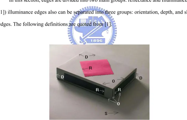
(18) which is a partial differential equation in Îout . Substituting F we obtain the following equation: ⎛ ∂ 2 Îout ∂G x − 2 ⎜⎜ 2 ∂x ⎝ ∂x. ⎞ ⎛ ∂ 2 Îout ∂G y − ⎟⎟ + 2 ⎜⎜ 2 ∂y ⎠ ⎝ ∂y. ⎞ ⎟⎟ = 0 ⎠. (2.14). Divided by 2 and rearranging terms, we obtain the well-known Poisson equation: ∇ 2 Îout = div G. where ∇ 2 is the Laplacian operator ∇ 2 Îout = gradient field G define as div G =. (2.15). ∂ 2 Îout ∂ 2 Îout + and div G is the divergence of the ∂x 2 ∂y 2. ∂G x ∂G y . + ∂y ∂x. In order to solve this problem, we could use the Full Multi-grid Algorithm [7], or the fast Fourier Transform to invert the Laplacian operator. Because this method is applied to the gray level image, we need to assign colors to the pixels of the image. Here, we transform RGB color space to HSI color space first, and then apply our algorithm on the I channel. Finally, transform back to the RGB color space use the original H, S, and new I channel.. 9.

(19) Chapter 3. Gradient attenuation function In this chapter, we first introduce types of edges, and how to distinguish illumination from reflectance edges. Finally, we propose our gradient attenuation function to reduce shadow and shading step by step.. 3.1. Types of edges In this section, edges are divided into two main groups: reflectance and Illuminance edges [1]) illuminance edges also can be separated into three groups: orientation, depth, and shadow edges. The following definitions are quoted from [1].. Figure 3.1 Types of Edges: orientation edges (O), depth edges (D), reflectance edges (R), and shadow edges (S).. Reflectance edges are changes in image luminance caused by changes in the reflectance. of two retinally adjacent surfaces. Reflectance edges can occur when the surfaces are made of different materials or painted different colors. Examples of reflectance edges in Figure 3.1 are 10.

(20) labeled with R’s. Illumination edges are changes in image luminance caused by different amounts of light. falling in a single surface of homogeneous reflectance. Illumination edges can be caused by cast shadows, reflected highlights on glossy, restricted spotlights (as in theater lighting), or changes in surface orientation. There are three kinds of illumination edges: Orientation edges refer to places in the environment in which there are. discontinuities in surface orientation. These occur when two surfaces at different orientations meet along an edge in the 3D world. They usually arise at internal edges within a single object (e.g., a cube) or where one object abuts another, such as a block sitting in a table. Examples of orientation edges in Figure 3.1 are labeled with O’s. Depth edges refer to places where there is a spatial discontinuity in depth between. surfaces, that is, places in the image where one surface occludes another that extends behind it, with space between the two surfaces. If they actually touch along the edge, then it is classified as a depth edge. Examples of orientation edges in Figure 3.1 are labeled with D’s. Shadow edges are formed where there is difference in the amount of light falling on. a homogeneous surface, such as the edge of shadow, highlight, or spotlight. Examples of illumination edges in Figure 3.1 are labeled with S’s. From Figure 3.1, we find that the lighting on the same surface is smoothing except causing shadow edges. In order to eliminate illuminance also means to attenuate orientation (O), depth (D), and shadow (S) edges, and to preserve reflectance (R) edges. The filter based tone mapping algorithm wants to separate illuminance and reflectance image under the logarithm domain. As explained in section 1.2, they assume that the illuminance image usually occupied the lower frequency. There fore, they stand the smoothing image as the illuminance image, and derive the reflectance image from dividing original image by illuminance image. But this smoothing image actually is different from the real illuminance image, although 11.

(21) the bilateral [17] and the trilateral filter [18] use additional property to preserve illuminance sharp edge. These ideas still cause the following trouble. If the sigma of the range filter is too small, than this formula also preserve unwanted reflectance edge. On the other hands, if the sigma of the range filter is too large, than this formula will eliminate the illuminance edge that we want to preserve. This is a trade-off between preserving the smaller illuminance edge and eliminating the larger reflectance edge.. 3.2. Distinguishing illuminance from reflectance edges In Stephen E. Palmer [1], there are several simple criteria to separate these edges which are quoted as follows:. Spectral Cross-points Present. Absent. r2. w1. # Photons. B r1. # Photons. Opposite Slope Sign. Present. A. w2. Wavelength. Wavelength. r1. # Photons. r2. w2. Wavelength. D. r1. # Photons. C Absent. r2. w1. w2. w1. r1. r2. w1. w2. Wavelength. Figure 3.2 The chromatic property proposed by Rubin and Richard [12].. The planarity. If depth in formation indicates that two regions are not coplanar, the edge. between them tends to be perceived as an illumination edge rather than a reflectance edge, even 12.

(22) if it is sharp rather than fuzzy. The reason is that surfaces at different depths and/or orientations usually receive different amounts of illumination because of the physical behavioral of light. The illuminance ratios. Illumination edges can produce much greater changes in. luminance than reflectance edges. A good white surface typically reflects no more than about 90% of the incident photons, and a good black surface reflects no less than about 10%. Reflectance ratios are therefore unlikely to be greater than about 10:1. But illumination ratio can be 1000:1 or more. Therefore, if a luminance ratio is 10:1 or more, a good heuristic is to assume that is due to a difference in illumination. Fuzzy or sharp edge. Illumination edges due to shadows or spotlights tend to be fuzzy. and some what graded, whereas reflectance edges tend to be sharp. In the absence of information to the contrary, the visual system tends to assume that a sharp edge between coplanar regions is a reflectance edge. The chromatic property. Color provides additional information for distinguishing. between illumination and reflectance edges. Intuitively, the crucial fact is that differences in illumination will almost always produce similar hue and saturation values on opposite sides of an edge, whereas differences in reflectance almost never will. Generally speaking, if hue or saturation varies across an edge, it is probably a reflectance edge. If only brightness varies, it probably an illumination edge. Besides, Rubin and Richard [12] provide another chromatic heuristics for discriminating between reflectance and illumination edges. They proposed two conditions that signify changes in spectral reflectance of surfaces: spectral cross-point and opposite slop signs. These conditions are defined by relations between the light reflected from the two regions of interest as sampled at two different wavelengths. The spectral cross-point condition is illustrated in Figure 3.2 A and C. It holds when the measurements in any two regions produce opposite differences in the amount of light at the two wavelengths, resulting in the “crossed” spectral graphs of Figure 3.2 A and C. The opposite slope sign condition is illustrated in Figure 3.2 A 13.

(23) and B. It holds when the slopes of the graphs of the two regions have different signs: one goes up and the other down. The fact that these two conditions are independent is demonstrated by the four graphs in Figure 3.2, each of which shows a different pairing of presence versus absence of the two conditions. Only the last condition (Figure 3.2 D), showing the absence of both, indicates a case in which the spectral difference between the two regions is likely to be due to an illumination edge. Here, we can not use the planarity information, because of the poor depth information from a single image. In order to preserve reflectance edges and attenuate illuminance edges, we construct a gradient attenuation function utilizing the other criterion step by step in the rest of the chapter.. 3.3. The illuminance ratios By the illuminance ratios information, Fattal et al. [8] designed a good gradient attenuation function to fit this criterion. Their idea is based on that any drastic change in the luminance across an image must give rise to large magnitude luminance gradients at some scale. Fine details, such as texture, correspond to gradients of much smaller magnitude at a fine scale. So they want to identify large gradients at various scales, and attenuate their magnitudes while keeping their direction unaltered. Thus the attenuation must be progressive, penalizing larger gradients more heavily than smaller ones, and compressing drastic luminance changes, while preserving fine details. Real-world images contain edges at multiple scales. Therefore, in order to detect all of the significant intensity transition, they use a multi-resolution edge detection scheme. Then they propose propagating the desired attenuation from the level it was detected at to the full resolution image to prevent the halo artifact. We outline the algorithm as follows: At first they construct a Gaussian pyramid Î0 ,K , Îd , where Î is the logarithm of the. 14.

(24) luminance of the image, Î0 is the full resolution HDR image and Îd is the coarsest level in the pyramid. d is chosen such that the width and the height of Îd are at least 32. At each level j we compute the gradients using central differences: ⎛ Î j ( x + 1, y ) − Î j ( x − 1, y ) Î j ( x, y + 1) − Î j ( x, y − 1) ⎞ , ∇Î j ( x, y ) = ⎜ ⎟ j+1 ⎜ ⎟ 2 2 j+1 ⎝ ⎠. (3.1). At each level j a scaling factor ϕÎ ( x, y ) is determined for each pixel based on the magnitude j. of the gradient there: ⎛ ∇Î j ( x, y ) ϕÎ ( x, y ) = ⎜ j ⎜ α ⎝. ⎞ ⎟ ⎟ ⎠. β−1. (3.2). where α determines the gradient magnitude at which the edge is modified differently. The gradient whose value is larger than α is attenuated (0< β< 1). The gradient whose value is smaller than α is magnified. They suggest setting α to 0.1 times the average gradient magnitude, and β between 0.8 and 0.9. The full resolution gradient attenuation function Φ Î (x , y ) is computed in a coarse-to-fine fashion by propagating the scaling factors ϕÎ ( x, y ) from each level to the next using linear j. interpolation and accumulating them using point-wise multiplication. The process is given by the following algorithm: Init j=d : Φ Î ( x, y ) = ϕÎ ( x, y ) d. d. end for j from d-1 to 0. ( ) ( x, y ) ϕ. Φ Î ( x, y ) = L Φ Î j. j+1. (3.3) Î j. ( x, y ). end Φ Î ( x, y ) = Φ Î ( x, y ) 0. where d is the coarsest level, Φ Î denotes the accumulated attenuation function at level j, and L j. 15.

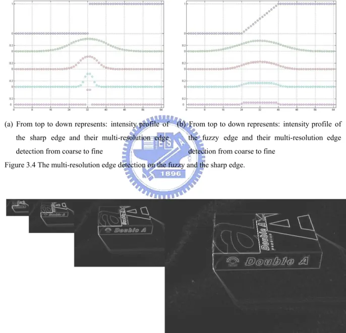
(25) is an up-sampling operator with linear interpolation. The gradient attenuation at each pixel of the finest level is determined by the strengths of all the edges (from different scales) passing through that location in the image. Using this multi-resolution scheme would attenuate the edges which are sharper, stronger, and coarser, and preserve the edges which are fuzzier, weaker, and thinner. Thus it could enhance the smaller texture. For the fuzzy edges (usually are shadow edges), it is not sufficient attenuated (see section 3.4 for detail). Because of the property of the fuzzy edge it has a stronger edge on the higher level (coarser level), and a weaker edge on a lower level (finer level). So the scaling factor on the higher level wants to attenuate more for the stronger edge, the scaling factor on the lower level wants to preserve for the weaker edge. Therefore, it could not reduce shadow edge. See Figure 3.3 for an example. In the next section, we modify this method to achieve our goal—reducing shadows by adding more criteria.. (b) The result of the gradient domain method [8]. (a) The original image. Figure 3.3 Result by Fattal et al [8]. The shadow is still there. T. 3.4. Fuzzy or sharp edge We know that the shadow edge is usually fuzzy, so we need to adjust the gradient of such edge. In our observation, the fuzzy edge usually can be found from the information available at two levels. There are four situations between the two levels: 16.

(26) 1. There is an edge at the coarser level, and it is also an edge at the finer level. 2. There is an edge at the coarser level, but it is no edge at the finer level. 3. There is no edge at the coarser level, but it is an edge at the finer level. 4. There is no edge at the coarser level, and there is also no edge at the finer level.. (a) From top to down represents: intensity profile of. (b) From top to down represents: intensity profile of. the sharp edge and their multi-resolution edge. the fuzzy edge and their multi-resolution edge. detection from coarse to fine. detection from coarse to fine. Figure 3.4 The multi-resolution edge detection on the fuzzy and the sharp edge.. Figure 3.5 The multi-resolution edge detection of the image in Figure 3.3 (a).. 17.

(27) (a) The gradient magnitude of the image in Figure 3.3 (a) at level 0. (b) The local standard deviation divided by the local mean (within a 5*5 window) of the left image. Figure 3.6 The local standard deviation divided by the local mean. T. In Figure 3.5 and Figure 3.4, we find that the sharp edge appears in each level, but the fuzzy edge only appears in the coarser level (situation 2). But only using this condition might create some problems, resulting in identifying the neighborhood of a sharper edge at the finer level as a fuzzy edge. In our experiment, the fuzzy edge also has the smaller local standard deviation than the sharper edge. If the local mean is larger, the local standard deviation needs to be larger to classify as the non-fuzzy edge. In Figure 3.6, we could see that the fuzzy edges have the smaller value. Under these observations, the fuzzy edge can be determined by Algorithm 3.1.. 18.

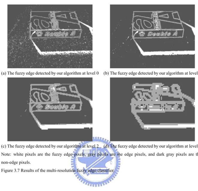
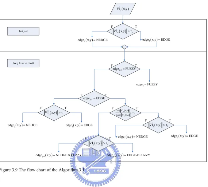
(28) Algorithm 3.1 Fuzzy edge classifier algorithm Init j=d: if ∇Î j ( x,y ) > τ1 , then edged ( x,y ) = EDGE else edged ( x,y ) = NEDGE end end for j from d-1 to 0 if edge j+1 ( x, y ) = FUZZY edge j ( x, y ) = FUZZY end if edge j+1 ( x, y ) = NEDGE if ∇Î j ( x,y ) > τ1 , then edge j ( x,y ) = EDGE else edge j ( x,y ) = NEDGE end else if. (. std ∇Î j ( x,y ). (. ). mean ∇Î j ( x,y ). ). > τ2. if ∇Î j ( x,y ) > τ1 , then edge j ( x,y ) = EDGE else edge j ( x,y ) = NEDGE end else edge j+1 ( x,y ) = FUZZY end end end. where d is the coarsest level, ∇Î j ( x, y ) is defined in (3.1), edge j ( x, y ) is the edge label at level j, std ( x ) is the local standard deviation, and mean ( x ) is the local mean. Figure 3.9 is the flow chart of this algorithm. The fuzzy edges that we detect by Algorithm 3.1 are shown in Figure 3.7.. 19.

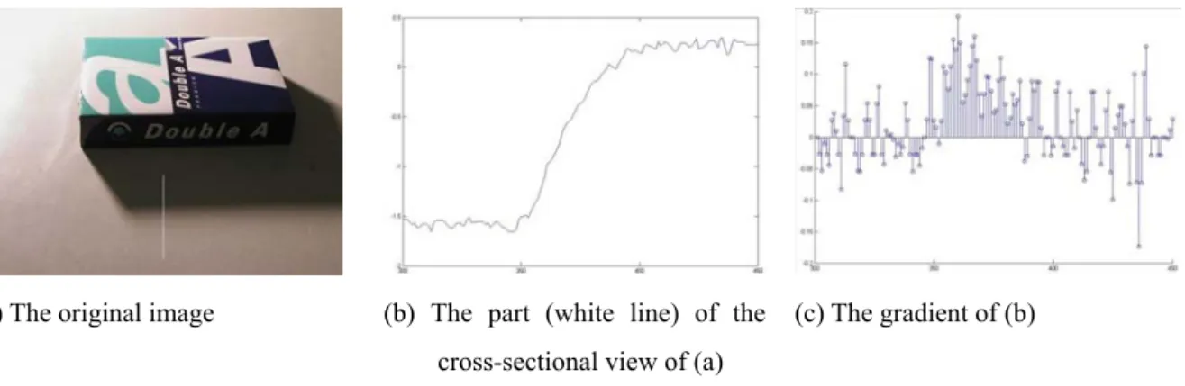
(29) (a) The fuzzy edge detected by our algorithm at level 0. (b) The fuzzy edge detected by our algorithm at level 1. (c) The fuzzy edge detected by our algorithm at level 2. (d) The fuzzy edge detected by our algorithm at level 3. Note: white pixels are the fuzzy edge pixels, gray pixels are the edge pixels, and dark gray pixels are the non-edge pixels. Figure 3.7 Results of the multi-resolution fuzzy edge classifier.. However, we could find that the texture information exists in the whole image. The most gradient value in the area of the fuzzy edges is either positive or negative. But, the gradient value in the area of the non-fuzzy edges alternate with positive and negative value uniformly. In Figure 3.8, we can find this phenomenon. The pixels between 300 and 350 are the shadow area, the pixels between 350 and 400 are the fuzzy edge, and the pixels between 400 and 450 are the bright area. We find that the gradient value between 350 and 400 almost are positive value, and the gradient value of the other area alternate with positive and negative value. Thus, if using the attenuation function proposed by Fattal et al. [8] cannot reduce shadow effect unless set the gradient value between 350 and 400 to 0 in order to let the shadow area reveal. The region of the fuzzy edge would be more and more blur, and it becomes the tradeoff between the shadow. 20.

(30) reduction and the texture information in the region of the fuzzy edges. Thus, in the region of the fuzzy edge, we propose subtracting the local mean of the gradient value from the gradient of that pixel. This method would let the distribution of the positive and the negative value in the area of the fuzzy edge more uniform. The algorithm to fix the gradient value in the area of the fuzzy edges is shown in Algorithm 3.2.. Algorithm 3.2 Gradient adjustment algorithm Init j from d to 0: offset j ( x, y ) = ( 0, 0 ) end for j from d-1 to 0 if edge j ( x, y ) = FUZZY. (. offset j ( x, y ) = ⎡⎣ L ( offset j+1 ) ( x, y ) ⎤⎦ + mean ∇Î j ( x, y ). ). end end offset ( x, y ) = offset 0 ( x, y ) / counter ( x, y ). where d is the coarsest level, ∇Î j ( x, y ) is defined in (3.1), edge j ( x, y ) is the edge label at level. j,. (. offset j ( x, y ). ). mean ∇Î j ( x,y ) =. is. the. gradient. offset. at. the. location. ( x, y ). ,. d ⎛⎢ x ⎥ ⎢ y ⎥⎞ ˆ I x+a,y+b ∇ counter x, y E j ⎜ ⎢ j ⎥ , ⎢ j ⎥ ⎟ , and , = ( ) ( ) ∑ j 2 ∑ ∑ j= 0 ⎝⎣2 ⎦ ⎣2 ⎦⎠ ( 2w + 1) a =− w b=− w. 1. w. w. ⎧1 ,if edge j ( x, y ) = FUZZY E j ( x, y ) = ⎨ . ⎩0 ,otherwise. 21.

(31) (a) The original image. (b) The part (white line) of the. (c) The gradient of (b). cross-sectional view of (a) Figure 3.8 Fuzzy edge profile and its gradient.. We simply add this decision into equation(3.2) , and rewrite it as follows: ⎛ ∇Î j ( x, y ) − OFFSETj ( x, y ) ϕÎ ( x, y ) = ⎜ j ⎜ α ⎝. ⎞ ⎟ ⎟ ⎠. β−1. (3.4). where ϕÎ ( x, y ) is the scale factor at each level j, α determines which gradient magnitudes j. remain unchanged. The gradient whose value is larger than α is attenuated (0< β< 1), and OFFSETj ( x, y ) is the Gaussian pyramid of the offset ( x, y ) . The attenuation function is the. same as equation(3.3). Finally, we could calculate the gradient field by the following equation:. (. ). G ( x, y ) = ∇Î ( x, y ) − offset ( x, y ) Φ Î ( x, y ) Using equation(2.15) we could reconstruct the image from the gradient field G.. 22. (3.5).

(32) ∇Î j ( x,y ). F Init j=d. ∇Îd ( x,y ) > τ1. T. edged ( x,y ) = EDGE. edged ( x,y ) = NEDGE. For j from d-1 to 0. F. T edge j+1 = FUZZY. edge j = FUZZY. F. F. edge j ( x,y ) = NEDGE. ∇Î j ( x,y ) > τ1. T edge j+1 = EDGE. T. F. (. std ∇Î j ( x,y ). (. ). mean ∇Î j ( x,y ). ∇Î j ( x,y ) > τ1. edge j+1 ( x,y ) = NEDGE & FUZZY. > τ2. F. edge j ( x,y ) = EDGE. F. T. ). T. ∇Î j ( x,y ) > τ1. edge j ( x,y ) = NEDGE. edge j+1 ( x,y ) = EDGE & FUZZY. Figure 3.9 The flow chart of the Algorithm 3.1. 23. T. edge j ( x,y ) = EDGE.

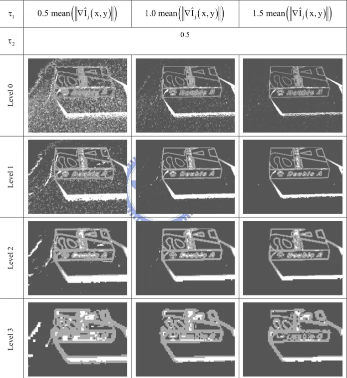
(33) Chapter 4. Experimental results In this chapter, we would discuss the parameters in our algorithm, and then we compare our algorithm with the other method. All the images are captured by the Olympus C4040Z at the resolution of the 640x480 pixels.. 4.1. Different parameter setting In this section, we would discuss the parameters in our method. These parameters can divide into two groups. τ1 and τ2 determine which edge would classify as the fuzzy edge. α and β determine which gradient should be enhanced and which gradient should be attenuated as described in section 3.3.. 4.1.1. The parameters of the edge classification algorithm These parameters would affect the classification of the fuzzy edges. If we fix τ2 , and adjust τ1 . In Table 4.1, the smaller τ1 , the more pixels we would classify as the edge in the coarse level (j+1). This would let the more fine level (j) pixels whose local standard deviation divide by local mean less than τ2 have more chance to become the fuzzy edges. If we fix τ1 , and adjust τ2 . In Table 4.2, the larger τ2 would let the more pixels whose coarser level is classified as the edge, become the fuzzy edges. In our experiment, we suggest setting τ1 about 0.5~1.0 times the average gradient magnitude, and τ2 between 0.4 and 0.5 (see Figure 4.1).. 24.

(34) Table 4.1 The results for different values of. τ1. (. 0.5 mean ∇Î j ( x, y ). ). τ1 .. (. 1.0 mean ∇Î j ( x, y ). ). (. 1.5 mean ∇Î j ( x, y ). ). 0.5. Level 3. Level 2. Level 1. Level 0. τ2. Note: white pixels are the fuzzy edge pixels, gray pixels are the edge pixels, and dark gray pixels are the non-edge pixels.. 25.

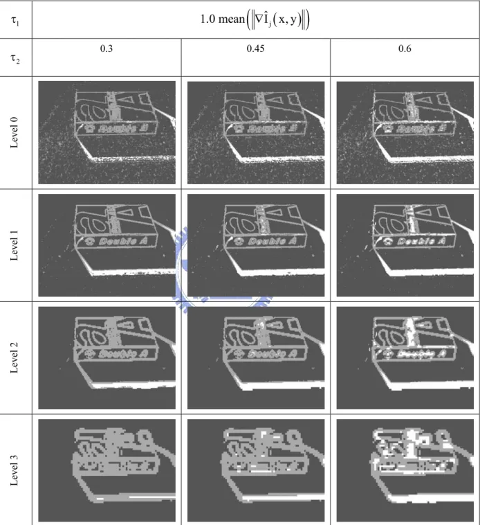
(35) Table 4.2 The results for different values of. (. 1.0 mean ∇Î j ( x, y ). τ1 0.3. 0.45. ) 0.6. Level 3. Level 2. Level 1. Level 0. τ2. τ2 .. Note: white pixels are the fuzzy edge pixels, gray pixels are the edge pixels, and dark gray pixels are the non-edge pixels.. 26.

(36) (a) The fuzzy edge detected by our algorithm at the level 0. (b) The fuzzy edge detected by our algorithm at the level 1. (c) The fuzzy edge detected by our algorithm at the level 2. (d) The fuzzy edge detected by our algorithm at the level 3. Note: white pixels are the fuzzy edge pixels, gray pixels are the edge pixels, and dark gray pixels are the non-edge pixels.. (. Figure 4.1 The results obtained with the suggested parameters ( τ1 = 1.0 mean ∇Î j ( x, y ). ), τ. 2. = 0.45 ).. 4.1.2. Adjustment of the gradient in the fuzzy area In this section, we verify our method that uses local mean to adjust the gradient in the fuzzy area would remove fuzzy edge in the image. We use our fuzzy edge classifier to detect fuzzy edge after adjustment the gradient in the fuzzy area. In Table 4.3, before adjustment, we can find lots of fuzzy edges (white pixels); after adjustment, the fuzzy edges are almost gone. Thus, our algorithm could remove the fuzzy edges that we detect.. 27.

(37) Table 4.3 The effect of adjustment of the gradient in the fuzzy area. After. Level 3. Level 2. Level 1. Level 0. Before. Note: white pixels are the fuzzy edge pixels, gray pixels are the edge pixels, and dark gray pixels are the non-edge pixels.. 28.

(38) 4.1.3. The parameters of the attenuation function These parameters would affect the attenuation function. If we fix β , and adjust α . In Table 4.4, the larger α would preserve the more fine detail. In other words, the attenuation function would be larger, and let both of the local and the global contrast larger. If we fix α , and adjust β . In Table 4.5, the smaller β would enhance small gradient more, and attenuate large gradient more. This would let the “contrast” of the attenuation function become larger, but this would make the contrast of the large gradient area smaller (more blur) and make the contrast of the small gradient area larger (sharper). In our experiment, we suggest setting α as 0.1~0.2 times the average gradient magnitude, and β between 0.8 and 0.9.. Table 4.4 The results for different values of α .. α. (. 0.1 mean ∇Î j ( x, y ). ). (. 0.5 mean ∇Î j ( x, y ). β. ). Result. Attenuation function. 0.9. Note: for the attenuation function, the darker pixel, the smaller attenuation value.. 29. (. 1.0 mean ∇Î j ( x, y ). ).

(39) Table 4.5 The results for different values of. α. β.. (. 0.1 mean ∇Î j ( x, y ). β. 0.8. 0.9. Result. Attenuation function. 0.7. ). Note: for the attenuation function, the darker pixel, the smaller attenuation value.. The shadow removal method proposed in this thesis suffers from some problems. First, as describe in section 3.4, the gradient which subtracts its local mean could remove the shadow, and preserve the detail in the fuzzy edge area, but this method still make a little blur in the fuzzy edge area. If we classify the fuzzy edge again after adjustment the fuzzy edge area, the fuzzy edges still reveal. Second, the shadow removal method is only dealing with the intensity, and we don’t take the color information for further processing. Because the color information inside the shadow region is severely destroyed, the color in this region is not the same as that in the normal lighting environment. We also notice that if the intensity inside the shadow region is too small, the “color shift” will be much worse. For this reason, the shadow removal method performs better under the condition when the contrast between the light and shadow region is small, i.e. the color information in the shadow region is still preserved. This is the main problem of our method, and can be improved by considering the color information. 30.

(40) Finally, because the shadow removal method performs the subtraction of local mean before attenuation, the “halo affect” will arise. However, it is not quite appearant under the normal condition, except for the sharper edge area. Thus, we can simply ignore the affect. Table 4.6 shows more results obtained by our method for a variety of images. In general, our method is capable of removing the shadow. However, as mention above, our method suffers from two effects: blurring and some color shift.. Table 4.6 Results by our method. Although there are some problems discussed in section 4.1, the shadow is almost gone. Original image. Results by our method. 31.

(41) Table 4.6 (continued) Original image. Results by our method. 32.

(42) Table 4.6 (continued) Original image. Results by our method. 4.2. Comparison with the other methods We compare our method with the other methods, such as histogram equalization, Fattal et al. method [8], unilateral [16], and bilateral filter [17]. We use the pictures in Figure 4.2 as the input images. We use the pictures to test whether the texture under the shadow is preserved or not. In Figure 4.3 (a), the histogram equalization enhances the contrast in the bottom left area, but it also reduces the contrast in the other area. In Figure 4.3 (b), it enhances the contrast in the upper half, but it also reduces the contrast in the dark shadow area. In Figure 4.4 (a), the unilateral filter reduces the shadow slightly, but still reveals, and enhances the detail in the dark area such as the trees on the both sides. In Figure 4.4 (b), it also reduces shadow slightly, and enhances the detail in the shadow area. In Figure 4.5 (a), the bilateral filter reduces the shadow effect stronger than the unilateral filter, but it removes some texture information such as the. 33.

(43) lawn and the leaves in the whole image. In Figure 4.5 (b), it removes shadow better than unilateral filter, but it also removes some texture information in the whole image. In Figure 4.6, the Fattal et al. method reveals the detail information in the dark area, as well as the shadow area, but the shadow still exists. It is because the fuzzy edge property described in section 3.4. In Figure 4.7, our method extends Fattal et al. work, thus we have the advantage of the Fattal et al. method, and removes the “fuzzy” shadow, too. However, the whole image becomes blurring slightly (see Table 4.6 for more examples).. 34.

(44) (a). (b) Figure 4.2 Original images.. 35.

(45) (a). (b) Figure 4.3 Results by Histogram Equalization.. 36.

(46) (a). (b) Figure 4.4 Results by Unilateral Filter.. 37.

(47) (a). (b) Figure 4.5 Results by Bilateral Filter.. 38.

(48) (a). (b) Figure 4.6 Results by Fattal’s method.. 39.

(49) (a). (b) Figure 4.7 Results by Our method.. 40.

(50) Chapter 5. Conclusion and future work 5.1. Conclusion In this thesis, we modify Fattal et al. algorithm which is originally used in the tone-reproduction for the high dynamic-range image, and if can also be applied to the shadow removal. The original method doesn’t produce the satisfying results because of the blurring affect, so we first detect the fuzzy edges by the multi-resolution approach, and then subtract the local means of the gradients within those regions. This modification reduces the blurring affect very well, but there still have many improvements for us to work out. How do we adjust the gradients within the fuzzy edge? Is it suitable to simply subtract the local-mean without the consideration of the noise? The fuzzy edge detection is also the important step which can influence the performance severely. In our knowledge of the “fuzzy edge” detection, the way is using the multi-resolution to detect the possible fuzzy edges. Besides, we use the “binary” edge detection approach to decide whether the specific position in the image is fuzzy edge or not, the approach may be extends to the “fuzzy” edge detection by applying the fuzzy set. However, we can not ensure affirmly whether the detection method can be used in the generalized case, and whether the percentage of the correct fuzzy edge detection fulfills our requirements? So, we still have more experiments to do to confirm the correctness of the detection method. The “color shift” is another challenge in the shadow removal. It’s not enough to deal with the shadowing images by only considering the intensity information. Instead, the color information should be included in the consideration in order to correct the problem of “color shift“.. 41.

(51) 5.2. Future work We adopt the concept of gradient domain to deal with the shadow removal problem. The concept of the attenuation in gradient domain can also be migrated to the wavelet domain because the HH, LH, HL sub-bands after the high-pass filter also represent the higher frequency of the original image, which is the same as the gradient indicates. Maybe we can apply our shadow removal method to the wavelet domain. In addition, our shadow removal method still leaks the chromatic information, which causes the problem of “color shift“. We have found that the illumination-invariant approach may be overcome this problem, however, due to the limit of time, we expect to correct the color shift in the future. If the chromatic information is included, not only fuzzy edges but the sharp edges can also be detected correctly, this enhancement will then fulfill the requirement of the shadow removal.. 42.

(52) References [1] Stephen E. Palmer, Vision science: photons to phenomenology, MIT Press, Cambridge, 1999. [2] Debevec, P. E. and Malik, J., “Recovering high dynamic range radiance maps from photographs”, In Proc. ACM SIGGRAPH, pp.369–378, 1997. [3] T. Mitsunaga and S. K. Nayar, “Radiometric Self Calibration”, Proc. of IEEE Conference on CVPR, Fort Collins, June 1999. [4] M. D. Grossberg and S. K. Nayar, “High Dynamic Range from Multiple Images: Which Exposures to Combine?”, In Proc. ICCV Workshop on Color and Photometric Methods in Computer Vision, Nice, France, October 2003. [5] S. K. Nayar and T. Mitsunaga, “High Dynamic Range Imaging: Spatially Varying Pixel Exposures”, Proc. of IEEE Conference on CVPR, Hilton Head Island, South Carolina, June 2000. [6] S. K. Nayar and V. Branzoi, “Adaptive Dynamic Range Imaging: Optical Control of Pixel Exposures Over Space and Time”, In Proc. ICCV, Nice, France, October 2003. [7] Press, W. H., Teukolsky, S. A., Vetterling, W. T., and Flannery, B. P., Numerical Recipes in C: The Art of Scientific Computing, 2nd edition, Cambridge University Press, 1992. [8] R. Fattal, D. Lischinski, and M.Werman, “Gradient domain high dynamic range compression”, Proc. of SIGGRAPH, pp.249–356, July 2002. [9] Tumblin, J., and Rushmeier, H. E., “Tone reproduction for realistic images”, IEEE Computer Graphics and Applications 13, 6, pp.42–48, November 1993. [10] M.F. Tappen, W.T. Freeman, and E.H. Adelson, “Recovering Intrinsic Images from a Single Image”, Proc. of Neural Information Processing Systems, 2002. [11] Y. Weiss, “Deriving intrinsic images from image sequences”, In Proc. ICCV, Vol. 2, pp.68-75, 2001. [12] J.M. Rubin and W.A. Richards, “Color vision and image intensities: When are changes material?” , Biol. Cybern., vol. 45, no. 3, pp.215–226, 1982. [13] Perona, P., and Malik, J., “Scale-space and edge detection using anisotropic diffusion.”, IEEE Transactions on PAMI 12, 7 , pp.629–639, July 1990 [14] Ruifeng Xu, and Sumanta N. Pattanaik, “High Dynamic Range Image Display Using Level Set Framework.”, 2003 [15] Tumblin, J., and Turk, G., “LCIS: A boundary hierarchy for detail-preserving contrast reduction”, In Proc. ACM SIGGRAPH, pp.83–90, 1999. 43.

(53) [16] Jobson, D. J., Rahman, Z., and Woodell, G. A., “A multi-scale Retinex for bridging the gap between color images and the human observation of scenes”, IEEE Transactions on Image Processing 6, 7, pp.965–976, July 1997 [17] Frédo Durand, and Julie Dorsey, “Fast bilateral filtering for the display of high dynamic range images”, ACM Transactions on Graphics, v.21 n.3, July 2002 [18] Choudhury P, and Tumblin J., “The trilateral filter for high contrast images and meshes”, In Proceedings of the Eurographics Symposium on Rendering, pp.186–96, 2003 [19] Stockham, J. T. G., “Image processing in the context of a visual model.”, In Proc. of the IEEE, vol. 60, pp.828–842, 1972. [20] Pattanaik, S. N., Ferwerda, J. A., Fairchild, M. D., and Greenberg, D. P., “A multi-scale model of adaptation and spatial vision for realistic image display.”, In Proc. ACM SIGGRAPH, pp.287–298, 1998. [21] Dicarlo, J. M., and Wandell, B. A., “Rendering high dynamic range images”, In Proc. of the SPIE: Image Sensors, vol. 3965, pp.392–401, 2001 [22] Masashi Baba and Naoki Asada, “Shadow removal from a real picture”, Proc. of the SIGGRAPH conference on Sketches & applications: in conjunction with the 30th annual conference on Computer graphics and interactive techniques, pp.27-31, San Diego, California, July 2003 [23] A. Koschan and M. Abidi, “Detection and Classification of Edges in Color Images”, Signal Processing Magazine, Special Issue on Color Image Processing, Vol. 22, No. 1, pp.64-73, 2005 [24] Graham D. Finlayson, Mark S. Drew, and Cheng Lu, “Intrinsic Images by Entropy Minimization”, ECCV, Vol. 3023, pp. 582-595, 2004 [25] Y. C. Chung, J. M. Wang, R. R. Bailey, S. W. Chen, S. L. Chang, and S. Cherng, “Physics-based Extraction of Intrinsic Images from a Single Image”, 17th ICPR, Vol. 4, pp.693-696, August 2004. [26] Rafael C. Gonzalez, and Richard E. Woods, Digital Image Processing, 2nd edition, Prentice Hall press, 2002. [27] Ashikhmin, M., “A Tone Mapping Algorithm for High Contrast Images”, The Proc. of 13th Eurographics Workshop on Rendering, pp.145-155, 2002. [28] J. M. Geusebroek, R. van den Boomgaard, A. W. M. Smeulders, and H. Geerts, “Color invariance.”, IEEE Transactions on PAMI, vol. 23, no. 12, pp.1338–1350, 2001.. 44.

(54)