合作式通訊下以多輸入多輸出和正交分頻多工之接收端對抗多重頻率偏移

(1)

國立交通大學

電子工程學系電子研究所碩士班

碩

士論文

合作式通訊下以多輸入多輸出和正交分頻多工之接收端對抗

多重頻率偏移

A MIMO-OFDM Receiver to Combat Multiple Frequency Offsets in

Cooperative Communication

研究生 : 李俊育

指導老師 : 桑梓賢教授

(2)

合作式通訊下以多輸入多輸出和正交分頻多工之接收端對抗

多重頻率偏移

A MIMO-OFDM Receiver to Combat Multiple Frequency Offsets

in Cooperative Communication

研究生 : 李俊育 Student : Jyun-Yu Lee

指導教授 : 桑梓賢教授 Advisor : Tzu-Hsien Sang

國立交通大學

電子工程學系電子研究所碩士班

碩士論文

A Thesis

Submitted to Department of Electronics Engineering & Institute of Electronics College of Electrical and Computer Engineering

National Chiao Tung University in Partial Fulfillment of the Requirements

for the Degree of Master of Science

in

Electronics Engineering February 2011

Hsinchu, Taiwan, Republic of China

(3)

合作式通訊下以多輸入多輸出和正交分頻多工之接收端對

抗多重頻率偏移

研究生：李俊育指導教授：桑梓賢教授

國立交通大學

電子工程學系

電子研究所碩士班

摘要

在合作式通訊下，同步是一個很重要的議題，不像傳統的多輸入多輸出(MIMO)系統，合作式的天線是分屬於不同的中繼端，因此，對目的端而言，很難同時補償多重頻率偏移(MCFOs)，另外，傳統的空頻區塊碼在這邊可能不是很適用，在這篇論文裡，我們考慮從中繼端到目的端的通道是頻率選擇性衰減通道，提出的方法是結合兩個已分別做完同步的訊號來消除載波間干擾(ICI)，疊代式干擾消除被進一步用來獲得良好的位元錯誤率以及對於多重頻率偏移有更好的容忍度。關鍵字: 空頻區塊碼、正交分頻多工、合作式通訊、多重載波偏移、疊代式消除

(4)

A MIMO-OFDM Receiver to Combat Multiple Frequency

Offsets in Cooperative Communication

Student：Jyun-Yu Lee Advisor：Tzu-Hsien Sang

Department of Electronics Engineering & Institute of Electronics

National Chiao Tung University

ABSTRACT

Synchronization is an important issue in cooperative communications. Unlike in conventional MIMO systems, the cooperative antennas belong to different relay nodes. Therefore, it is hard for the destination node to compensate multiple carrier frequency offsets (MCFOs) simultaneously and the conventional space-frequency decoding may not be suited here. In this paper, we consider the cooperative transmission with MCFOs when the channels from relay nodes to the destination node are frequency selective fading. The proposed strategy which takes cues from literature [9] combines two sets of separately synchronized signal to mitigate inter-carrier interference (ICI). Iterative interference cancellation is deployed to further improve performance and tolerance of MCFOs.

Keywords — SFBC, OFDM, cooperative communication, multiple frequency offsets,

(5)

誌

謝

首先，在這歷史性的一刻，讓我們慶祝中華民國一百年生日快樂，接著感謝指導教授桑梓賢博士，在碩士生涯裡給予我研究和課業上的幫助，不時的討論並指引我正確的方向，使我在這兩年多來獲益匪淺。韶光似箭，光陰荏苒，兩年多來的碩士生活，確實過的很紮實，對研究生而言，是沒有在放假的啦，尤其在碩一時，一方面要修課，一方面還要做計劃的東西，對剛進研究所的我來說實在很累又很無助，真的是蠟燭兩頭燒阿，往往在心情低落的時候，學長總是會安慰並鼓勵我，然後跟我說” 你的人生都走到這一步了，再撐一下不行嗎?當你想要放棄這文憑的時候，你看你背後有多少人想進來都還進不來阿，你想想你的父母這麼辛苦是為了什麼阿”，這些話總是對我當頭棒喝，這些話總是點醒了我，所以我就這樣一路走了過來，現在回想起來，宅在實驗室的兩個寒暑假裡，品嚐酸甜苦辣的滋味，這些點點低低，都將成為我永存的回憶。另外感謝在研究上給予我幫助的正湟學長、欣德學長，感謝每日與我朝夕相處的伙伴耀賢和旭謙以及學弟妹們，愛打三國的建宏、愛看NBA的建志、愛打羽球的柔綾、愛玩PS3的胤宏、愛打星海2的碩文，你們的歡笑聲和熱情，總是舒緩我做研究的苦悶，另外感謝commlab這個大家庭的所有成員，謝謝你們的照顧。最後，我要感謝我的家人，雖然相處的時間很少，但總是在背後給予我莫大的支持與鼓勵，沒有你們就沒有現在的我，謹以此論文獻給我的家人。李俊育謹誌 2011年2月

(6)

List of Figures

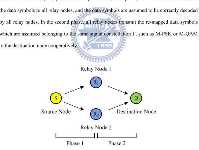
Fig. 2.1 A simple cooperative communication system model. ... 3

Fig. 3.1 The block diagram of the receiver with proposed MCFOs mitigation algorithm. ... 9

Fig. 3.2 A magnitude of the channel HA when |ε_R₁−ε_R₂| 0= ... 12

Fig. 3.3 A magnitude of the channel HB when |ε_R₁−ε_R₂| 0= ... 12

Fig. 3.4 A magnitude of the channel HA when |ε_R₁−ε_R₂| 0.4= ... 13

Fig. 3.5 A magnitude of the channel HB when |ε_R₁−ε_R₂| 0.4= ... 13

Fig. 3.6 A magnitude of the channel HA when |ε_R₁−ε_R₂| 0.8= ... 14

Fig. 3.7 A magnitude of the channel HB when |ε_R₁−ε_R₂| 0.8= ... 14

Fig. 3.8 Comparison of BER performance in the case of relative CFO = 0.8. ... 17

Fig. 3.9 Comparison of BER performance with different MCFOs. ... 18

Fig. 3.10 BER performance vs. relative CFO |ε_R₁−ε_R₂|. ... 18

Fig. 4.1 MLSE based detection utilizing Viterbi algorithm with QPSK ... 21

Fig. 4.3 The magnitude of 50th row of H1,w when K = 0 ... 23

Fig. 4.4 The magnitude of 50th row of H2 when K = 0 ... 24

Fig. 4.6 The magnitude of 50th row of H1 when K =1 ... 25

Fig. 4.8 The magnitude of 50th row of H2 when K = 1 ... 26

Fig.5.1 A cooperative communication system model in SM case. ... 27

Fig.5.2 The channel matrix of SM when |ε_R₁−ε_R₂| 0= . ... 30

Fig.5.4 The channel matrix of SM when |ε_R₁−ε_R₂| 2= . ... 31

Fig. 5.6 The magnitude of 50th row of H at K = 1 ... 32

(8)

List of Tables

TABLE 3.1 The value of C in different related CFO case ... 11

TABLE 3.2 Simulation Parameter ... 17

TABLE 4.1 SINR gain in different K value in SD case ... 22

(9)

Chapter 1 Introduction

In recent years, cooperative communication has drawn much attention in the field of wireless communication. The advantage of cooperative communication is that multiple single-antenna transceivers can share their antennas to create a virtual antenna structure. Therefore, the multiple-input multiple-output (MIMO) techniques, such as Alamouti’s space-time block coding (STBC), can be generalized for the distributed environment. Spatial diversity can be employed in such environment [2].

However, unlike in conventional MIMO systems, the cooperative antennas belong to different relay nodes which have different local oscillators and Doppler spreads and may not be either frequency or time synchronized, i.e., there exist multiple symbol timing offsets (MSTOs) and multiple carrier frequency offsets (MCFOs). Therefore, it is hard for the destination node to compensate either MSTOs or MCFOs simultaneously. In this paper, we mainly focus on the MCFOs compensation.

Many methods have been proposed in the literature to mitigate the MCFOs problem to cancel the inter-carrier interference (ICI) as follows. For instance, equalization schemes have been proposed to combat the MCFOs [3] [4]. However, these methods have high complexity in inverting matrices. In [5], several data detection and complexity-reducing methods are compared. In [6], an ICI-self cancellation scheme is proposed with a price of lowing transmission rate. In [7], a two-branch receiver structure is proposed. A two-step cancellation

(10)

procedure which is based on the inter-carrier interference (ICI) cancellation is proposed in [8]. A modified scheme which combines [7] and [8] is proposed in [9]. However, most of the techniques are only effective in a quite limited range of MCFOs and the performance would degrade significantly as the magnitudes of the MCFOs exceed the range.

In this thesis, we consider the cooperative communication for frequency selective fading channels with the MCFOs. The separate synchronizing scheme and a modified SFBC decoding technique in [9] are further improved. Iterative interference cancellation is also added to enhance the performance. The new receiver has a superior tolerance range of MCFOs and may be suitable for applications in asynchronous cooperative OFDM systems. As an alternative, the newly emerging technique of exploiting the covariance structure of residual ICI in [20] is also studied for combating MCFOs in both cases of Alamouti coding and spatial multiplexing.

The rest of this thesis is organized as follows. In Chapter 2, the system model is described. In Chapter 3, two branch MCFOs cancellation for Alamouti decoding is used. In Chapter 4, a MLSE with noise whitening is used for Alamouti decoding. In Chapter 5, an MLSE with noise whitening is used in spatial multiplexing. The conclusions are given in Chapter 6.

Notations: Superscripts (.)*, (.)T represents conjugate, transpose, respectively. ||.||, E[.] denote the norm and the expectation, respectively. And v(k) represents the k-th element in the vector v.

(11)

Chapter 2 System Model

A cooperative communication system with one source node, two relay nodes, and one destination node in this paper is shown in Fig. 2.1. Each node has only one antenna and the decode-and-forward (DF) protocol is adopted. In the first phase, the source node broadcasts the data symbols to all relay nodes, and the data symbols are assumed to be correctly decoded by all relay nodes. In the second phase, all relay nodes transmit the re-mapped data symbols which are assumed belonging to the same signal constellation Γ, such as M-PSK or M-QAM to the destination node cooperatively.

(12)

2.1 SFBC-OFDM

A SFBC-OFDM system is employed at the relay nodes. The data symbol vector

0 1 2 1

= ⎡_⎣X X X_N₋ X_N₋ ⎤_⎦T

X L is encoded into two vectors as

* * * 0 1 1 2 1 * * * 1 0 1 1 2 = = T k k N N T k k N N X X X X X X X X X X X X + − − + − − ⎡ − − − ⎤ ⎣ ⎦ ⎡ ⎤ ⎣ ⎦ R1 R2 X X L L L L (2.1),

where XR1 is transmitted from relay node 1, XR2 is transmitted from relay node 2 and k

is the subcarrier index. Then the transmitted signal xα(n) is derived from the inverse fast

Fourier Transform (IFFT) of the encoded data symbol Xα(k), α∈{R1,R2} , which can be

written as 1 0 1 2 ( ) N ( ) exp( ) , _p 1 k j nk x n X k N n N N N α α π − = =

∑

− ≤ ≤ − (2.2),

where N is the OFDM symbol length,N is the length of cyclic prefix (CP). _p

2.2 Received Signal with Multiple CFOs

Due to different oscillators, time invarying multipath channel models are assumed. The

discrete-time model of the received signals at the destination node after removing the CP can be written as 1 2 1 { , } 0 2 ( ) exp( )L ( ) ( ) ( ) R R l j n y n h l x n l z n N α α α α πε − ∈ = =

∑

− + (2.3),

(13)

where ε , _α α∈{ , }R R₁ ₂ is the normalized frequency offset given by F f α α ε = Δ Δ , ΔFα

is the frequency offset between the relay node α and the destination node, fΔ is the

subcarrier bandwidth of the SFBC-OFDM system. The h lα( ) represents the channel impulse

response (CIR) of the _{l tap,}th _{L is the number of multipath. ( )}

w n is the complex additive

white Gaussian noise (AWGN) with zero mean and variance _σ2_{. In order to avoid}

inter-symbol interference (ISI),N_p ≥ should be satisfied. The average total power is L

normalized such that

1 2 2 1 { , } 0 [ _{R R} L_l | ( ) | ] 1 E

∑

_α_∈

∑

₌− h l_α = .

In frequency domain, the received signals on two adjacent subcarriers are

1 2 1 2 1 2 1 2 0 1, 0 2, 1 1 1 , 1, 1, , 2, 2, 0 0 1 0 1, 1 1 0 2, 1 1 1 1, 1, 1, 1, 2, 2, 0 0 1 1 1 ( ) R R R R R R R R k R k k R k k N N k m R m R m k m R m R m m m m k m k k k R k k R k k N N k m R m R m k m R m R m m m m k m k k Y G H X G H X G H X G H X W Y G H X G H X G H X G H X W ε ε ε ε ε ε ε ε + − − = = ≠ ≠ ∗ ∗ + + + + − − + + = = ≠ + ≠ + + = + + + + = − + + + +

∑

(2.4),

where Hα, α∈{R1,R2}, is the channel frequency response and W is complex AWGN in

the frequency domain. G_{k m}ε_,α

is the ICI coefficient, which destroys orthogonality between sub-carriers, caused by multiple CFOs. It can be defined as

1 , 0 2 ( ) 1 exp( ) sin( ( )) 1 exp( ( )( )) sin( ( ) / ) N k m n j n k m G N N m k N j m k N m k N N α ε α α α α π ε π ε _π _ε π ε − = − + = − + − = − + − +

∑

(2.5),

(14)

When k = m, G_{k m}ε_,α _{can be simply defined as}

0

Gεα _{. Then we rewrite (2.4) into vector form}

as follows. εR1 εR2 R1 R1 R2 R2 Y = G H X + G H X + W (2.6), where ,0 ,1 , 1 0 0,1 0, 1 1,0 0 1, 1 1 2 1,0 1,1 0 0 0 0 0 , 0 0 , { , } N N N N N H H H G G G G G G R R G G G α α α α α α α α α α α α ε ε ε ε ε ε ε ε ε α − − − − − ⎡ ⎤ ⎢ ⎥ ⎢ ⎥ =_⎢ _⎥ ⎢ ⎥ ⎣ ⎦ ⎡ ⎤ ⎢ ⎥ ⎢ ⎥ =_⎢ _⎥ ∈ ⎢ ⎥ ⎢ ⎥ ⎣ ⎦ α α ε H G L L M M O M L L L M M O M L

Finally, perfect Channel State Information (CSI) which is known at destination node is assumed.

(15)

Chapter 3 Two-Branch MCFOs Cancellation for

Alamouti Decoding

A two-branch cancellation algorithm for SFBC-OFDM and multiple CFOs compensation is proposed. This algorithm is a further development of that in [9]. The method is designed for SFBC decoding in asynchronous cooperative systems by combining separately synchronized signal to extend the tolerance range of multiple CFOs. More details are described in the following.

3.1 Multiple CFOs Mitigation Algorithm

3.1.1 Separate Synchronization

As in [13], consider that the receiver can estimate individual CFO effectively and have multiple copies of the received signal compensated for different CFOs. For example, preambles which are orthogonal to each other for each relay node may be used to facilitate the estimation of CFOs. Before DFT, the compensated signal can be express as

( ) exp( 2 ) ( )

(16)

where 0 ≤ n ≤ N-1 and α∈{R1,R2}. Then, the two sets of separately synchronized signal

in the frequency domain can be written as Y n%_R₁( )=DFT y n

{

_%_R₁( )

}

and Y%_R₂( )n =DFT y

{

_%_R₂( )n

}

and we rewrite it into vector form as follows.

R1 R2 R1 R2 R1 R2 ε H ε ε H R1 R1 R1 R2 R2 R1 R1 R2 R2 R1 ε H ε ε H R2 R1 R1 R2 R2 H R1 R1 R2 R2 R2 Y = H X + (G ) G H X + (G ) W = H X + GH X + W Y = (G ) G H X + H X + (G ) W = G H X + H X + W (3.2), Let G = (G ) GεR1 H εR2, G is circular matrix, and it can be arranged as follows

−

+ −

−

*

R1,e R1,e e A R2,e o B R2,o e R1,e

* *

R1,o R1,o o C R2,o e D R2,e o R1,o

H H *

R2,e R2,e o A R1,e e D R1,o o R2,e

* H * H

R2,o R2,o e C R1,o o B R1,e e R2,o

Y = H X + G H X + G H X + W Y = H X + G H X + G H X + W Y = H X G H X G H X + W Y = H X G H X + G H X + W (3.3), where 0,0 0,2 0, 2 0,1 0,3 0, 1 2,0 2,2 2, 2 2,1 2,3 2, 1 2,0 2,2 2, 2 2,1 2,3 2, 1 1,1 1,3 1, 1 3,1 3,3 3, 1 1,1 1,3 1, , N N N N B N N N N N N N N N N N N N G G G G G G G G G G G G G G G G G G G G G G G G G G G − − − − − − − − − − − − − − − − − ⎡ ⎤ ⎡ ⎤ ⎢ ⎥ ⎢ ⎥ ⎢ ⎥ ⎢ ⎥ =_⎢ _⎥ =_⎢ _⎥ ⎢ ⎥ ⎢ ⎥ ⎢ ⎥ ⎢ ⎥ ⎣ ⎦ ⎣ ⎦ = A C G G G L L L L M M O M M M O M L L L L M M O M L 1,0 1,2 1, 2 3,0 3,2 3, 2 1 1,0 1,2 1, 2 , N N D N N N N N G G G G G G G G G − − − − − − − ⎡ ⎤ ⎡ ⎤ ⎢ ⎥ ⎢ ⎥ ⎢ ⎥ ₌⎢ ⎥ ⎢ ⎥ ⎢ ⎥ ⎢ ⎥ ⎢ ⎥ ⎢ ⎥ ⎢ ⎥ ⎣ ⎦ ⎣ ⎦ G L L M M O M L

[

X0 X2 XN−3 XN−1

]

,

[

X1 X3 XN−2 XN

]

= = e o X _L X _L A B C D A

: 1. G ,G ,G ,G all are circular matrices 2. G G

note

(17)

3.1.2 SFBC Decoding

The SFBC decoding algorithm is modified from [7] while the major difference is that our algorithm processes two sets of separately synchronized signal jointly, inspired by the method found in [10]. We compose two available sets of received signal, i.e. For the first branch, the

input vector is ⎡_⎣ * ⎤_⎦T

R1,e R2,o

Y Y . For the second branch, the input vector is ⎡_⎣ ₂ *₁ ⎤_⎦T

R ,e R ,o

Y Y .

Therefore, the signal after combiner can be written as follows and the block diagram is

illustrated in Fig. 3.1. ⎡ ⎤ ⎡ ⎤ ⎡ ⎤ ⎢ ⎥ ⎢ ₋ ⎥ ⎢ ⎥ ⎣ ⎦ ⎣ ⎦ ⎣ ⎦ ⎡ ⎤ ⎡ ⎤ ⎡ ⎤ ⎢ ⎥ ⎢ ⎥ ₋ ⎢ ⎥ ⎣ ⎦ ⎣ ⎦ ⎣ ⎦ H 1

R1,e A R2,e R1,e e

* T * *

1

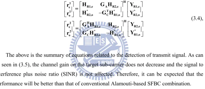
R2,o C R1,o R2,o o H H 2 R2,e A R1,e R2,e e * * * * 2 R1,o C R2,o R1,o o H G H Y r = H G H Y r Y G H H r = Y G H H r (3.4),

The above is the summary of equations related to the detection of transmit signal. As can be seen in (3.5), the channel gain on the target sub-carrier does not decrease and the signal to interference plus noise ratio (SINR) is not affected. Therefore, it can be expected that the performance will be better than that of conventional Alamouti-based SFBC combination.

1 e r 2 o r

(18)

(

)

(

)

(

)

(

)

(

)

(

)

1 I − + − 1 2 2 e R1,e R2,o e H T *

R1,e A R2,e R2,o C R1,o o

H T * *

R1,e B R2,o R2,o B R1,e e

H *

R1,e R1,e R2,o R2,o

2 2

R1,e R2,o e

1 H H * T *

o R2,e A A R2,e R1,o C C R1,o o

H H *

R2,e A R1,e R1,o C R2 r = | H | + | H | X + H G H H G H X + H G H + H G H X + H W + H W = | H | + | H | X + r = H G G H H G G H X + H

(

G H H G H

)

(

)

(

)

(

)

(

)

(

)

2 2 2 2 I | | I C − − + + = + + − * ,o e H H * T * *

R2,e A B R2,o R1,o C B R1,e e

H H * *

R2,e A R1,e R2,o C R2,o

H H * T *

R2,e A A R2,e R1,o C C R1,o o R2,e R1,o o

2 H H T * *

e R1,e A A R1,e R2,o C C R2,o e

H T

R1,e A R2,e R2,o C

X + H G G H H G G H X + H G W H G W = H G G H H G G H X H | H | X r = H G G H + H G G H X + H

(

G H H G

)

(

)

(

)

(

)

(

)

(

)

(

)

3 2 2 3 I | | | | I C − = = + + − − * R1,o o H H T * * *

R1,e A D R1,o R2,o C D R2,e o

H T *

R1,e A R2,e R2,o C R1,o

H H T * *

R1,e A A R1,e R2,o C C R2,o e R1,e R2,o e

2 2 2

o R2,e R1,o o

H H * *

R2,e A R1,e R1,o C R2,o e R2, H X + H G G H + H G G H X + H G W + H G W H G G H + H G G H X + H H X r = | H | + | H | X + H G H H G H X H

(

)

(

)

(

)

I4 − = + H H * * *

e D R1,o R1,o D R2,e o

H *

R2,e R2,e R1,o R1,o

2 2 R2,e R1,o o G H + H G H X + H W H W | H | + | H | X (3.5),

(19)

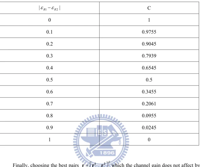
TABLE 3.1 The value of C in different related CFO case 1 2 |ε_R −ε_R | C 0 1 0.1 0.9755 0.2 0.9045 0.3 0.7939 0.4 0.6545 0.5 0.5 0.6 0.3455 0.7 0.2061 0.8 0.0955 0.9 0.0245 1 0

Finally, choosing the best pairs _{= ⎣}⎡ 1 2⎤_⎦T e o

r r r which the channel gain does not affect by

the MCFOs and rearrange the sequence. We can get the equivalent form as follows

(

)

(

)

1 4 I I = + 1 2 2 e R1,e R2,o e 2 2 2 o R2,e R1,o o r = | H | + | H | X + r | H | + | H | X (3.6), r = H X +A I (3.7), * + + A B r = H X H X N (3.8),

(20)

[

0 1 2 1

]

,

[

0 1 2 1

]

T T

N N

r r r r ₋ X X X X ₋

r = _L X = _L

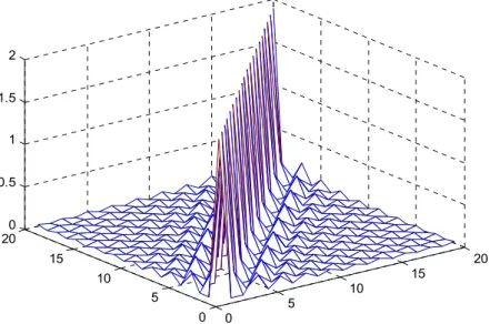
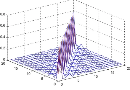
In past literatures, the second term associated with HB is treated as the interference part

due to MCFOs and should be avoided. However, we observe that when MCFOs increase H_B

becomes too large to be treated as interference. Instead, it is better to consider HB as a part

of signal too. The following diagrams show that the magnitude of HA and HB wax and wane

in different MCFOs condition.

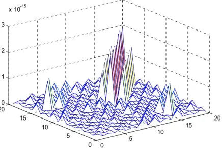
0 5 10 15 20 0 5 10 15 200 0.5 1 1.5

Fig. 3.2 A magnitude of the channel HA when |εR₁−εR₂ | 0=

0 5 10 15 20 0 5 10 15 200 1 2 3 x 10-15

(21)

0 5 10 15 20 0 5 10 15 200 0.5 1 1.5 2

Fig. 3.4 A magnitude of the channel HA when |εR₁−εR₂| 0.4=

0 5 10 15 20 0 5 10 15 200 0.2 0.4 0.6 0.8

(22)

0 5 10 15 20 0 5 10 15 200 0.2 0.4 0.6 0.8

Fig. 3.6 A magnitude of the channel HA when |εR1−εR2| 0.8=

0 5 10 15 20 0 5 10 15 200 0.2 0.4 0.6 0.8

(23)

3.1.3 Detection

With increase of the MCFOs, both H1 and H2 deviate from a diagonal matrix, but the

major power accumulate closely around the diagonal. The Minimum Euclidean distance decision is used consequently, and it can be expressed as

(1) (2) * ˆ _{arg min} i k k k i k i X r h h ζ ζ ζ = − − (3.9), where ζ denotes constellation point for M-ary modulation, i=1, …, M, k is the i

subcarrier index.

3.2 Iterative ICI Feedback Cancellation

This part introduces iterative ICI cancellation. Consider a parallel interference cancellation (PIC) scheme at each sub-carrier for data detection to reduce the error floor caused by multiple CFOs. Iterative interference cancellation is usually used to combat the multiple access interference (MAI). In OFDM systems, time variations are known to corrupt the orthogonality of the OFDM subcarrier. In this case, like MAI, ICI occurs because signal components from one subcarrier spill into other. That is

1 2 1 1 ( ) ( 1) ( 1) , 1, 1, , 2, 2, 0 0 0 ˆ ˆ ₀ R R k N N r r r k k k m R m R m k m R m R m m m m k m k Y r Y _Y − _{G H}ε _X − − _{G H}ε _X − _r = = ≠ ≠ = ⎧ ⎪ = ⎨ − − > ⎪ ⎩

∑

(3.10), where ( ) 1 ˆ r R X _and ( ) 2 ˆ r R

X _{represent for the symbol decisions of the r-th iteration. The}

decisions with interferences are used as the initial values. As the iteration number increases, more precise estimates of the transmitted symbols can be obtained.

(24)

3.3 Simulation Results

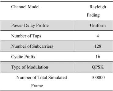
In this section, we present some simulation results to illustrate the performance of the proposed MCFOs compensation algorithm. The SFBC-OFDM system uses Alamouti’s scheme with two distributed relay nodes. The simulation assumes perfect channel state information (CSI) known and perfect CFOs known at destination node. The simulation parameters are listed in TABLE 3.2.

Fig. 3.8 depicts the BER performance whenεR₁ =0.4, 0.4εR₂ = − , i.e., related CFO = 0.8

when no channel coding is applied. It shows that the performance is poor without iterative parallel interference cancellation (PIC). With PIC, the performance is improved. It is also shown that proposed scheme can further improve the BER performance when compared with [9].

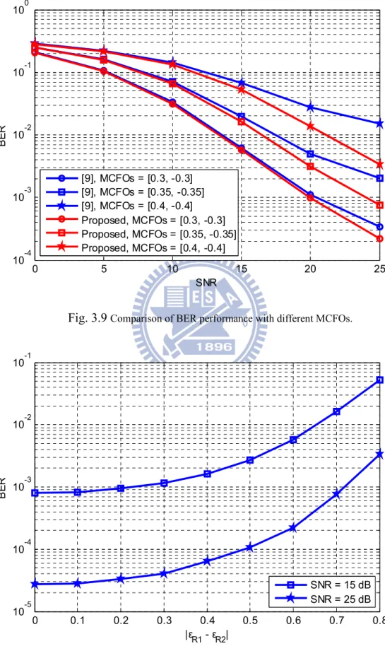
Fig. 3.9 compares the BER performance with different MCFOs. PIC with 5th iteration is applied in both cases. We find that when the relative CFO is larger, the performance is better than that of [9]. The phenomenon can be explained as follows. At low SNR, AWGN is dominant over ICI terms, so BER decrease with the increase of SNR. However, when SNR increases, ICI terms will be dominant over AWGN. Along the way, the ICI terms become larger as relative CFO increases. Therefore, it can be predicted to further improve the BER performance. Moreover, The Alamouti diversity can be maintained up to when relative CFO is 0.8. The tolerance range increases to relative CFO is 0.7.

Fig. 3.10 shows the BER performance versus the relative CFO with SNR = 15 and 25 dB. This shows the tolerance to MCFOs by deploying our proposed scheme.

(25)

TABLE 3.2 Simulation Parameter

Channel Model Rayleigh

Fading Power Delay Profile Uniform

Number of Taps 4

Number of Subcarriers 128

Cyclic Prefix 16

Type of Modulation QPSK

Number of Total Simulated Frame 100000 0 5 10 15 20 25 10-3 10-2 10-1 100 SNR BE R [9] [9] (1th iteration) [9] (5th iteration) Proposed Proposed (1th iteration) Proposed (5th iteration)

(26)

0 5 10 15 20 25 10-4 10-3 10-2 10-1 100 SNR BE R [9], MCFOs = [0.3, -0.3] [9], MCFOs = [0.35, -0.35] [9], MCFOs = [0.4, -0.4] Proposed, MCFOs = [0.3, -0.3] Proposed, MCFOs = [0.35, -0.35] Proposed, MCFOs = [0.4, -0.4]

Fig. 3.9 Comparison of BER performance with different MCFOs.

0 0.1 0.2 0.3 0.4 0.5 0.6 0.7 0.8 10-5 10-4 10-3 10-2 10-1 |ε_R1 - ε_R2| BE R SNR = 15 dB SNR = 25 dB

(27)

Chapter 4 Maximum Likelihood Sequence

Estimation for Alamouti Decoding

In chapter 3, we use Parallel Interference Cancellation (PIC) to further improve BER performance but encounter a latency issue. Therefore, we try to find other solutions which do not require iterations and maintain good performance. Consequently, we study [20] in which the OFDM signal is detected in doubly selective channels via an MLSE after whitening the residual intercarrier interference (ICI) plus noise. The step is to first get the covariance matrix of the noise plus residual ICI which is caused by Doppler affect. And the covariance matrix remains almost constant any changing parameters, such as Doppler frequency, SNR, the size of FFT and so on. Then a fixed whitening filter is devised to whiten the residual ICI plus noise, and an MLSE detector follows to decode the signal. In this chapter, we try to follow the approach and apply it to the MCFOs case.

(28)

4.1 Whitening By Inversion of the Covariance Matrix

Now, we rewrite Eq.(3.8) into follows

1 2, 2, * 2 * * 1,d 1,offd d offd * * 1,d 2,d 1,offd 2,offd * 1,d 2,d r = H X + H X + N = H X + H X + H X + H X + N = H X + H X + (H X + H X + N) = H X + H X + Z (4.1), where * * * * * * * * * * * * * * * * * * * * * * * * ⎡ ⎤ ⎢ ⎥ ⎢ ⎥ ⎢ ⎥ ⎢ ⎥ ⎢ ⎥ = ⎢ ⎥ ⎢ ⎥ ⎢ ⎥ ⎢ ⎥ ⎢ ⎥ ⎢ ⎥ ⎣ ⎦ d H * * * * * * * * * * * * * * * * * * * * * * * * * * * * * * * * * * * * * * * * ⎡ ⎤ ⎢ ⎥ ⎢ ⎥ ⎢ ⎥ ⎢ ⎥ ⎢ ⎥ = ⎢ ⎥ ⎢ ⎥ ⎢ ⎥ ⎢ ⎥ ⎢ ⎥ ⎢ ⎥ ⎣ ⎦ offd H

H2,d has the same matrix form which likes H1,d , H2,offd also has the same matrix form which

likes H1,offd. This means we handle 2p terms of nearest- neighbor ICI as signal and the outside

terms is the residual ICI. r is the sequence with colored noise Z and Rw is the covariance

matrix of Z. The inversion of the covariance matrix is based on eigenvalue decomposition. Eq. (4.1) is then transformed into

{ { 1 2 − -1 -1 -1 2 2 2 w 1,w 2,w * W W 1,d W 2,d W Z r H H * 1,w 2,w w R r = R H X + R H X + R Z r = H X + H X + Z $ 14243 14243 $

(4.2),

(29)

where 1 2

− -1

2 H W

R = UD U , U is the orthonormal eigenvectors matrix and D is the eigenvalues matrix.

4.2 MLSE Equalizer based on Viterbi Algorithm

MLSE is one of the most effective techniques for equalization [18]. A MLSE equalizer

determines a sequence s as the most likely transmitted sequence when the condition

probabilityP

( )

y s is maximized. Therefore, the maximization of the conditional probability | is equivalent to minimization operation of the Euclidean distance [19] and here it can be written as follows

=arg min || − ||2

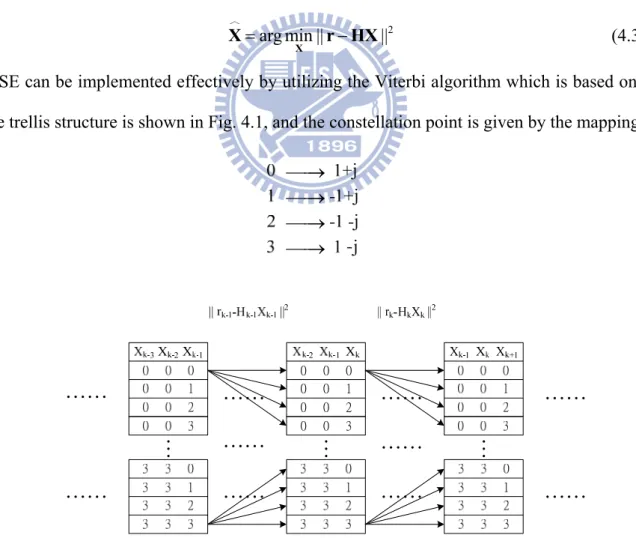
X

X＾ r HX (4.3), MLSE can be implemented effectively by utilizing the Viterbi algorithm which is based on a state trellis structure is shown in Fig. 4.1, and the constellation point is given by the mapping

⎯⎯→ ⎯⎯→ ⎯⎯→ ⎯⎯→

M

(30)

4.3 Simulation Results

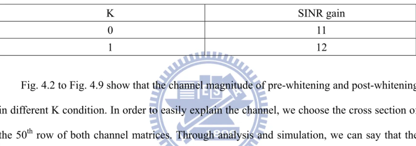
As in literature [20]. We choose K= 0, 1. The signal to interference plus noise ratio (SINR) gain within different K is showed in TABLE 4.1.

of pre-whitenig gain of post-whitenig SINR SINR SINR =

TABLE 4.1 SINR gain in different K value in SD case

K SINR gain

0 11 1 12 Fig. 4.2 to Fig. 4.9 show that the channel magnitude of pre-whitening and post-whitening

in different K condition. In order to easily explain the channel, we choose the cross section of

the 50th row of both channel matrices. Through analysis and simulation, we can say that the

SINR gain increase after whitening, but we need to increase the range to do MLSE in our case. It would cause the complexity to high so that the implementation is a question.

(31)

0 20 40 60 80 100 120 140 0 0.2 0.4 0.6 0.8 1 1.2 1.4

Fig. 4.2 The magnitude of 50th_{row of H}

1 when K = 0 0 20 40 60 80 100 120 140 0 0.5 1 1.5 2 2.5 3

(32)

0 20 40 60 80 100 120 140 0 0.1 0.2 0.3 0.4 0.5 0.6 0.7 0.8 0.9

2 when K = 0 0 20 40 60 80 100 120 140 0 0.1 0.2 0.3 0.4 0.5 0.6 0.7

2,w when K = 0

(33)

0 20 40 60 80 100 120 140 0 0.1 0.2 0.3 0.4 0.5 0.6 0.7

1 when K =1 0 20 40 60 80 100 120 140 0 0.2 0.4 0.6 0.8 1 1.2 1.4

(34)

0 20 40 60 80 100 120 140 0 0.05 0.1 0.15 0.2 0.25

2 when K = 1 0 20 40 60 80 100 120 140 0 0.05 0.1 0.15 0.2 0.25 0.3 0.35

(35)

Chapter 5 MLSE for Spatial Multiplexing

5.1 Spatial Multiplexing in Cooperative Communication

In this chapter, we try to apply the approach in [20] to the case of spatial multiplexing (SM). The cooperative communication system model with one source node, two relay nodes, and one destination node with two antennas is shown in Fig.5.1.

1

Y

2

Y

(36)

The mathematical derivation is = + + = + + R1 R2 R1 R2 ε ε 1 11 R1 12 R2 1 ε ε 2 21 R1 22 R2 2 Y G H X G H X W Y G H X G H X W (5.1), ⎡ ⎤ ⎡ ⎤ ⎡ ⎤ ⎡ ⎤ =_⎢ _⎥ + ⎢ ⎥ ⎢ ⎥ ⎢ ⎥ ⎣ ⎦ ⎣ ⎦⎣ ⎦ ⎣ ⎦ R1 R2 R1 R2 ε ε 1 11 12 R1 1 ε ε 2 21 22 R2 2 Y G H G H X W Y G H G H X W

(5.2),

where G and εR1 G is the ICI coefficient, εR2

[

]

0 2 4 X X X = R1 X _{L ,}

[

X1 X3 X5

]

= R2

X _{L . Finally, it can be written as follows}

Y = HX + W

(5.3),

where X=

[

X₁ X₂ X₃ _{L .}

]

5.2 Simulation Results

First of all, Fig. 5.2 to Fig. 5.4 shows that the channel matrix of SM in different MCFOs condition. When the MCFOs become large, the channel magnitude would not concentrate around the diagonal anymore. Unfortunately, this phenomenon caused by MCFOs is quite different from what have been observed in the case of Doppler affect.

If we still want to use this method of [20], we have to choose the MCFOs value which is not too large. Because the MCFOs value is not too large, the channel magnitude will concentrate around the diagonal. We choose MCFOs value that are within 0.4 and K= 0, 1. Finally, we calculate the signal to interference plus noise ratio (SINR) gain with different K is showed in TABLE 5.1. When K = 0, the SINR gain is only 1.04. This means that whitening or

(37)

not will not greatly affect the performance. Therefore, we choose the condition of K = 1 to further the investigation. Moreover, the normalized correlation at K = 1 shows in Fig. 5.5. The figure shows that the covariance matrix will not remain approximately constant as it does in the case studied in [20].

Fig. 5.6 and Fig. 5.7 show that the channel magnitude of pre-whitening and post-whitening. In order to easily explain the channel, we choose the cross section of the 50th row of both channel matrices. Fig. 5.7 shows that we have to include at least four off diagonal terms to get the performance improvement. Therefore, the calculative complexity is a problem. of pre-whitenig gain of post-whitenig SINR SINR SINR =

TABLE 5.1 SINR gain in different K value in SM case

K SINR gain

0 1.04 1 1.5

(38)

20 40 60 80 100 120 20 40 60 80 100 120

Fig.5.2 The channel matrix of SM when |εR₁−εR₂ | 0= .

20 40 60 80 100 120 20 40 60 80 100 120

(39)

20 40 60 80 100 120 20 40 60 80 100 120

Fig.5.4 The channel matrix of SM when |εR₁−εR₂ | 2= .

0.1 0.2 0.3 0.4 0.5 0.6 0.7 0.8 0 0.1 0.2 0.3 0.4 0.5 0.6 0.7 0.8 0.9 1 |ε_R1 - ε_R2| nor m al iz ed c or rel at io n r=2 r=4

(40)

0 20 40 60 80 100 120 140 0 0.05 0.1 0.15 0.2 0.25 0.3 0.35 0.4 0.45 0.5

Fig. 5.6 The magnitude of 50th_{row of H at K = 1}

0 20 40 60 80 100 120 140 0 0.2 0.4 0.6 0.8 1 1.2 1.4

(41)

Chapter 6 Summary

6.1 Conclusions

Various compensation schemes of synchronization errors in the cooperative MIMO system are investigated in this thesis. We used a modified SFBC decoding and detection rule to improve the performance. Iterative interference cancellation is used to further mitigate the ICI and reduce the error floor. Through simulation results it has been show that the BER performance and tolerance range of MCFOs is superior. The Alamouti diversity can be maintained up to when relative CFO is 0.8.

We also investigate other ways to improve the performance, especially the approach of using MLSE with whitening proposed in [20]. We apply this method to both the cases of spatial diversity and spatial multiplexing. However, simulation and analysis show that this approach may not be suitable for combating MCFOs.

6.2 Future Work

(42)

Bibliography

[1] K. F. Lee and D. B. Williams, “A space-frequency transmitter diversity technique for

OFDM systems,” IEEE GLOCOM., vol. 3 pp. 1473-1477, Nov. 2000.

[2] A. Sendonaris, E. Erkip and B. Aazhang, “User cooperative diversity part I: system

description; part II: implementation aspects and performance analysis,” IEEE Trans.

Commun., vol. 51, pp. 1927-1948, Nov. 2003.

[3] F. Tian, X.-G. Xia, and P. C. Ching, “Equalization in space-frequency coded cooperative

communication system with multiple frequency offsets,” IEEE ISSCS, vol. 2, pp. 1-4,

July. 2007.

[4] H. Wang, X.-G. Xia, and Q. Yin, “Distributed space-frequency codes for cooperative

communication systems with multiple carrier frequency offsets,” IEEE Trans. Wireless

Commun., vol. 8, pp. 1045-1055, Feb. 2009.

[5] Q. Huang, M. Ghogho, and J. Wei, “Data detection in cooperative STBC-OFDM systems

with multiple frequency offsets,” IEEE Signal Proc. Letters, vol. 16, pp. 600-603, July.

2009.

[6] Z. Li and X.-G. Xia, “An Alamouti coded OFDM transmission for cooperative systems

robust to both timing errors and frequency offsets,” IEEE Trans. Wireless Commun., vol.

7, no. 5, pp. 1839-1844, May. 2008.

[7] Y. Zhang, “Multiple CFOs compensation and BER analysis for co-operative

communication systems,” in Proc. IEEE WCNC’09, pp. 1-6, Apr. 2009.

[8] D. Sreedhar and A. Chockalingam, “ICI-ISI mitigation in cooperative SFBC-OFDM with carrier frequency offset,” in Proc. IEEE PIMRC’07, pp. 1-5, Sept. 2007.

(43)

[9] Tsung-Ta Lu, Hsin-De Lin, and Tzu-Hsien Sang, "An SFBC-OFDM Receiver to Combat

Multiple Carrier Frequency Offsets in Cooperative Communications" IEEE PIMRC

2010.

[10] T. D. Nguyen, O. Berder, and O. Sentieys, “Efficient space time combination technique

for unsynchronized cooperative MISO trans-mission,” IEEE VETECS’08, pp. 629-633,

May. 2008.

[11] Y. Mei, Y. Hua, A. Swami, and B. Daneshrad, “Combating synchron-ization errors in

cooperative relays,” in Proc. IEEE ICASSP’05, vol. 3, pp. 369-372, Philadelphia, Pa,

USA, Mar. 2005.

[12] J. N. Laneman and W. Wornell, “Distributed space-time-coded pro-tocols for exploiting

cooperative diversity in wireless networks,” IEEE Trans. Inform. Theory, vol. 49, pp.

2415-2425, Oct. 2003.

[13] Y. Jing and B. Hassibi, “Distibuted space-time coding in wireless relay networks,” IEEE

Trans. Wireless Commun., vol.5, pp. 3524-3536, Dec. 2006.

[14] A. Yilmaz, “Cooperative diversity in carrier frequency offset,” IEEE Commun. Letters,

vol. 11, pp. 307-309, Apr. 2007.

[15] W. Zhang, D. Qu, and G. Zhu, “Performance investigation of distribu-ted STBC-OFDM

system with multiple carrier frequency offsets,” in Proc. IEEE PIMRC’06, pp. 1-5, Sept.

2006.

[16] D. Veronesi and D. L. Goeckel, “Multiple frequency offset compen-sation in cooperative

wireless systems,” in Proc. IEEE GLOCOM., pp. 1-5, Nov. 2006.

[17] P. H. Moose, “A technique for orthogonal frequency division multi-plexing frequency

offset correction,” IEEE Trans. Commun., vol. 42, no. 10, pp. 2908-2914, Oct. 1994.

[18] G. D. Forney, “Maximum-likelihood sequence estimation of digital sequences in the

presence of intersymbol interference”, IEEE Trans. Commun., vol. 18, no. 3, pp. 363-378,

(44)

[19] J. G. Proakis and M. Salehi, Digital Communications, 5th ed. New York: McGraw-Hill,

2008.

[20] Hai-wei Wang, Lin, D.W., Tzu-Hsien Sang, “OFDM Signal Detection in Doubly

Selective Channels with Whitening of Residual Intercarrier Interference and Noise,”

(45)

About the Author

姓名：李俊育 Jyun-Yu Lee

出生地：台灣省彰化縣

出生日期：1984. 09. 13

學歷：1991. 09 ~ 1997. 06

彰化縣溪湖國民小學

學歷：1997. 09 ~ 2000. 06

彰化縣溪湖國民中學

學歷：2000. 09 ~ 2003. 06

彰化縣彰化高級中學

學歷：2003. 09 ~ 2008. 06

中原大學電機工程學系學士

學歷：2008. 09 ~ 2011. 02

國立交通大學電子研究所系統組

碩士

合作式通訊下以多輸入多輸出和正交分頻多工之接收端對抗多重頻率偏移

國立交通大學

電子工程學系 電子研究所碩士班

碩

士 論 文