隨機光柵化在裁切空間下採樣點剔除技術

全文

(1)國立交通大學多媒體工程研究所碩士論文. 隨機光柵化在裁切空間下採樣點剔除技術 Clip Space Sample Culling for Stochastic Rasterization. 研究生：吳怡正指導教授：施仁忠. 中華民國. 教授. 一百零二. 年七月.

(2) 隨機光柵化在裁切空間下採樣點剔除技術 Clip Space Sample Culling for Stochastic Rasterization. 研究生：吳怡正. Student：Yi-Jeng Wu. 指導教授：施仁忠. Advisor：Prof. Zen-Chung Shih. 國立交通大學多媒體工程研究所碩士論文. A Thesis Submitted to Institute of Multimedia Engineering College of Computer Science National Chiao Tung University in partial Fulfillment of the Requirements for the Degree of Master in. Multimedia Engineering July 2013 Hsinchu, Taiwan, Republic of China. 中華民國一百零二年七月.

(3) 隨機光柵化在裁切空間下採樣點剔除技術. 研究生: 吳怡正. 指導教授: 施仁忠教授. 國立交通大學多媒體工程研究所. 摘要. 在渲染真實的相機影像時，兩種現象是很常見的：動態模糊(motion blur)與景深模糊(defocus blur)。我們提出了一個針對動態與景深模糊在隨機光柵化技術下的裁切空間(clip-space)採樣點剔除技術。這個二階段的測試利用裁切空間下的資訊去降低我們需要做的覆蓋測試採樣點數量，包含鏡頭座標與時間座標下的所有採樣點。首先我們做一個簡略的測試取得保守的鏡頭座標範圍值，並去除在此範圍之外的採樣點。在第二階段的測試時我們在裁切空間下針對每個三角形頂點找出 xyuvt 空間的相似三角形的關係，藉由此三角方程式去剔除不屬於此範圍內的採樣點。本篇論文提供了在即時運算的隨機光柵化中的簡單採樣點剔除方法，並且在少量的運算下可達到良好的採樣點測試效率(sample test efficiency)。. I.

(4) Clip Space Sample Culling for Stochastic Rasterization Student: Yi-Jeng Wu. Advisor: Prof. Zen-Chung Shih. Institute of Multimedia Engineering National Chiao-Tung University. Abstract. To render realistic camera images, two effects are common : motion blur and defocus blur. We present a novel clip space culling test of stochastic rasterization of motion and defocus blur. This 2-stage test use the clip space information to reduce the samples needed to be coverage tested over camera lens domain (uv) and time domain (t). First we do a rough test to get a conservative range of the camera lens uv bound, and cull the samples outside this bound. Then the second test finds a similar triangular equation for each triangle vertex in xyuvt space. Based on this equation, we cull the rest of samples outside. We present a simple method for the real-time stochastic rasterizer, and achieve a good sample test efficiency with low computation cost.. II.

(5) Acknowledgements. First of all, I would like to express my sincere gratitude to my advisor, Pro. Zen-Chung Shih for his guidance and patience. Without his encouragement, I would not complete this thesis. Thanks also to all the members in Computer Graphics and Virtual Reality Laboratory for their reinforcement and suggestion. Thanks for those people who have supported me during these days. Finally, I want to dedicate the achievement of this work to my family.. III.

(6) Contents ABSTRACT (in Chinese)…………………………………………………………….I ABSTRACT (in English)………………………………………………………….II ACKNOWLEDGMENTS………………………………………………………….III CONTENTS………………………………………………………………………IV LIST OF FIGURES………………………………………………………………….V LIST OF TABLES…………………………………………………………………VI CHAPTER 1 Introduction…………………………………………………………1 1.1 1.2 1.3. Motivation………………………………………………………………………..1 System Overview………………………………………………………………...2 Thesis Organization…………………………………………………………….3. CHAPTER 2. Related Works………………………………………………………5. CHAPTER 3 Algorithm………………………………………………. . …………8 3.1 3.2 3.3 3.4 3.5. Stochastic Rasterization……………………………………………………….9 Bounding the Moving/Defocus Range………………………………………10 Culling Stage 1………………………………………………………………….12 Culling Stage 2………………………………………………………………….14 Controllable Defocus Blur…………………………………………………… 18. CHAPTER 4. Implementation and Results……………………………………20. CHAPTER 5. Conclusion and Future Work…………………………………….31. REFERENCE……………………………………………………………………..32. IV.

(7) List of Figures Figure 1.1: System overview. …………………………………………………………4 Figure 3.1: Create 2D bounding box ………………………………………………11 Figure 3.2: Crossing z=0 plane ……………………………………………………11 Figure 3.3: 2D convex hull …………………………………………………………12 Figure 3.4: A ray is shot from camera to screen pixel and intersects with the focus point … …………………………………………………………………13 Figure 3.5: Ray intersection with moving vertex ……………………………………14 Figure 3.6: Ray intersection with two similar triangles……………………………15 Figure 3.7: The rational function is bounded by two liear bounds…………………17 Figure 3.8: Combine of all 3 pairs of linear bounds with 2 linear bounds(Red lines) ……………………………………………………………………17 Figure 4.1: The rational function is bounded by two liear bounds…………………22 Figure 4.2: Defocus blur with different focus depths………………………………24 Figure 4.3: Racing car with/without motion blur……………………………………25 Figure 4.4: Flying Dragonfly with/without camera motion blur……………………26 Figure 4.5: FairyForest with/without both motion and defocus blur………………27 Figure 4.6: Difference between enlarge focus range our not………………………28. V.

(8) List of Tables Table 4.1: STE results with 16spp. Higher is better…………………………………29 Table 4.2: Computation time results with 16spp. Lower is better .………………….30. VI.

(9) Chapter 1 Introduction 1.1 Motivation Traditional rasterization is based on two assumptions, the pinhole camera and extremely fast shutter. These two assumptions will lead to some differences between the image we rendered and the image in real world, such as motion blur and defocus blur. Motion blur is caused by non-zero shutter time, objects moved during shutter time causing motion blur on the image. Defocus blur is caused by camera lens. Object not on focus depth goes through different camera lens positions will be formed at different image locations.. Motion blur can resolve temporal aliasing problems, and defocus blur can control user’s attention on the image. To achieve real-time rendering, point sampling is a good way. In stochastic rasterization. We average these sample colors as pixel color. These samples have 5 dimensions. Besides traditional (x,y) coordinates, there is also time dimension (t) and camera lens dimensions (u,v).. In traditional rasterizer, we build a 2D bounding box on the screen for the triangle. Then we test all samples inside this bounding box. But most of these samples are not visible. For example, a moving triangle only passes a pixel at time dimension 1.

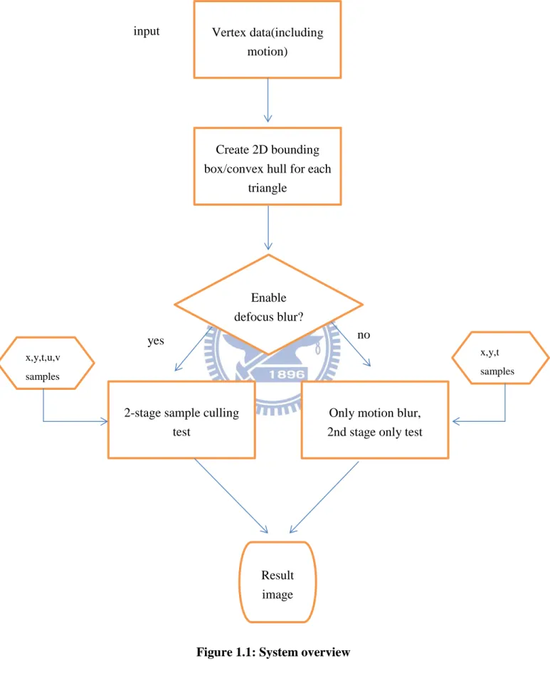
(10) close to 0.3. Then all stochastic samples far from this time will not be visible. That is, most of the sample tests failed. The stochastic rasterizer’s performance has a predictor: sample test efficiency (STE), which is the percentage of valid coverage samples in all test samples [4]. A good visibility test gets higher STE. Our objective is to design a sample visibility test not being dependent on the amount of motion and defocus blur. Use this algorithm to cull non-visible samples and reach high STE.. Our contributions are as follows: 1. We design a two-stage sample culling algorithm for both motion and defocus blurred stochastic rasterization with low-cost computing. 2. High STE is achieved. 3. The algorithm can handle not only just motion blur or defocus blur, but also both effects simultaneously.. 1.2 System Overview Our system renders the camera-like images by the following steps: 1. Generate 2D bounding box/convex hull for each triangle in geometry shader. 2. Test the stochastic samples inside these bounding boxes roughly in stage 1. 3. Test the rest samples in stage two, only samples that pass all tests will do the actual triangle interception/coverage test indeed. Figure 1.1 shows the flow of our proposed system.. In our culling algorithm one, we do the rough camera lens test. Find out the moving triangle’s maximum and minimum camera lens range. Then cull all samples outside this range [umax , umin] , [vmax , vmin]. 2.

(11) Then we will apply an accurate test. We use a triangular equation-like relationship in clip space. By using this information, we can cull samples with both time dimension (t) and camera lens dimension (u,v). For each pixel , we only need to compute this equation once. Then every different sample dimensions can use the same test for culling.. Finally, the system will test the remaining samples and render the final image. We can render motion blurred only or defocus blurred only image, or both effects at the same time.. 1.3 Thesis Organization The rest of the thesis is structured as follows: Chapter 2 reviews the related works of stochastic rasterizations on motion and defocus blur. Chapter 3 describes our two-stage culling algorithm of stochastic rasterization. Chapter 4 describes our implementation detail, results and system performance. Finally, we conclude this research with limitation and future work in Chapter 5.. 3.

(12) input. Vertex data(including motion). Create 2D bounding box/convex hull for each triangle. Enable defocus blur? no. yes x,y,t,u,v. x,y,t. samples. samples. 2-stage sample culling test. Only motion blur, 2nd stage only test. Result image. Figure 1.1: System overview. 4.

(13) Chapter 2 Related Works In this chapter, we review related previous works. Existing blurry effects rendering often use post processing. We will not discuss these methods. First we focus on traditional sampling methods with the 5D space of pixel location (x,y), time t and lens position (u,v). Then we briefly survey the technique of stochastic rasterization that reduce the computation cost for blurry rendering.. Haeberli and Akeley [7] proposed a hard ware supported method called accumulation buffer. It renders multiple images in each buffer. Then average pixel values as the final color. If we render enough number of images, this brute-force method will get a good result. But the computation cost is very high. If the number of rendered images is reduced, the “ghosting” artifact could appear.. Stochastic rasterization renders image once with multiple samplings. Each sample has a unique sampling dimensions (x,y,t,u,v).. Fatahalian et al. [4] presented the InterleaveUVT algorithm. They use as many samples as possible in accumulation buffer. For example: 4 images = 4 samples per pixel. But these samples come from different time steps and lens locations. For example, if we have 16 images at different time steps, we use only 4 of them. Each 5.

(14) pixel use different 4 images. This is an enhancement of accumulation buffer. But there is still a discrete set of individual u, v, t values can be used. This will cause the banding artifact.. Akenine-Möller et al. [1] create a bounding box for each moving triangle on screen space. Then they test all stochastic samples inside this bounding box. McGuire et al. [13] escalate this oriented bounding box into 2D convex hull, which makes the testing area smaller. However, most of the samples inside these bounding boxes/2D convex hulls do not hit the triangle. In fact, if we look at a pixel which is inside the triangle at time = 0, it seems impossible that the samples with high t values could be covered if the motion is large. To make the sample test more efficient, solving the sample visibility problem is a major challenge. That is, if we can reject samples that can’t be hit, the sample test efficiency (STE) would increase.. Laine et al. [10] use a dual-space culling algorithm to solve the visibility test. For the defocus blur, they use the linear relation ship between the lens location and the space location. By interpolating two axis aligned bounding boxes of the triangle on lens locations (0,0) and (1,1), they can get the maximum and minimum lens location on the pixel. With the motion blur, the world space affine motion is not affine in screen space. For example, an object moves from far to near linearly. It will move faster and faster in screen space. So we cannot use simple interpolation to find the relative time dimension bounds. They create a dual-space to convert the equation in clip space by -. 6.

(15) where γ is the viewing direction. In this equation, δ is linear with. and ω. Besides. and ω are both linear with time t. So we can say δ is linear with t. They use this linear relationship to get the time bounds by linear interpolation. Munkberg et al. [15] propose a hyper plane culling algorithm. They use the equation between object location, lens coordinate, and time coordinate to find linear bounds in ut- and vt-space. They also create a hyper plane in xyuvt-space for each triangle edge to cull samples. This hyper plane culling algorithm is selectively enabled while the blurry area is large enough. Our method use the similar idea to create linear bounds in clip space using the triangle similarity relationship. By using these bounds to reduce the number of sample tests, we can obtain better performance.. 7.

(16) Chapter 3 Algorithm In this paper, we introduce a novel 2-stage sample culling test for stochastic rasterization of motion and defocus blur. We assume that the motion of triangles is linear in world space in shutter times. The steps of our algorithm work as follows for each triangle. Each pixel is sampled at different 5D sample locations (x,y,t,u,v). Note that all steps take place on shaders.. 1. For each triangle, create a corresponding’s bound geometry 2D convex hull (if motion blur only) or bounding box in screen space. 2. For each pixel inside the box, test the stochastic 5D-dimension samples. 3. For each sample, apply the 1st stage culling test and cull the sample outside the rough camera lens bounds. 4. If the sample passes the stage 1 test, apply the 2nd stage test. This test uses the triangle equation in clip space with point’s information. Find out the time bounds of each (u,v) location samples. 5. Only samples pass both 1st and 2nd stages need a complete triangle intersection test.. The rest of this chapter is organized as follows. In Section 3.1, we show how to render motion blur and defocus blur images with stochastic rasterizer. In Section 3.2, we describe the initial 2D convex hull/bounding box. In Section 3.3, we describe the 8.

(17) 1st stage culling test and Section 3.4 for the 2nd stage test. Finally in Section 3.5, we describe an application to control the defocus blur range by Munkberg et al. [17].. 3.1 Stochastic Rasterization To render motion blurred images, we need to input triangles at time t = 0 and t = 1. That is, the triangle positions when shutter opens and closes. Then, for each pixel covered the moving triangle, we test different stochastic samples at different time coordinate. Similar to the ray intersection test. We shoot a ray from a pixel and test if the ray intersects with triangle at time t. If the intersection happens, we add the color value of the intersection point. Otherwise we discard this sample. Finally we average valid sample colors as the pixel color.. To render defocus blurred image, we need the lens radius to compute the circle of confusion (CoC). We use a simple physically-based CoC setting. It is linearly dependent on the depth w in clip space, i.e., CoC(w) = a+wb . Parameters a and b are constant derived from the camera’s aperture size and focal distance. The out of focus vertex position is changed to different camera lens coordinates. That is, a vertex position (x,y,z) in clip space. If we use camera lens (u,v) to see this vertex, it’s position will change into (x + uc , y + vc , z), where c = a + zb. For a pixel, only a position in lens coordinates can see this vertex. The intersection test is similar to the previous one. The ray checks the intersection test with the triangle in lens coordinates.. For the case of both effects exist, the intersection test should find out the triangle position in camera lens (u,v) and time coordinate (t). As we know, a lot of samples are not visible for a given pixel. Our goal is to increase the hit ration of sample test.. 9.

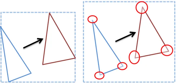
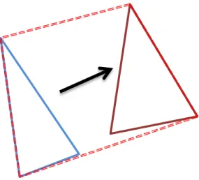
(18) 3.2 Bounding the Moving/Defocus Range For each triangle, we need to rasterize the bounding geometry large enough to cover the entire triangle’s motion. The most conservative bounding is the whole viewing frustum’s near plane. The tightest bounding geometry is the front-facing surfaces of the triangle’s swept volume, but this bound is curved on the sides. We use the 2D bounding box of the moving triangle at near plane to bound the motion triangle. If we rasterize in-focus images, we change the bounding box into convex hull.. To create the 2D bounding box, we need the vertex positions of triangles at the beginning and the end of the shutter time. The triangle transfers into screen space bounding box in geometry shader. First we project these 6 vertices into screen space and get the bounding box’s maximum and minimum boundary. Then we increase/decrease these boundaries, by passing the camera lens’s radius and the focus depth. We compute the maximum circle of confusion with the minimum and the maximum depth from the triangle vertices. Figure 3.1 shows how to create 2D bounding box. If the triangle passes the z = 0 plane, we find out the intersection point at the near plane from the 6 triangle edges and 3 moving point paths. Figure 3.2 shows this case.. If we render the in-focus image, only the motion blur effect is added. We make the bound tighter by using the 2D convex hull. We use Graham scan algorithm [Graham 1972] [5] to create this 2D convex hull. The reason why we don’t use this technique for defocus blur is that computing all these 6 circle of confusions with. 10.

(19) different depth taking too much cost, as shown in Figure 3.3.. (a) Without defocus. (b) With defocus (Red: circle of confusions) Figure 3.1: Create 2D bounding box. Z=0. Near. -z. +z. Figure 3.2: Crossing Z=0 plane. 11.

(20) Figure 3.3: 2D convex hull. 3.3 Culling Stage 1 Consider the vertex of a triangle in the clip space. We assume a linear motion, p(t) = (1-t)q + r, where q is the starting point and r is ending point. For defocus blur, in the signed clip space, we assume that the circle of confusion is linear with time, that is, c(t) = a + w(t)b. In stage 1 culling, the samples outside the camera lens bounds are culled.. The computation of these bounds is relatively simple because the clip-space vertex position is linear to lens coordinates. We normalize the lens by (u,v) ∈ [-1,1]2 . For each pixel covered by the triangle, we give stochastic samples with different parameters (t,u,v). Then we need to test if the triangle is visible from camera lens u and v in time t.. In Figure 3.4, a ray is shot from camera and passes through a screen pixel. We set this “screen pixel” as the focus point with our focus depth. In this xw space, we connect all 6 triangle vertices with the focus point. We will obtain 6 points at depth. 12.

(21) w=0. We take the maximum and minimum one as the camera lens bounds.. We can compute u = ( nx ⋅ p(t) ) / ( p(t).z – focusDepth ), where nx = ( -focusDepth , 0 , focusPoint.x) is the normal vector of the pixel ray. Then we divide this u by camera lens radius. Finally we get the normalized camera lens bounds at u dimension. The v dimension bound can be obtained in the same way with ny = ( 0 , -focusDepth , focusPoint.y).. w. t=1. t=0. W=focusDepth x. n. x umin. uMAX. Figure 3.4: A ray is shot from camera to screen pixel and intersects with the focus point. All 6 triangle vertices connect with this focus point and intersect with the camera lens at depth w=0. With these rough camera lens bounds, we cull the stochastic samples where u, v dimensions are outside the lens bounds. This makes higher STE further.. 13.

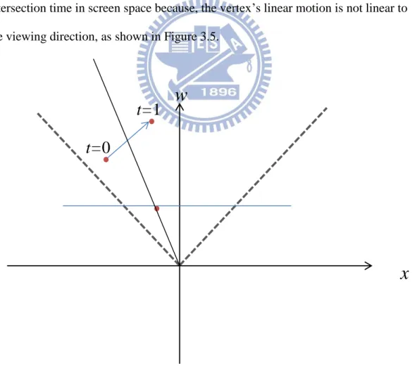
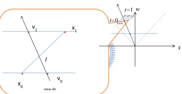
(22) 3.4 Culling Stage 2 After 1st stage culling, samples outside camera lens bounds are culled. The remaining of samples would go into2nd stage test. We test the samples with each u, v dimensions and find out the corresponding time bounds.. Consider the triangle vertices in clip space. The vertex will “translate” with different camera lens u, v relatively. For example, a vertex p = ( x , y , w ), we use camera lens ( u , v ) to see this vertex. It is translated into p’ = ( x + uc , y + vc , w ), where c is the circle of confusion of this vertex : c = a + wb. With shutter opened, we need to know when this pixel can see the triangle. It is hard to compute the intersection time in screen space because, the vertex’s linear motion is not linear to the viewing direction, as shown in Figure 3.5.. t=1. w. t=0. x. Figure 3.5 Ray intersection with moving vertex In order to obtain the intersection time, we find a triangle relationship in this clip. 14.

(23) space. First, for each sample, we compute two vertex positions with camera lens u, v at time t = 0 and t = 1, that is, x’(0) = x(0) + uc(0). ,. x’(1) = x(1) + uc(1).. The y coordinate can be obtained in the same way. Then we find the other 2 points with the ray shot from camera to pixel which intersects with the triangle vertex’s depth values when the shutter opened and closed.. t=1 w t=0. v1. x1 x I. x0. v0 view dir. Figure 3.6 Ray intersection with two similar triangles. Now we have 4 vertices in xw clip pace. Two points with camera lens u, v and their own circle of confusions c(t) when shutter opened and closed. The other 2 points are the viewing direction’s intersection points at the same depth value of the previous 2 vertices. Figure 3.6 shows all these four points. Then we can find two similar triangles, where their corresponding edges are proportional in length:. 15.

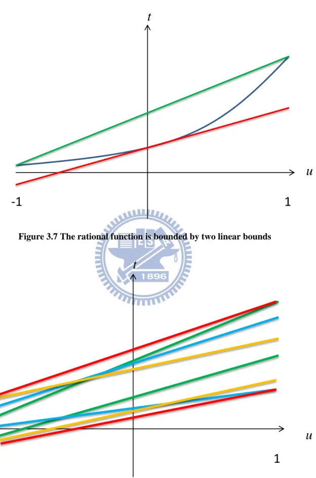
(24) Then the intersection time t can be obtained as follows: (1). We compute all 3 pair of triangle vertices at time t = 0 and t = 1 in xw and vw space. Then we get time bound [ tmax , tmin ]. All stochastic samples with t dimension outside this bound will be culled.. As we described before, we find the similar triangles in clip space. And use it to compute time dimension bounds. We have to compute each vertex position with stochastic sample’s u, v camera lens position. That is, for each sample, we have to compute the triangle vertex position p(0) = ( x + uc(0) , y + vc(0) , w). This takes too much cost.. By rewriting equation 1, each x can be replaced by x = x + u*c(t), we have : (. ). (. ). This is a rational function in u, and this function is also monotone, which can be bounded by two linear functions as shown in Figure 3.7.. 16.

(25) t. u -1. 1. Figure 3.7 The rational function is bounded by two linear bounds. t. u -. 1 Figure 3.8 Combine of all 3 pairs of linear bounds with 2 linear bounds (Red Lines). 17.

(26) The two linear bound are as follows: Green : ( ). (. Red : ( ). ( ). (. ). ( ). ). ( ( ) (. ). (. )) ( ). All 3 pairs of triangle vertices will create 2 linear bounds. We combine these linear bounds with 2 bounds, one is maximum bound [t(-1)MAX , t(1)MAX], and one minimum bound [t(-1)min, t(1)min]. By two linear bounds, we can test all stochastic samples at the same pixel (same viewing direction). If the time dimension is larger than upper bound or smaller than lower bound, the sample will be culled. That is, we only need to compute two linear bounds once for each pixel.. 3.5Controllable Defocus Blur People often want to control over depth of field parameters empirically, such as limit foreground blur or extend the in-focus range while preserving the foreground and background. MunKberg et al. [17] proposed a user controllable defocus blur method. We use their technique in our system.. We modify the circle of confusion by limited it’s size near the focus depth.. 0. ,. w-focusDepth < ε. C= a + wb ,. otherwise. 18.

(27) It is assumed that the clip space circle of confusion radius is linear in the interior of a triangle. Then we can increase the focus range or decrease the foreground blur easily. If the triangle vertex is inside the extended focus range, all samples pass stage 1 test. And set u = v = 0 to compute the stage 2 time bounds. Finally we modify the circle of confusion when doing the triangle intersection test and render the extended focus range blurry image.. 19.

(28) Chapter 4 Implementation and Results We develop our system based on openGL and GLSL. Our stochastic sample culling algorithm is implemented in pixel shader. In the CPU host, we bind the vertex stream and the transform matrix at shutter time t = 0. We also bind the texture coordinates and other shading attributes like vertex normal etc. as usual. We also bind the vertex at shutter time t = 1 as an additional vertex attribute.. Vertex Shader: We transform the vertices into clip space at shutter time t = 0 and t = 1. Then we pass all vertex attributes to the geometry shader.. Geometry Shader: In this shader, we convert each triangle into a 2D bounding box or a 2D convex hull as we described in Section 3.2. Since this method destroy the triangle’s structure, we should store the original all 6 vertices positions as output variables. Besides we pack each vertex’s circle of confusion and other vertex attributes from previous shader to every emitted vertex.. 20.

(29) Pixel Shader: In pixel shader, we deal with each pixel inside the 2D bounding box. The stochastic sample buffer is created in CPU host program, and passes into pixel shader as a texture. We create this buffer in 3 channels at time t and camera lens u, v. The time values are uniform in [0,1] as floating point. The camera lens value are uniform in [-1,1]. We set this buffer size as 128*128. Each pixel takes the stochastic samples from this texture.. We also use multi-sample antialiasing (MSAA) as well. For each pixel, we use a bit mask to store hit/miss of the samples. We use gl_SampleMask[] as the bit mask in openGL. Coverage for the current fragment will become the logical AND of the coverage. mask. and. the. output gl_SampleMask.. That. is,. setting. a. bit. in gl_SampleMask to zero will cause the corresponding sample to be considered uncovered for the purpose of multisample fragment operations. Finally we average the pixel values whose corresponding mask bit is equal to one. If the bit mask is all zero, we discard this pixel.. If the stochastic sample passes our culling test and the triangle intersection test, we draw the pixel color with the corresponding texture coordinate or the corresponding color. The GPU program flow is shown in Figure 4.1.. 21.

(30) Host program. Vertex stream. Vertex attributes Transform matrix Motion vector …. Pixel shader: Set vertex values. Triangles. CameraLensRadius CameraFocusDepth Nearplane …... Geometry shader: Transform triangle into 2D bounding box. 2D Bounding boxes Vertex positions CoCs. Viewportsize Diffuse texture Alpha texture Sample buffer ….. Pixel shader: Culling test Ray intersection test. Final color. Figure 4.1: GPU program workflow. 22.

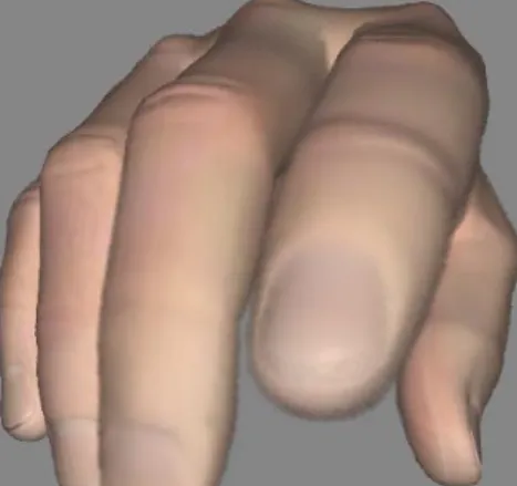
(31) In the remaining of this chapter, we present our result images rendered in real-time on a desktop PC with Intel Core i7 950 CPU 3.07GHz and NVIDIA GeForce GTX 580 video card. Our system is implemented in C++ Language using OpenGL and GLSL. All results are rendered with 1024 x 768 pixels.. For our stochastic rasterization culling algorithm, we compare two culling tests. Namely Liane et al.’s dual space [10] culling algorithm. And the traditional culling algorithm with bounding box. We test four different scenes. The scene Hand is tested with object’s motion blur (Figure 5.2). The FlyingDragonfly is tested with camera’s motion blur (Figure 5.3). The FairyForest is tested with both motion blur and defocus blur (Figure5.4). We also show the image with enlarge focus range (Figure 5.5). With increasing the focus range, the whole fairy face can be seen clearly. Note that all scenes are rendered by 32 samples per pixel.. 23.

(32) Figure 4.2: Defocus blur with different focus depths 24.

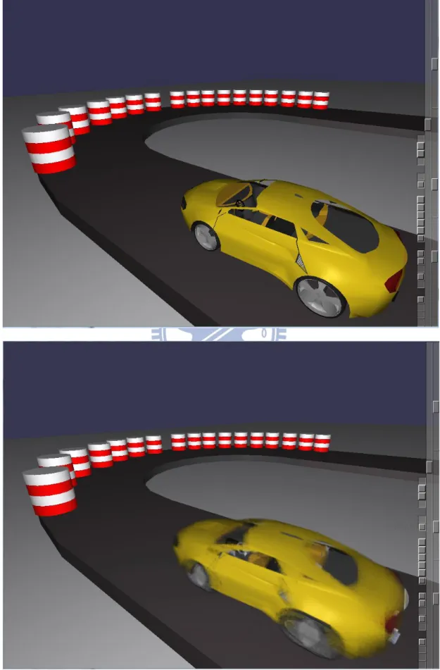
(33) Figure 4.3: RacingCar with/without motion blur 25.

(34) Figure 4.4: FlyingDragonfly with/without camera motion blur 26.

(35) Figure 4.5: FairyForest with/without both motion and defocus blur. 27.

(36) Figure 4.6: Difference between enlarge focus range or not. 28.

(37) Table 4.1 shows the result of STE. We compare our algorithm with the other two culling tests. The first scene Hand has 15k triangles, Car has 54k triangles ,Dragonfly and FairyForest has about 85k and 170k triangles. We can see that with motion blur or defocus blur only, our algorithm’s STE is almost the same as Dual space. Because our stages 1 and 2 culling algorithms are separately like the uv test and t test with Laine et al. [10]. But our algorithm comes better with both effects exist.. Scene. Bbox. Dual Space. Our. Hand Defocus blur. 12%. 29%. 29%. Defocus blur*2. 10%. 28%. 27%. Motion blur. 9%. 28%. 27%. Motion blur*2. 4%. 25%. 26%. Motion blur. 3%. 23%. 22%. Motion blur*2. 1%. 24%. 24%. Both blur. 0.4%. 5%. 19%. Both blur*2. 0.2%. 2%. 13%. Car. Dragonfly. FairyForest. Table 4.1: STE results with 16spp. Higher is better.. 29.

(38) Table 4.2 shows the computation time for each scene in millisecond. Our algorithm takes a little more computation time than Laine et al. [10] while rendering large motion scenes. But, we perform better when both effects exist.. Scene. Bbox. Dual Space. Our. Hand Defocus blur. 135 ms. 131 ms. 123 ms. Defocus blur*2. 140 ms. 133 ms. 126 ms. Motion blur. 178 ms. 156 ms. 158 ms. Motion blur*2. 185 ms. 172 ms. 166 ms. Motion blur. 156 ms. 140 ms. 136 ms. Motion blur*2. 161 ms. 148 ms. 138 ms. Both blur. 212 ms. 183 ms. 175 ms. Both blur*2. 222 ms. 202 ms. 188 ms. Car. Dragonfly. FairyForest. Table 4.2: Computation time results with 16spp. Lower is better.. 30.

(39) Chapter 5 Conclusions and Future Work In this thesis, we propose a 2-stage culling algorithm for stochastic rasterization. We propose a new idea to compute the time bounds with relative camera lens in clip space. Using these bounds to cull and get higher STE.. We cull samples outside camera lens bounds in stage1 using the linear relationship between camera lens and vertex position. Stage 2 culls samples outside time bounds. We use the triangle similarity in clip space to find the intersection time easily. We use this idea to compute two linear bounds. Each pixel only needs to compute these bounds once. Our algorithm can handle motion blur and defocus blur simultaneously.. In the future we would find some other improvement to find bounding geometry easily and more accurately. We shall try to reduce the execution time, such as increase the test range from per pixel test to per tile test. Furthermore we can make the STE higher with more “accurate” stochastic samples. We can use stage 1 result to generate relative stochastic samples with different camera lens. Then use stage2 result to set each previous sample’s time dimension. These samples would hit the triangle with higher probability than fully stochastic samples.. 31.

(40) References [1] AKENINE-MÖ LLER, T., MUNKBERG, J., AND HASSELGREN, J. 2007. Stochastic Rasterization using Time-Continuous Triangles. In Proc. Graphics Hardware, 7–16. [2] AKENINE-MÖ LLER, T., TOTH, R., MUNKBERG, J., AND HASSELGREN, J. 2012.. Efficient Depth of Field Rasterization using a Tile Test based on. Half-Space Culling. Computer Graphics Forum, 31, 1, 3–18. [3] BRUNHAVER, J., FATAHALIAN, K., AND HANRAHAN, P. 2010. Hardware Implementation of Micropolygon Rasterization with Motion and Defocus Blur. In High-Performance Graphics, 1–9. [4] FATAHALIAN, K., LUONG, E., BOULOS, S., AKELEY, K., MARK, W. R., AND HANRAHAN, P. 2009. Data-parallel rasterization of micropolygons with defocus and motion blur. In Proc. High Performance Graphics, 59–68. [5] GRAHAM, R. 1972. An efﬁcient algorithm for determining the convex hull of a ﬁnite planar set. Information processing letters 1, 132–133. [6] GRIBEL, C. J., DOGGETT, M., AND AKENINE-MÖ LLER, T. 2010. Analytical Motion Blur Rasterization with Compression. In High-Performance Graphics, 163–172. [7] HAEBERLI, P., AND AKELEY, K. 1990. The accumulation buffer: hardware support for high-quality rendering. In Proc. ACM SIGGRAPH, 309–318. [8] KOREIN, J., AND BADLER, N. 1983. Temporal anti-aliasing in computer generated animation, Computer Graphics, vol 17, no .3, p.377-388.. 32.

(41) [9] LEE, S., EISEMANN, E., AND SEIDEL, H.-P. 2010. Real-Time Lens Blur Effects and Focus Control. ACM Transactions on Graphics, 29, 4 (2010), 65:1– 7. [10] LAINE, S., AILA, T., KARRAS, T., AND LEHTINEN, J. 2011. Clipless Dual-Space Bounds for Faster Stochastic Rasterization. ACM Transactions on Graphics, 30, 4, 106:1–106:6. [11] LAINE, S., AND KARRAS, T. 2011. Efficient Triangle Coverage Tests for Stochastic Rasterization. Technical Report NVR-2011-003, NVIDIA.. [12] LAINE, S., AND KARRAS, T. 2011. Improved Dual-Space Bounds for Simultaneous Motion and Defocus Blur. Technical Report NVR-2011-004, NVIDIA. [13] MUNKBERG, J., AND AKENINE-MÖ LLER, T. 2011. Backface Culling for Motion Blur and Depth of Field. Journal of graphics, gpu, and game tools 15, 2, 123–139. [14] MUNKBERG, J., AND AKENINE-MÖ LLER T. 2012. Hyperplane Culling for Stochastic Rasterization. In Eurographics Short Papers, page 105-108. [15] MUNKBERG, J., CLARBERG, P., HASSELGREN, J., TOTH, R., SUGIHARA, M., AND AKENINE-MÖ LLER, T. 2011. Hierarchical Stochastic Motion Blur Rasterization. In High-Performance Graphics, pp. 107–118. [16] MCGUIRE, M., ENDERTON, E., SHIRLEY, P., AND LUEBKE, D. 2010. Real-Time Stochastic Rasterization on Conventional GPU Architectures. In High Performance Graphics, pp. 173–182. [17] MUNKBERG, J., TOTH, R., AND AKENINE-MÖ LLER, T. 2012. Per-Vertex Defocus Blur for Stochastic Rasterization. Computer Graphics Forum (Eurographics Symposium on Rendering), vol. 31, no. 4, pp. 1385-1389. [18] RAGAN-KELLEY, J., LEHTINEN, J., CHEN, J., DOGGETT, M., AND. 33.

(42) DURAND, F. 2011. Decoupled Sampling for Graphics Pipelines. ACM Transactions on Graphics, 30, 3, 17:1–17:17. 34.

(43)