探討打瞌睡腦波之神經調控機制

(1)

國立交通大學

網路工程研究所

碩士論文

探討打瞌睡腦波之神經調控機制

Co-modulation of EEG Activity during Drowsiness

研究生：莊尚文

指導教授：林文杰博士

林進燈博士

(2)

探討打瞌睡腦波之神經調控機制

Co-modulation of EEG Activity during Drowsiness

研究生：莊尚文 Student：Shang-Wen Chuang

指導教授：林文杰博士

Advisor：Dr. Wen-Chieh Lin

林進燈博士

Dr. Chin-Teng Lin

國立交通大學網路工程研究所

碩士論文

A Thesis

Submitted to Institute of Network Engineering College of Computer Science

National Chiao Tung University in partial Fulfillment of the Requirements

for the Degree of Master

in

Computer Science

Augest 2008

Hsinchu, Taiwan, Republic of China

(3)

探討打瞌睡腦波之神經調控機制

學生：莊尚文

指導教授：林文杰博士

林進燈博士

Chinese Abstract

中文摘要

人腦中存在有許多的功能區域性腦波律動(Brain rhythm)，與人類的行為有關聯性的連結，很多過去的文獻指出，大腦許多皮層的腦波律動都與打瞌睡的程度有正相關性。因此，我們假設有腦波律動調控機制，透過大腦皮層間的神經傳導或者散佈在大腦各處不同的腦波律動調控子來調控大腦皮層的神經律動。在此研究中，我們利用虛擬環繞場景結合六軸動態平台，研究從清醒到昏睡時的腦電波活動，並探討打瞌睡腦波的神經調控機制。了解不同大腦皮層之間的互動。我們使用時頻分析與獨立成份分析(Independent Component Analysis, ICA)去找出腦波律動調控子(modulator)，並且發現有兩種不同種類的腦波律動調控子，分別調控大腦律波的 alpha 頻帶與theta-beta 頻帶。

本實驗結果顯示，當受測者開始打瞌睡的時候，alpha (8-12 Hz)頻帶調控子 (alpha-band modulator)強度會持續性的增強，而進入深度瞌睡時， alpha頻帶調控子強度則會輕微的降低。另外，受測者清醒狀態從輕度至深度瞌睡過程中，theta (4-7 Hz)頻帶調控子(theta-band modulator)強度則持續的增強。跟瞌睡程度有正向相關性，透過實驗結果證明本研究提出的分析方法，讓我們對神經調控系統有更清楚的了解。

(4)

Co-modulation of EEG Activity during Drowsiness

Student: Shang-Wen Chuang

Advisor: Dr. Wen-Chieh Lin

English Abstract

Dr. Chin-Teng Lin

Abstract

Rhythmic electrical fluctuations measurable on the human scalp were the first direct evidence for the link between electrophysiological processes in the brain and behavior. Several studies have shown the EEG power spectra at various scalp locations are correlated with drowsiness in various sustained-attention experiments. We hypothesize that there seems to be modulators mediated spectral activations of the cortical areas by intra-cortical feedback loops, or distributed over different parts of the brain comprising a large number of neurons.

In this study, we investigate the neuromodulatory system from alertness to drowsiness in a realistic virtual-reality based driving environment to understand the interactions among different cortical areas. We model spectral fluctuations of independent components from EEG activations as the actions of independently modulator processes, and report two main classes of spectral modulation patterns, alpha modulator and theta-beta modulator. The theta-beta modulator fluctuates very little during the low LDE periods, and increases monotonically from low LDE to high LDE. Different with the theta-beta band, the alpha modulator fluctuates very large during the low LDE periods. Therefore, the theta-beta modulator is high correlated with performance changes, and alpha modulator in this study might be partially contributed by cortical idling. The neuromodulatory system can be explored more by the method we propose here.

(5)

誌謝

Acknowledgement

本論文的完成，首先要感謝指導教授林進燈博士與林文杰博士這兩年來的悉心指導，讓我學習到許多寶貴的知識，在學業及研究方法上也受益良多。另外也要感謝口試 委員們的建議與指教，使得本論文更為完整。 特別感謝美國加州聖地牙哥大學的鐘子平教授、段正仁教授、黃瑞松博士給予我研究上最大的協助，從實驗設計、實驗分析、實驗結果討論到論文撰寫，給我最專業的意 見跟看法。 另外，我要感謝腦科學研究實驗室的全體成員，沒有他們也就沒有我個人的成就。特別感謝曲在雯博士給予我在各方面的指導，無論是研究上疑難的解答、研究方法、寫作方式、經驗分享等惠我良多。另外要感謝德正、柏銓、玠瑤、青甫、依伶、孟修同學，在過去兩年研究生活中同甘共苦，相互扶持。此外，我也要感謝柯立偉學長、鄭仲良學長、趙志峰學長、陳玉潔學姐、黃冠智學長、林君玲學姊、陳世安學長與黃騰毅學長在 研究上的幫助，還有感謝 Frank、馥戍、建安、昂穎、睿昕、華山、俞凱、書彥，在過 去這一年中的相伴。同樣地也感謝實驗室助理在許多事務上的幫忙。 謹以本文獻給我親愛的家人與親友們，以及關心我的師長，願你們共享這份榮耀與 喜悅。

(6)

List of Figures

Figure 1-1: The modulatory model underlying our analysis schematically. ... - 3 -

Figure 2-1: The overview of the dynamic VR environment, Brain Research Center, National Chiao-Tung University, Taiwan, ROC.. ... - 4 -

Figure 2-2: The configuration of the 3D surrounded scene. ... - 5 -

Figure 2-3: (A) A real vehicle and the platform below the real vehicle. (B) The dynamic platform. A real vehicle was mounted on this platform. ... - 6 -

Figure 2-4: The digitized highway scene. The width of highway is equally divided into 256 units and the width of the car is 32 units. ... - 8 -

Figure 2-5: An example of the deviation event.. ... - 8 -

Figure 2-6: The electrode cap and the EEG signal amplifier. ... - 9 -

Figure 2-7: The International 10-20 system of electrode placement for 32 electrodes, including the lateral view and top view. ... - 10 -

Figure 2-8: The 10-20 international electrode placement system. ... - 10 -

Figure 3-1: An example of the driving trajectory, recorded with 653 deviation events in a 100-min session. ... - 12 -

Figure 3-2: (A) Driving trajectory of a 100-min session. (B) The local driving error of a 100-min session.. ... - 13 -

Figure 3-3: (A) Sorted trials by driving error. (B) Sorted trials by response time. ... - 13 -

Figure 3-4: The flow chart for the EEG signals analysis procedure. ... - 15 -

Figure 3-5: The statistical independent activations (components) from the EEG signal decomposed by ICA. 30 sources are separated from 30 EEG channels in the figure. - 17 - Figure 3-6: An example of ICA decomposition. ... - 18 -

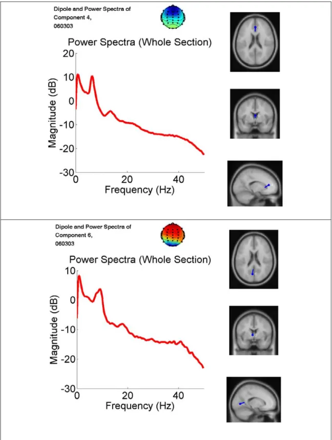
Figure 3-7: An example of the dipole fitting result and the IC spectra. ... - 19 -

Figure 3-8: Component selection procedure. ... - 20 -

Figure 3-9: The smoothed EEG power spectral analysis procedure. ... - 21 -

Figure 3-10: The procedure of component clustering analysis. ... - 23 -

Figure 3-11: The relation between single subject comodulation analysis and component clusters. Different subject has different components.. ... - 25 -

Figure 3-12: The independent modulator decomposition procedure.. ... - 26 -

Figure 3- 13: Method of plotting the frequency weights of the components from each subject for the theta-beta modulator.. ... - 27 -

Figure 3-14: An example of the sorted spectral analysis. ... - 28 -

Figure 4-1: The plots of sorted trials by response time of each subject. ... - 29 -

Figure 4-2: The single subject results of performance change accompanying the component power changes.. ... - 32 -

Figure 4-3: Equivalent dipole source location, spectra and scalp maps for independent component clusters of frontal cluster. ... - 33 -

Figure 4-4: Equivalent dipole source location, spectra and scalp maps for independent component clusters of occipital cluster. ... - 33 -

Figure 4-5: Equivalent dipole source location, spectra and scalp maps for independent component clusters of right motor cluster. ... - 34 -

Figure 4-6: Equivalent dipole source location, spectra and scalp maps for independent component clusters of left motor cluster. ... - 34 -

(8)

Figure 4-8: Representative independent modulation patterns from one subject.. ... - 36 -

Figure 4-9: The normalized frequency patterns of two stable modulators related to alertness changes in each cluster. ... - 38 -

Figure 4-10: The performance changes related to two IM activities of subject 1. ... - 39 -

Figure 4- 11: The performance changes related to two IM activities of subject 2. ... - 39 -

(9)

List of Tables

Table 2-1: NuAmps Specifications ... - 11 - Table 4-1: Subject list ... - 30 - Table 4-2: The correlation coefficients between two modulators and the LDE ... - 43 -

(10)

1. Introduction

1.1 Brain Dynamics in Neural System

Neural systems operated in various dynamic states that determined how they process cognitive information (Livingstone and Hubel, 1981; Kisley and Gerstein, 1999). Cortical electrical activity reflected the different behavioral states that comprise the wake–sleep cycle in higher vertebrates (Caton, 1875; Berger, 1929; Timo-Iaria et al., 1970). These electrical activations were produced by the release of several neuromodulators in the thalamus and cortex. For instance, during arousal, cells in the brainstem laterodorsal tegmentum increased their firing rates (Steriade et al., 1990), releasing acetylcholine in the thalamus (Williams et al., 1994), which depolarized thalamocortical neurons (McCormick, 1992), increasing their firing rates in the tonic firing mode and enhancing the transmission of low-frequency sensory inputs through the thalamus (Singer, 1977; Steriade et al., 1997; Sherman and Guillery, 2001). The postsynaptic depolarization of thalamocortical neurons during arousal also strongly facilitates the transmission of high-frequency sensory inputs through the thalamus (Castro-Alamancos, 2002a), which were normally filtered during quiescent states.

When subjects dropped asleep or drowsiness, most subjects ignored the stimulus from environment and then reduced the influences in brain activity by environment through thalamus gate (Castro-Alamancos., 2002b; Miller et al., 2000) or breakdown of cortical effective connectivity (Massimini et al., 2005).

1.2 Alpha and Theta Rhythm

The frequency of the EEG rhythmic activities may reflect both intrinsic membrane properties of single neurons and the organization and interconnectivity of networks. Lopes da Silva had shown that both thalamo-cortical as well as cortico-cortical loops played an

(11)

Silva, 1991).

Alpha rhythm is the first defined EEG rhythm (Berge, 1929) which power increase is an electrophysiological correlated with cortical idling (Laufs et al., 2003; Robin et al., 2002; Pfurtscheller et al., 1996). These studies showed that alpha power increase accompanied with the decline of the performance (Parikh et al., 2004; Schier., 2000). Theta rhythm is the EEG characteristic of sleep stage 1 and microsleep (Bear et al., 2001; Gennaro et al., 2001). Degradation in performance is also correlated with increased EEG theta power (Beatty et al., 1974; Lal et al., 2002; Takahashi et al., 1997). Moreover, the performance accompanied with the ascension of the alpha and theta activities (Campagne et al., 2004; Keckluno et al., 1993).

1.3 Locations of the EEG Activities Accompanying Cognitive-state Changes

Several studies have shown the EEG power spectra at various scalp locations are correlated with drowsiness in various sustained-attention experiments. The occipital and parietal are the principal areas of scalp that EEG activities accompany changes with performance (Beatty et al., 1974; Parikh et al., 2004; Campagne et al., 2004). Few studies also reported the similar phenomena in the frontal and central regions of the scalp (Schier., 2000; Takahashi et al., 1997). Recently, we applied ICA to multi-channel EEG, and the EEG results showed that component power spectral fluctuations of several components primarily projected to the frontal, central, occipital and parietal scalp locations all exhibited high correlations with the changes in task performance (Lin et al., 2006; Huang et al., 2008).

1.4 Aims of this thesis: Modulators in the Brain Dynamics

Inspired by Onton and Makeig (2007), we hypothesize that there seems to be modulators mediated spectral activations of the cortical areas by intra-cortical feedback loops, or

(12)

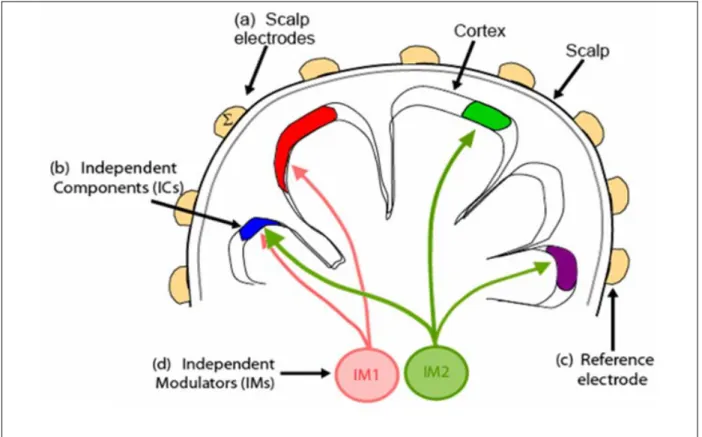
controlled by thalamo-cortical feedback loops. These modulators influence EEG sources influenced by a sub-cortical influence, such as norepinephrine, serotonin, etc. This study investigates the comodulation of the neural system from alertness to drowsiness in a realistic virtual-reality based driving environment to understand the interactions among different cortical areas. The basic principle is shown in Fig. 1-1.

Figure 1-1: The basic principle of neuromodulation. Our EEG sources, here depicted as colored patches, which can express variable oscillatory activity depending on the circumstance, may be influenced by a sub-cortical influence, such as norepinephrine, serotonin, etc, but here just labeled as IM1. This modulator may influence more than one IC, which expresses the cortical source, since we know that neuromodulators have widespread connections to the cortex. The influence of this modulator might be to encourage oscillations at 9 Hz, for example. Whereas IM2 may encourage a 15 Hz rhythm in a different, but partially overlapping set of ICs. Thus, the blue patch of cortex would express bimodal alpha at 9 and/ or 11 Hz depending on the relative strengths of IM1 and IM2.

(13)

2. Materials and Methods

2.1. Dynamic virtual reality environment

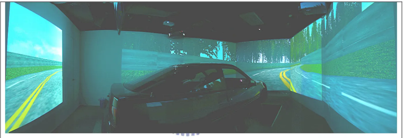
The dynamic VR environment provided a safe, time saving and low cost approach to study human cognition under realistic stimuli. The dynamic VR environment consists of three elements: (1) a six-degree-of-freedom Stewart motion platform; (2) a real car; and (3) a 360-degree 3D VR scene consisting seven projectors. Our driving environment provided not only high-fidelity VR scene, but also kinesthetic inputs and realistic driving environment (as shown in Fig. 2-1). These could make subjects feel that they were driving in a real vehicle on the real road.

Figure 2-1: The overview of the dynamic VR environment, Brain Research Center, National Chiao-Tung University, Taiwan, ROC. The dynamic VR environment consists of three elements: (1) a six-degree-of-freedom Stewart motion platform; (2) a real car; and (3) a 360-degree 3D VR scene consisting seven projectors. The movements of the platform are according to the car dynamics and the condition of the road surface.

2.1.1. VR scene

The VR-based high-fidelity 3D interactive highway scene was developed by using the WorldToolKit (WTK) 3D engine. The 3D view was composed of seven identical PCs running the same VR program and the seven PCs were synchronized by LAN that all scenes were

(14)

corresponding locations.

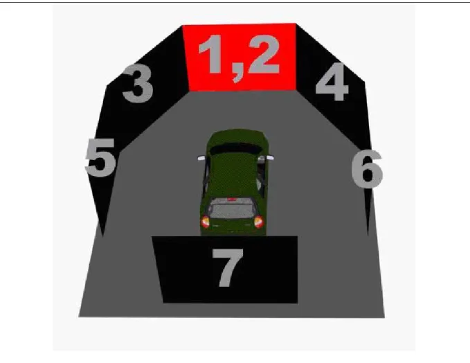
Literatures showed that the horizontal field of view (FOV) of 120° is needed for correct speed perception (Jamson, 2000). In our VR scenes, the surrounded screens covered 206° frontal FOV and 40° back FOV (Fig. 2-2). Frames projected from 7 projectors were connected side by side to construct a surrounded VR scene. The size of each screen had diagonal measuring 2.6-3.75 meters. The vehicle was placed at the center of the surrounded screens.

Figure 2-2: The configuration of the 3D surrounded scene. The 3D VR scene consists of 7 projectors, creating a surrounded view. Frontal screen is overlapped by 2 projector frames in different polarizations, providing a stereoscopic VR scene for 3D visualization.

(15)

2.1.2. Stewart motion platform

The Stewart motion platform had a lower base platform and an upper payload platform connected by six extensible legs with ball joints at both ends (Fig. 2-3). The platform generated accelerations in vertical, lateral and longitudinal direction of vehicle as well as pitch, roll and yaw angular accelerations.

(A) (B) Figure 2-3: (A) A real vehicle (without the unnecessary weight of an engine and other

components) and the platform below the real vehicle. (B) The dynamic platform. A real vehicle was mounted on this platform.

2.2. Subjects

Seventeen right-handed healthy (all males, 18-28 years old) volunteers with normal or corrected to normal vision were paid to participate a lane keeping experiment. All subjects were free from neurological or psychological diseases and without drug or alcohol abuse. No subjects reported with sleep deprivation at one day before the experiment. Subjects were required to have lunch at one hour before the experiment since it has been know that the drowsiness easily occurred during early morning, mid-afternoon, late nights and especially after meal times (Benton et al., 1998).An informed consent were obtained from every subjects before the experiment and the experiment protocol was approved by the Institutional Review Broad of Taipei Veterans General Hospital.

(16)

2.3 The Lane Keeping Driving Task

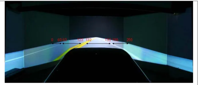
Subjects were instructed to perform a lane-keeping driving task. In this task, the car cruised with a fixed velocity of 100 km/hr on the VR-based highway scene and it was randomly drifted either to the left or to the right away from the cruising position with a constant velocity. The participants were instructed to steer the vehicle back to the center of the cruising lane as quickly as possible when they detected a drifting event. Fig 2-2 shows the time course of a typical deviation event that embedded in the lane-keeping driving task. About 5 to 10 seconds after the system detected the subjects’ response, the next trial started. When subjects fall drowsy, they often exhibit relative inattention to environments, eye closure, less mobility, failure to motor control and making decision (Brookhuis et al., 2003). Since the response time will increases when subjects falling drowsiness, there is linear relationship between response time and deviation. So the vehicle trajectories (driving error) were defined as the basic drowsiness index in the experiment. The VR-based four-lane straight highway scene was applied in the experiment. In this scene, the four lanes from left to right are separated by a median stripe and the distance from the left side to the right side of the road was equally divided into 256 points indicating the position of the vehicle as the digital output signal of the VR scene at each time instant as shown in Fig 2-4. The width of each lane and the car is 60 units and 32 units, respectively. Fig 2-5 shows an example of the driving performance represented by the vehicle deviation trajectories.

(17)

Figure 2-4: The digitized highway scene. The width of highway is equally divided into 256 units and the width of the car is 32 units.

Deviation Onset Reaction Time Cruising (Trajectory) Deviation Response Offset Response Onset Cruising (Trajectory) Res pon_se Time Deviation Onset Reaction Time Cruising (Trajectory) Deviation Response Offset Response Onset Cruising (Trajectory) Res pon_se Time

Figure 2-5: An example of the deviation event. The car cruised with a fixed velocity of 100 km/hr on the VR-based highway scene and it was randomly drifted either to the left or to the right away from the cruising position with a constant velocity. The subjects were instructed to steer the vehicle back to the center of the cruising lane as quickly as possible.

(18)

2.4 EEG Data Acquisition

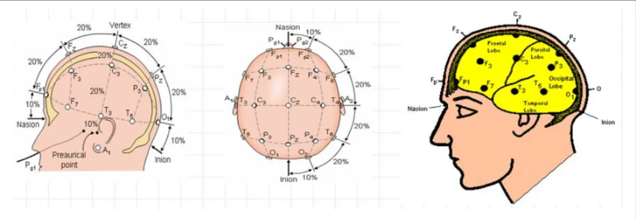
Thirty-two channel EEG signals (using sintered Ag/AgCl electrodes and reference was the mean of the left and right mastoid electrodes ), and one 8-bit digital signal representing the driving performance produced from VR scene were simultaneously recorded by the Scan NuAmps Express system (Compumedics Ltd., VIC, Australia). Fig 2-6 shows the 32 channel EEG electrode cap. All EEG channels were located based on a modified International 10-20 system as shown in Fig 2-7 and Fig 2-8. The 10-20 system is based on the relationship between the locations of an electrode and the underlying area of cerebral cortex. Before acquiring EEG data, the contact impedance between EEG electrodes and the skin was calibrated to be less than 5kΩ by injecting NaCl based conductive gel. The EEG data were recorded with 16-bit quantization levels at a sampling rate of 500 Hz.

(19)

Figure 2-8: The 10-20 international electrode placement system.

Figure 2-7: The International 10-20 system of electrode placement for 32 electrodes, including the lateral view and top view.

(20)

Table 2-1: NuAmps Specifications

Analog inputs 40 unipolar (bipolar derivations can be computed) Sampling frequencies 125, 250, 500, 1000 Hz per channel

Input Range ±130mV

Input Impedance Not less than 80 MOhm

Input noise 1 µV RMS (6 µV peak-to-peak)

Bandwidth 3dB down from DC to 262.5 Hz, dependent upon sampling frequency selected

(21)

3. Data Analyses

3.1. Analysis of driving performance

In each session, deviation trajectory was recorded at 60 Hz, and we can retrieve the deviation onset latency and response onset latency. Similar to real-world driving experience, the vehicle did not always return to the same cruising position after each compensatory steering maneuver. Therefore, during each drift/response trial, driving error was measured by maximum absolute deviation from the previous cruising position (Fig. 3-1).

Figure 3-1: An example of the driving trajectory, recorded with 653 deviation events in a 100-min session. Blue lines: raw trajectory. Green dots: deviation onsets. Red dots: response onsets.

(22)

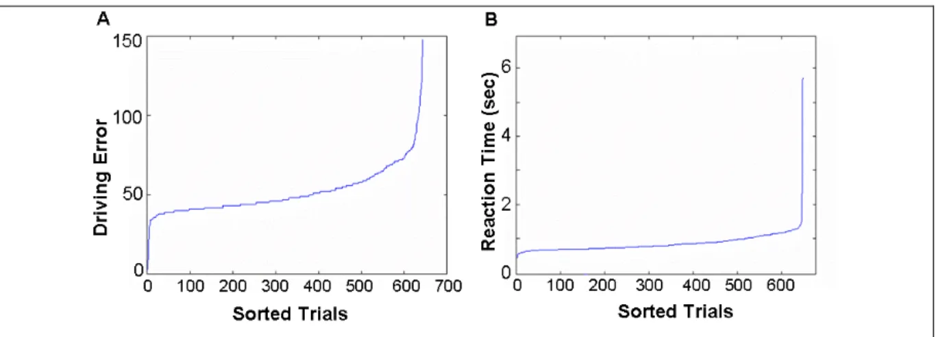
Figure 3-3: (A) Sorted trials by driving error (point). (B) Sorted trials by response time (sec). Since the car drifted with constant velocity, the relation between response time and the driving error was linear (D=c T, c = 60). After transformed the local driving error into response time, behavior responses were sorted by response time, and then plotted as Fig.3-3.

The response time and local driving error were varied along with drivers’ alertness and drowsiness. We had two equal drowsiness indices: response time and the local driving error. For instance, when the driver was drowsy, the response time between the onset of deviation and steering wheel was increased. On the contrary, when the driver was alter, the response time between the onset of deviation and steering wheel was decrease.

Figure 3-2: (A) Driving trajectory of a 100-min session. (B) The local driving error of a 100-min session. It was obtained from the driving trajectory through 4 steps: baseline removal, compute the absolute value, set a threshold, and moving average.

(23)

Since the cruising center was set on the third lane of the highway scene, a threshold (85 pixel) was selected for absolute trajectory to eliminate the diversity of maximum deviation between the vehicle drifted to the left and right. Since the alertness level fluctuates with cycle lengths longer than 4 minutes (Makeig et al., 1996, 2000), we smoothed the trajectory time series by using a causal 90-second square moving-averaged filter to eliminate variances at cycle lengths shorter than 1–2 minutes. The smoothed driving error was called local driving error (LDE) that is linearly correlated with response time. Since subjects easily exhibited relative inattention to environments, eye closure, less mobility, slow or worse motor control or responses or decision making (Brookhuis et al., 2003 ), the LDE was varied along with drivers’ alertness and drowsiness. Therefore, we had a drowsiness index: local driving error. For instance, when the driver was drowsy, the local driving errors were increased. In the contrary, the local driving errors were decreased when the driver was alert.

3.2. EEG

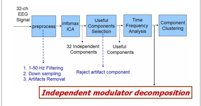
The flow chart of the EEG signal analysis procedure is show in Fig. 3-4. It consists of preprocess, independent component analysis, useful component selection, time-frequency analysis, component clustering, and independent modulator decomposition. All the EEG data were analyzed by using MATLAB and EEGLAB.

(24)

Figure 3-4: The flow chart for the EEG signals analysis procedure. It consists of preprocess, independent component analysis, useful component selection, time-frequency analysis, component clustering, and independent modulator decomposition. All the EEG data were analyzed by using MATLAB and EEGLAB.

3.2.1. EEG Preprocess

The acquired multi-channel EEG signals were first down sampled (from 500 to 250 Hz). A 500-pt high pass filter with a cut-off frequency at 0.5 Hz is used to remove breathing artifacts, and the DC drifts. The width of the transition band of the high pass filter is 0.2 Hz. A 30-pt low pass filter is then applied to the signal with the cut-off frequency at 50 Hz to remove muscle artifacts and line noise. The transition band width of the low pass filter is 7 Hz. The artifacts across all channels were then identified and rejected from EEG data by visual inspection using the EEGLAB visualization function pop_eegplot(). The rejection strategy was to reduce the extreme values data, abnormal electrode activities, and strong muscle artifacts.

(25)

3.2.2. Independent Component Analysis (ICA)

ICA methods have been extensively applied to the blind source separation problem and also demonstrated that was a suitable solution to the problem of EEG source segregation, identification, and localization. (Lee et al., 1999; Jung et al., 2000, 2001; Naganawa et al., 2005; Liao et al., 2005). In this study, we used a version of the infomax algorithm of Sejnowski et al. Firstly, we used ICA to decompose EEG signals into various temporally statistical independent activations (ICA components) and then excluded the artifact based on the time course signals, scalp maps and power spectra of components (Jung et al., 2000; Onton et al., 2006). IC activations from each subject were first assessed and categorized as brain activity or non-brain artifact (e.g., muscle or line noise, or eye movement activity) by visual inspection of their scalp topographies, time courses and activity spectra. Most artifacts can be rejected in the process of useless components rejection. The effectiveness of eye blinking and other artifacts removal by using ICA had been demonstrated in the Jung et al.’s study. Then we employed the time-frequency analysis, which can measures dynamic changes in amplitude of the broad band EEG frequency spectrum as a function of time. Then we used component clustering method to observe the cross-subjects results.

The Infomax ICA can separate N sources from N EEG channels. The conduction of the EEG sensors is assumed to be instantaneous and linear such that the measured mixing signals are linear and the propagation delays are negligible. We also assume that the signal sources of muscle activity, eye, and, cardiac signals are not time locked to the sources of EEG activity which is regarded as reflecting synaptic activity of cortical neurons. Therefore, the time courses of the sources are assumed to be independent. The task of the Infomax ICA algorithm is to recover a version, of the original sources S by finding a square matrix W that inverts the mixing process linearly and save the identical scale and permutation. For EEG analysis, the

(26)

the output data matrix U = WX are time courses of activation of the ICA components, and the columns of the inverse matrix W-1 give the projection strengths of the respective components onto the scalp sensors. The scalp topographies of the components provide information about the location of the sources (e.g., eye activity should project mainly to frontal sites, and the visual event-related potential is on the center to posterior area, etc.). Discarding the sources of muscle activity, eye movement, eye blinking, and single electrode noises, we obtained useful components to do further analysis. Fig. 3-4 shows the ICA decomposition results of single subject.

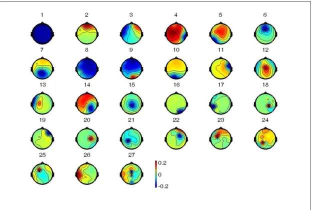
Figure 3-5: The statistical independent activations (components) from the EEG signal decomposed by ICA. 30 sources are separated from 30 EEG channels in the figure.

(27)

Figure 3-6: An example of ICA decomposition. The scalp topographies of ICA weighting matrix by spreading each element of weight into the plane of the scalp which is corresponding to the ICA components based on international 10-20 system.

3.2.3. Independent Component Selection and Dipole Fitting

IC activations from each subject were first assessed and categorized as brain activity or non-brain artifact (e.g., muscle or line noise, or eye movement activity) by visual inspection of their scalp map, activity spectra, and dipole fitting location. ICs were selected by observations and large reduced the number of components into around half by rejecting the noisy components (Fig. 3-8).

DIPFIT2 routines from EEGLAB were then used to fit single dipole source models to the remaining IC scalp topographies using a fourshell spherical head model (Oostenveld and Oostendorp, 2002). In the DIPFIT2 software, the spherical head model is co-registered with an average brain model (Montreal Neurological Institute) and returns approximate Talairach coordinates for each equivalent dipole source. Fig. 3-7 shows the dipole fitting result and the

(28)

Figure 3-7: An example of the dipole fitting result and the IC spectra. DIPFIT2 routines from EEGLAB were then used to fit single dipole source models to the remaining IC scalp topographies using a fourshell spherical head model.

(29)

Figure 3-8: Component selection procedure. IC activations from each subject were first assessed and categorized as brain activity or non-brain artifact (e.g., muscle or line noise, or eye movement activity) by visual inspection of their scalp map, activity spectra, and dipole fitting location, and then reject all components of non-brain artifacts. In this example, red line shows the rejected components.

3.2.4. Time frequency analysis

The processing flow of time frequency analysis was shown in Fig. 3-5. The time sequence of EEG channel data or ICA activations were subject to Fast Fourier Transform (FFT) with a 500-point window with 250-point overlap. Windowed 500-point epochs were further subdivided into several 125-point subwindows with 25-point step. Each 125-point frame was extended to 512 points by zero-padding to calculate its power spectrum by using a 512-point fast Fourier transform (FFT), resulting in power-spectrum density estimation with a frequency resolution near 0.5 Hz. A moving median filter was then used to average and minimize the presence of artifacts in the EEG records of all sub-windows. Previous reports

(30)

linearly in the logarithmic scale than in the linear scale (Bear et al., 2001; Gennaro et al., 2001). Thus, the power spectra of IC activations were further converted into a logarithmic scale. The resultant time series of log power spectra for each session consisted of the power spectra of the IC activations across 20 frequencies (from 1 to 20 Hz) stepping at 2-second (500-point, an epoch) time intervals.

Figure 3-9: The smoothed EEG power spectral analysis procedure. The EEG data of the extracted ICA components was first accomplished using a 750-point Hanning window with 250-point overlap. Windowed 750-point epochs were further subdivided into several 125-point subwindows using the Hanning window again with 25-point step. Each 125-point frame was extended to 256 points by zero-padding to calculate its power spectrum by using a 256-point fast Fourier transform (FFT), resulting in power-spectrum density estimation with a frequency resolution near 1 Hz.

(31)

3.2.5. Component clustering

In order to discover the corss-subjects results, we employed the component clustering analysis after doing ICA decomposition. ICs were first selected by observations and large reduced the number of components into around half by rejecting the noisy components (Fig. 3-8). Then, the selected ICs were first clustered semi-automatically based on the gradients values of the component scalp maps, dipole source locations, power spectra, and within-subject consistency (Onton et al., 2006) by K-mean algorithm. The K-means clustering is to classify or to group objects based on attributes/features into K number of groups. K is a positive integer number. The grouping is done by minimizing the sum of squares of distances between the data and the corresponding cluster centroid as:

2

∑

− = i i k k

x

y

e

(5) where e represent the square error, k x andi y represent the data point and cluster centers, k

(32)

Figure 3-10: The procedure of component clustering analysis. Components of each subject were assessed and categorized as brain activity or non-brain artifact by component selection procedure. The selected components of all volunteer were clustered semi-automatically based on the gradients values, [Gxi Gyi], of the component scalp maps by K-mean algorithm based on the gradients values of the component scalp maps, dipole source locations, power spectra, and within-subject consistency. PSD is the power spectral density of components, and the dipole fitting result was generated by DIPFIT2.

(33)

3.2.6. Independent modulator (IM) decomposition

Here, we present first results of a new method for decomposing fluctuations in the selected independent component (IC) power spectra into independent modulators. The method was applied to the selected IC activity spectra from each subject. Mean logarithmic power at each frequency was subtracted from each single window power spectral estimate. The resulting time series of logarithmic spectral deviations were then concatenated, giving a matrix of size (f 　c, t), where f the number of frequency bins, c the number of subject ICs, and t is the number of time windows. For each subject, this matrix was reduced to its first 10 principal dimensions by PCA. The dimension-reduced log spectral data were then decomposed by infomax ICA to find independent modulators of log spectral power across subsets of time windows within all ICs. Infomax ICA finds a matrix, W, that linearly unmixed the IC spectral activations, x, into a sum of maximally temporally independent, and spatially fixed modulators, u, such that u = Wx. The rows of the resulting ‘activation’ matrix, u, are the independent modulator activations, and its columns, the time points of the input data. Columns of the inverse matrix, W-1, give the relative projection weights from each

independent modulator to each frequency bin of each component. The projection weights, which are the frequent patterns, of the modulator provide information about the modulating frequencies of the modulator.

Fig.3-11. shows the relation between single subject comodulation analysis and component clusters. Different subject has different components. For example, S4 in this figure has only component of frontal. Then we fill in a 'V' marks in the grid of the frontal scalp map. It shows that the mean cluster maps are inserted in the 1st row. Then we take the spectral activates of the selected components to do single subject comodulation analysis. The procedure of the single subject comodulation analysis is shown in Fig. 3-12.

(34)

Figure 3-11: The relation between single subject comodulation analysis and component clusters. Different subject has different components. For example, S4 in this figure has only component of frontal. Then we fill in a 'V' marks in the grid of the frontal scalp map. It shows that the mean cluster maps are inserted in the 1st row. Then we take the spectral activates of the selected components to do single subject comodulation analysis. The procedure of the single subject comodulation analysis is shown in Fig. 3-12.

(35)

Figure 3-12: The independent modulator decomposition procedure. The independent modulator decomposition procedure can be divided into five steps. First, the selected dipolar ICs is divided into 1s windows FFT window power spectra then transformed to log power. Each colored trace represents the power spectrum for a single 1s window. The thick black line is the mean power spectrum of all windows. Third, the mean is removed from each power spectrum. Forth, these data is converted into matrix format. We concatenate this tall matrix from one IC with the same sort of information from all the other selected components, and then we have a matrix of dimensions 'spectra (or frequencies)' by 'spectral windows'. This matrix was then submitted to PCA for dimension reduction to 10 dimensions and then to ICA to find independent spectral modulators from the mean across these selected components. Each row is an IC and each column in this illustration is an IM. What come out of this decomposition are projection weights of 10 independent modulators. The projection weights, which are the frequent patterns, of the modulator provide information about the modulating frequencies of the modulator.

(36)

Fig. 3-13 shows how to plot the frequency weights of the components from each subject for 1 of the modulator. As described in Fig.3-11, it’s needed to fill up the table. In this figure 'V' marks means the frequency weight of each component and the mean frequency weight is plotted by red thick line.

Figure 3- 13: Method of plotting the frequency weights of the components from each subject for the theta-beta modulator. In this figure 'V' marks means the frequency weight of each component and the mean frequency weight is plotted by red thick line.

(37)

3.2.7. LDE-Sorted IM activation analysis and statistical analysis

In order to find the inter-subject relationships between the IM activations and the alertness level, the LDE-sorted analysis method was applied to the IM activation across subjects. The method sorts the smoothed IM activations according to the LDE index to assess the brain dynamics corresponding to the transition from lower LDE to larger LDE. For group analysis, we assumed the alertness levels of all subjects in the lowest LDE states were the same and the difference of the lowest LDE values corresponding to different subjects are caused by the individual reaction speed. To compare the modulator power for the high and slow local driving error across subjects, a paired-sample Wilcoxon signed rank test (signrank, Matlab statistical toolbox, Mathworks) was applied. The significant onset of the alpha increase was earlier than that of the theta increase. All statistical comparisons in this study, a significant level was set at p <0.05.

Figure 3-14: An example of the sorted spectral analysis. The left subplot of Fig 3-6 is a subject’s original LDE trajectory (the blue line) and the corresponding modulator power changes (the red line). The right subplot sorts the LDE values in ascending order and shows the transient modulator powers corresponding to the sorted LDE values. It can be found that the modulator power is increasing at the beginning and will decrease at the latter when LDE values are ascending.

(38)

4. Results

4.1. Behavior performance

All subjects’ LDE were ranged from 0 to 65 units, indicated that subjects got drowsiness in our experimental paradigm. Fig. 4-1 shows the plots of the sorted trials by response time in each subject. The performance was changes almost continuously, and we can analyze the EEG power changes accompany with LDE variations continuously.

(39)

Table 4-1: Subject list

SUBJECT No.

Exp.Time

Sex

Age

Platform State

SUBJECT 1

06/02/27

Male

23 motionless

SUBJECT 2

06/03/03

Male

24 motionless

SUBJECT 3

06/03/08

Male

25 motionless

SUBJECT 4

06/06/29

Male

26 motionless

SUBJECT 5

06/07/06

Male

25 motionless

SUBJECT 6

06/07/07

Male

25 motionless

SUBJECT 7

06/07/10

Male

29 motionless

SUBJECT 8

06/07/11

Male

29 motionless

SUBJECT 9

06/07/25

Male

23 motionless

SUBJECT 10

06/10/31

Male

25 motionless

SUBJECT 11

06/11/01

Male

25 motionless

SUBJECT 12

06/11/02

Male

23 motionless

SUBJECT 13

06/11/30

Male

24 motionless

SUBJECT 14

07/01/02

Male

24 motionless

SUBJECT 15

07/01/05

Male

23 motionless

SUBJECT 16

07/01/17

Male

23 motionless

(40)

4.2. Component spectral fluctuations related to performance changes

The grand results show that the trends of alpha and theta power changes from good performance to poor performance were similar between different brain regions. The performance changes are shown in Fig. 4-2. From the above result, we compared the EEG fluctuations in time series between different components of intra-subject to confirm that the drowsiness related alpha and theta rhythm in these components may be modulated by the same nucleus or synchronized by cortical-cortical interaction. ICA power fluctuations of parietal, occipital, frontal and central components in time series were shown in the Fig. 4-2. The result shows that the alpha power fluctuation of parietal component was highly correlated with the fluctuation of occipital component. Additionally, the theta power fluctuations of frontal, parietal and central component were highly correlated with each other.

(41)

Figure 4-2: The single subject results of performance change accompanying the component power changes. It shows that the trends of alpha and theta power changes from good performance to poor performance were similar between different brain regions. Hence, we compared the EEG fluctuations in time series between different components of intra-subject to confirm that the drowsiness related alpha and theta rhythm in these components may be modulated by the same nucleus or synchronized by cortical-cortical interaction. Scalp maps on the bottom right show the ICA power fluctuations of parietal, occipital, frontal and central components in time series. The result shows that the alpha power fluctuation of parietal component was highly correlated with the fluctuation of occipital component. Additionally, the theta power fluctuations of frontal, parietal and central component were highly correlated with each other.

4.3. Component clustering results

We clustered all components of 17 subjects into 7 groups, and showed the remarkably meaningful and consistent 5 clusters from Fig. 4-3 to Fig.4-7, with the averaged scalp maps, each scalp map and the dipole source locations in the clusters. Where Fig. 4-3 shows frontal cluster, Fig.4-4 shows occipital cluster, Fig. 4-5 shows right motor cluster, Fig. 4-6 shows left motor cluster, and Fig. 4-7 shows parietal cluster. The results of clustering analysis and dipole fitting displayed that most of the brain areas involved in the lane-keeping driving task. These cluster are more remarkable and stable between different participants in the lane-keeping driving task. Hence, only the components that include in these cluster clusters were for further analysis.

In each figure, equivalent dipole source location, spectra and scalp maps for independent component clusters are shown. Scalp maps are shown on the top. Dipole source location is shown on the bottom right. Spectra are shown on the bottom left.

(42)

Figure 4-3: Equivalent dipole source location, spectra and scalp maps for independent component clusters of frontal cluster.

Figure 4-4: Equivalent dipole source location, spectra and scalp maps for independent component clusters of occipital cluster.

(43)

Figure 4-5: Equivalent dipole source location, spectra and scalp maps for independent component clusters of right motor cluster.

Figure 4-6: Equivalent dipole source location, spectra and scalp maps for independent component clusters of left motor cluster.

(44)

Figure 4-7: Equivalent dipole source location, spectra and scalp maps for independent component clusters of parietal cluster.

4.4. Single Subject Independent modulator (IM) decomposition Results

In the section, we discuss the decomposition results of independent modulator. In Fig.4-8., representative independent modulation patterns from one subject. IM window weights and frequency characteristics derived by multiplying the series of spectral deviations from the mean in each 1-s overlapping time window with the PCA/ICA unmixing matrix. Each row represents a computed IC, and each column an IM. The figure shows that IM1 modulated all ICs in alpha-band, and IM2 modulated all ICs in theta-beta-band. The leftmost row shows the IC scalp maps, and top column, the IM window weight histograms. The numbers in the bottom are the correlation coefficient between IM activation and LDE.

(45)

Figure 4-8: Representative independent modulation patterns from one subject. IM window weights and frequency characteristics. It is derived by multiplying the series of spectral deviations from the mean in each 1-s overlapping time window with the PCA/ICA unmixing matrix. Each row represents a computed IC, and each column an IM. The figure shows that IM1 modulated all ICs in alpha-band, and IM2 modulated all ICs in theta-beta-band. The leftmost row shows the IC scalp maps, and top column, the IM window weight histograms. The numbers in the bottom are the correlation coefficient between IM activation and LDE.

(46)

4.5. Frequency characteristics of the independent modulators

Fig. 4-9 shows the normalized frequency patterns of two stable modulators in each cluster. Top panels in Fig. 4-9 show the averaged scalp maps of the clusters, which we obtained in component clustering. Middle panels in Fig. 4-9 display frequency characteristics of the one stable modulator, and bottom panels in Fig. 4-9 exhibit another one. The modulated frequency patterns of corresponding ICs were derived from the column of the inverse matrix, W-1, during the procedure of single subject Independent modulator (IM) decomposition. We normalized the frequency characteristics to observe the common characteristic of each IM. The thin red lines in Fig. 4-9 indicate the modulating frequency of the IM to each component, and the thick red lines in Fig. 4-9 indicate the averaged frequency characteristics of the IM in the cluster. The IMs in middle panels of Fig. 4-9 modulate the theta band, and reveal a peak near 15 Hz in the patterns. This theta dominant modulator affected all areas in our experiment design. The IMs in bottom panels of Fig. 4-9 demonstrate the alpha band modulated in very wide areas.

(47)

Figure 4-9: The normalized frequency patterns of two stable modulators related to alertness changes in each cluster. Top panels show the averaged scalp maps of the clusters. Middle panels display frequency characteristics of the one stable modulator, and bottom panels exhibit another one. The modulated frequency patterns of corresponding ICs were derived from the column of the inverse matrix, W-1 , during the procedure of single subject Independent modulator (IM) decomposition. We normalized the frequency characteristics to observe the common characteristic of each IM. The thin red lines indicate the modulating frequency of the IM to each component, and the thick red lines indicate the averaged frequency characteristics of the IM in the cluster. The IM in middle panels modulate the theta band, and reveal a peak near 15 Hz in the patterns. This theta dominant modulator affected all areas in our experiment design. The IM in bottom panels demonstrate the alpha band modulated in very wide areas.

4.6. Independent modulator activities accompanying performance changes

Fig. 4-10 to Fig.4-16 show the two IM activities related to performance changes. First, we compared the intra-subject fluctuations of two IMs which may be modulated by the nucleus or synchronized by cortical-cortical interaction in time series during different alertness levels to confirm that the alpha and theta-beta modulator related drowsiness level. Letter a-c shows the fluctuations of the LDE, theta-beta modulator, and alpha modulator for two subjects in time series. In Fig. 4-10 to Fig.4-15, (a) exhibits the changes of the LDE during whole experiment, and (b) is the fluctuations of the theta-beta modulator, and (c) shows the fluctuations of the alpha modulator. The theta-beta modulator fluctuates very little during the low LDE periods, and increases monotonically from low LDE to high LDE. Different with the theta band, the alpha modulator fluctuates very large during the low LDE periods. The correlation results between the LDE and two modulators of each subject were

(48)

Figure 4-10: The performance changes related to two IM activities of subject 1.

(49)

(50)

(51)

Figure 4-16: The LDE-Sorted IM activation on two IM activations of all subjects. It showed the mean and SD of the two LDE-sorted IM activations. Fig. 4-16a displays the result of the LDE-Sorted theta-band dominant IM activation, and LDE-Sorted theta-beta modulator activity was significantly increases monotonically from low LDE to high LDE, and the LDE-Sorted alpha modulator, which shows in Fig. 4-16b, was remarkably increases and then sustains from low LDE to high LDE. Additionally, we observed the variances of the two IM activities in the same value of LDE across 17 subjects. The variations were very small in all participants, revealing that the results of the LDE-sorted have inter-subject consistence.

(52)

Table 4-2: The correlation coefficients between two modulators and the LDE SUBJECT No. Theta-Beta Modulator Alpha Modulator

SUBJECT 1 0.7861 0.5713 SUBJECT 2 0.7845 0.6093 SUBJECT 3 0.9433 0.2002 SUBJECT 4 0.8689 0.6619 SUBJECT 5 0.7783 0.5189 SUBJECT 6 0.8201 0.6162 SUBJECT 7 0.9228 0.029 SUBJECT 8 0.8715 0.2748 SUBJECT 9 0.7722 0.3341 SUBJECT 10 0.7957 0.2485 SUBJECT 11 0.8043 0.0831 SUBJECT 12 0.8427 0.683 SUBJECT 13 0.818 0.1898 SUBJECT 14 0.7174 0.5748 SUBJECT 15 0.9282 0.6457 SUBJECT 16 0.9337 0.6186 SUBJECT 17 0.7641 0.5353 Mean Value 0.83246 0.43497 Standard Deviation 0.06812 0.22137

(53)

5. Discussion

5.1 The component spectral fluctuations related to performance

The theta and alpha power changes of several components from good performance to poor performance were similar between different brain regions. It is consistent with past studies (Lin et al., 2006; Huang et al., 2008). Hence, we compared the component fluctuations in time series between different components of intra-subject to confirm that the drowsiness related alpha and theta rhythm in these components may be modulated by the same nucleus or synchronized by cortical-cortical interaction.

5.2 The modulatory model of the neural system

The modulatory model underlying this analysis was illustrated schematically in Fig. 1-1. Independent component analysis (ICA) was applied to EEG data to identifies temporally distinct (independent) signals generated by partial synchronization of local field potentials within cortical patches (b) and summing in different linear combinations at each electrode depending on the distance and orientation of each cortical patch from the scalp (a) and reference electrode (c). The spectra of resulting cortical independent components (ICs) monotonically decrease with frequency, on average, but exhibit large and frequent variations across time. These spectral modulations may be modeled as exponentially weighted influences of several near-independent modulator (IM) processes (d) that independently modulate the activity spectra of one or more independent component (IC) signals. On converting the IC spectra to log power, combined IM influences on IC spectra are converted to log-linear weighted sums of IM influences, allowing a second linear ICA decomposition, applied to the IC log power spectra, to separate the effects of the individual IM processes (d) across EEG frequencies and IC sources (b).

(54)

investigate the modulation model. They have examined the correlation between occipital EEG alpha rhythm, selectively extracted using ICA, and fluctuations in the BOLD effect during an open versus closed eyes and an auditory stimulation versus silence condition. Occipital alpha amplitude is consistent with metabolic changes occurring simultaneously, sites in the medial thalamus and in the anterior midbrain, with about 2.5 sec lag. Goncalves et al.(2005) used simultaneous recording of electroencephalogram/functional magnetic resonance images (EEG/fMRI) to identify blood oxygenation level-dependent (BOLD) changes associated with spontaneous variations of the alpha rhythm, which is considered the hallmark of the brain resting state. They also found the BOLD signal was positively correlated with the alpha power in small thalamic areas, supporting the cortical and subcortical modulation of electroencephalographic alpha rhythm.

A combined PET/EEG study by Schreckenberger et al. also supported the hypothesis of a close functional relationship between thalamic activity and alpha rhythm in humans mediated by corticothalamic loops. (Schreckenberger et al., 2004) This functional corticothalamic loop supports the concept of cortical control of thalamic activity in humans for modulating cortical EEG activity.

Physiological processes that may produce these patterns include several brain systems regulating brain and behavioral arousal and/or valuation judgments of stimulus and other events via the release by midbrain or brainstem neurons of modulatory neurotransmitters – dopamine (DA), acetylcholine (ACh), norepinephrine (NE), serotonin, etc. – through their extensive cortical and thalamic projections (Robbins, 1997; Bardo, 1998).

(55)

5.3 The modulator fluctuations from alertness to drowsiness

In this study, we employed independent modulator decomposition to the spectral fluctuations of independent components, and two independent modulators related to performance changes were found in all subjects.

The alpha modulators were very sensitive to the performance changes, so the alpha modulator fluctuates very large during the low LDE periods. Therefore, the alpha modulator in this study might be partially contributed by cortical idling, decreased attentiveness and decline of movements. In the earlier finding (Lee et al., 1999), the frequency of the 8-14 Hz synchronizes in the thalamocortical system during quiet sleep. The EEG fluctuations from low error to high error were similarly during frontal, central-parietal and occipital lobe in the experiment. So that the alpha modulator maybe also modulated by thalamus during drowsiness.

The theta-beta modulators increase monotonically from low LDE to high LDE. Theta rhythm is the EEG characteristic of sleep stage 1 and microsleep (Bear et al., 2001; Gennaro et al., 2001; Thomas et al., 2003). Past studies also reported the fluctuations in the modulation of the beta-wave amplitude related to an indirect measurement of drowsiness (Poupard et al., 2001). Jung et al. (1997) also reported theta and beta band power were high correlated with performance changes.

The correlation coefficient between modulator power change and LDE is shown in Table 4-2. The standard deviation is large because the inter-subject behavior states are varied. Some subjects were involved more period of stage 1 sleep, others included more time of cortical idling, so that results of the independent modulator decomposition depend on drowsiness state.

(56)

6. Conclusions

In this study, we model spectral fluctuations of independent components from EEG activations as the actions of independently modulator processes, and report two main classes of spectral modulation patterns, alpha modulator and theta-beta modulator. The theta-beta modulator fluctuates very little during the low LDE periods, and increases monotonically from low LDE to high LDE. Different with the theta-beta band, the alpha modulator fluctuates very large during the low LDE periods. Therefore, the theta-beta modulator is high correlated with performance changes, and alpha modulator in this study might be partially contributed by cortical idling. In our modulation model, these modulators are modulated by the subcortical nucleus or synchronized by cortical-cortical interaction to influence on the rhythmic activations of cortical areas. The neuromodulatory systems can be explored more by the method we propose here.

(57)

References

Bardo MT, “Neuropharmacological mechanisms of drug reward: beyond dopamine in the nucleus accumbens.” Critical Reviews in Neurobiology, 12,37-67, 1998

Bear MF, Connors BW, Paradiso MA, “Neuroscience: Exploring the brain.” Lippincott Williams and Wilkins, 2001

Beatty J, Greenberg A, Deibler WP, Hanlon JO, “Operant control of occipital theta rhythm affects performance, in a radar monitoring task.” Science, 183, 871-873, 1974

Benton D, Parker PY, “Breakfast, blood glucose, and cognition.” The american journal of clinical nutrition, 67, 772-778, 1998

Berger H, “Uber das Elektroenkephalogramm des menschen.“ Archives of Psychiatric, 87, 527–570, 1929

Brookhuis KA, Waard DD, Fairclough SH, “Criteria for driver impairment.” Ergonomics, 46, 433-445, 2003

Campagne A, Pebayle T, Muzet A, “Correlation between driving errors and vigilance level: influence of the driver’s age.” Physiology & Behavior, 80, 515– 524, 2004

Caton R, “The electric currents of the brain.” British Medical Journal, 2, 278, 1875

Castro-Alamancos MA, “Different temporal processing of sensory inputs in the rat thalamus during quiescent and information processing states in vivo.” Journal of Physiology, 539, 567–578, 2002a

Castro-Alamancos MA, Oldford E, “Cortical sensory suppression during arousal is due to the activity-dependent depression of thalamocortical synapses.” Journal of Physiology, 541, 319–331, 2002b

Delorme A, Makeig, S, “EEGLAB: an open source toolbox for analysis of singletrial EEG dynamics.” Journal of Neuroscience Methods, 134, 9-21, 2004

(58)

correlates of electroencephalographic alpha rhythm modulation.” Journal of Neurophysiology, 93, 2864-72, 2005

Gennaro LD, Ferrara M, Bertini M, “The boundary between wakefulness and sleep: quantitative electroencephalographic changes during the sleep onset period.” Neuroscience, 107, 1-11, 2001

Gonçalves SI, de Munck JC, Pouwels PJ, Schoonhoven R, Kuijer JP, Maurits NM, Hoogduin JM, Van Someren EJ, Heethaar RM, Lopes da Silva FH, “Correlating the alpha rhythm to BOLD using simultaneous EEG/fMRI: inter-subject variability.” Neuroimage, 30, 203-13, 2006

Jung TP, Makeig S, Humphries S, Lee TW, McKeown MJ, Iragui V, Sejnowski TJ, “Removing electroencephalographic artifacts by blind source separation.” Sychophysiology, 37, 163-78, 2000

Jung TP, Makeig S, Stensmo M, Sejnowski TJ, “Estimating alertness from the EEG power spectrum.” IEEE Transactions on Biomedical Engineering, 44, 1, 1997

Jung TP, Makeig S, Westerfield W, Townsend J, Courchesne E, Sejnowski TJ, ”Analysis and visualization of single-trial event-related potentials.” Human brain Mapping, 14, 166-185, 2001

Keckluno G, Akersteot T, “Sleepiness in long distance truck driving: an ambulatory EEG study of night driving.” Ergonomics, 36, 1007-1017, 1993

Kisley MA, Gerstein GL, “Trial-to-trial variability and state dependent modulation of

auditory-evoked responses in cortex.” Journal of Neuroscience, 19, 10451–10460, 1999 Lal KL, Craig A, “Driver fatigue: Electroencephalography and psychological Assessment.”

Psychophysiology, 39, 313-321, 2002

Laufs H, Kleinschmidt A, Beyerle A, Eger E, Salek-Haddadi E, Preibisch C, Krakow K, “EEG-correlated fMRI of human alpha activity.” Neuroimage, 19, 1463-1476, 2003

(59)

Lee TW, Girolami M, Sejnowski TJ, “Independent component analysis using an extended infomax algorithm for mixed sub- and super-Gaussian sources.” Neural computation, 11, 606-633, 1999

Liao R, Krolik JL, McKeown MJ, “An information-theoretic criterion for intrasubject alignment of FMRI time series: motion corrected independent component analysis.” IEEE Transactions on Medical Imaging, 24, 29-44, 2005

Lin CT, Wu RC, Liang SF, Huang TY, Chao WH, Chen YJ, and Jung TP, “EEG-based Drowsiness estimation for safety driving using independent component analysis.” IEEE Transactions on Circuit and System, 52, 2726-2738, 2005

Livingstone MS, Hubel DH, “Effects of sleep and arousal on the processing of visual information in the cat.” Nature, 291, 554 –561, 1981

Lopes da Silva, F.H., ”Neural mechanisms underlying brain waves: from neural membranes to networks.” Electroencephalography and Clinical Neurophysiology, 79, 81-93, 1991 Makeig S, Bell AJ, Jung TP, Sejnowski TJ, “Independent component analysis of

electroencephalographic data.” Advances in neural information processing systems, 8, 145-151, 1996

Makeig S, Jung TP, Sejnowski TJ, “Awareness during Drowsiness: Dynamics and

Electrophysiological Correlates.” Canadian Journal of Experimental Psychology, 54, 266-273, 2000

Massimini M, Ferrarelli F, Huber R, Esser SK, Singh H, Tononi G, “Breakdown of cortical effective connectivity during sleep.” Science, 309, 2228-2232, 2005

McCormick DA, “ Neurotransmitter actions in the thalamus and cerebral cortex and their role in neuromodulation of thalamocortical activity.” Progress in Neurobiology, 39, 337–388, 1992

(60)

journal of neuroscience, 20(18) 7011–7016, 2000

Naganawa M, Kimura Y, Ishii K, Oda K, Ishiwata K, Matani A, “Extraction of a plasma time-activity curve from dynamic brain pet images based on independent component analysis.” IEEE transactions on biomedical engineering, 52, 201–210, 2005

Onton J, Westerfield M, Townsend J, Makeig S, “Imaging human EEG dynamics using independent component analysis.” Neuroscience and Biobehavioral Reviews, 30, 808–822, 2006

Oostenveld, R., Oostendorp, T.F., “Validating the boundary element method for forward and inverse EEG computations in the presence of a hole in the skull.” Human brain Mapping, 17, 179–192, 2002

Parikh P, Tzanakou ME, “Detecting drowsiness while driving using wavelet transform.” Bioengineering Conference Proceedings of the IEEE 30th Annual Northeast, 17-18, 2004

Pfurtscheller G, Stancak A, Neuper CH, ” Event-related synchronization (ERS) in the alpha band-an electrophysiological correlate of cortical idling: A review.” International journal of psychophysiology, 24, 39-46, 1996

Poupard L, Sartène R, Wallet JC, “Scaling behavior in beta-wave amplitude modulation and its relationship to alertness.” Biological Cybernetics, 85, 19-26, 2001

Robbins TW, “Arousal systems and attentional processes.” Biological Psychology, 45, 57-71, 1997

Robin G, John S, Jerome E, Mark C, “Simultaneous EEG and fMRI of the alpha rhythm.” Brain imaging, 13, 2487-2492, 2002

Schier MA, “Changes in EEG alpha power during simulated driving: a demonstration.” International Journal of Psychophysiology, 37, 155-162, 2000

(61)

HG, Bartenstein P, Gründer G, “ The thalamus as the generator and modulator of EEG alpha rhythm: a combined PET/EEG study with lorazepam challenge in humans.” Sherman SM, “Guillery RW Exploring the thalamus.” San Diego, Academic. 2001

Singer W, “Control of thalamic transmission by corticofugal and ascending reticular pathways in the visual system. “ Physiol Rev , 57, 386–420, 1977

Steriade M, Datta S, Pare D, Oakson G, Curro Dossi RC, “Neuronal activities in brain-stem cholinergic nuclei related to tonic activation processes in thalamocortical systems.” Journal of Neuroscience, 10, 2541–2559, 1990

Steriade M, Jones EG, McCormick DA, “Thalamus.” New York: Elsevier.

Takahashi N, Shinomiya S, Mori D, Tachibana S, “Frontal midline theta rhythm in young healthy adults.” Clinical electroencephalography, 28, 49-54, 1997

Timo-Iaria C, Negrao N, Schmidek WR, Hoshino K, Lobato de Menezes CE, Leme da Rocha T, “Phases and states of sleep in the rat.” Physiology and Behavior, 5, 1057–1062, 1970 Williams JA, Comisarow J, Day J, Fibiger HC, Reiner PB, “Statedependent release of

acetylcholine in rat thalamus measured by in vivo microdialysis.” Journal of Neuroscience, 14, 5236–5242, 1994

探討打瞌睡腦波之神經調控機制

國 立 交 通 大 學

網路工程研究所

碩 士 論 文

探討打瞌睡腦波之神經調控機制

Co-modulation of EEG Activity during Drowsiness

研 究 生： 莊 尚 文

指導教授： 林 文 杰 博士

林 進 燈 博士

探討打瞌睡腦波之神經調控機制

Co-modulation of EEG Activity during Drowsiness

研 究 生：莊尚文 Student：Shang-Wen Chuang

指導教授：林文杰 博士

Advisor：Dr. Wen-Chieh Lin

林進燈 博士

Dr. Chin-Teng Lin

國立交通大學網路工程研究所

碩士論文

Augest 2008

Hsinchu, Taiwan, Republic of China

探討打瞌睡腦波之神經調控機制

學生：莊尚文

指導教授：林文杰博士

林進燈博士

中文摘要

Co-modulation of EEG Activity during Drowsiness

Student: Shang-Wen Chuang

Advisor: Dr. Wen-Chieh Lin

Dr. Chin-Teng Lin

Abstract

誌 謝

Acknowledgement

Contents

List of Figures

List of Tables

1. Introduction

1.1 Brain Dynamics in Neural System

1.2 Alpha and Theta Rhythm

1.3 Locations of the EEG Activities Accompanying Cognitive-state Changes

1.4 Aims of this thesis: Modulators in the Brain Dynamics

2. Materials and Methods

2.1. Dynamic virtual reality environment

2.1.1. VR scene

2.1.2. Stewart motion platform

2.2. Subjects

2.3 The Lane Keeping Driving Task

2.4 EEG Data Acquisition

3. Data Analyses

3.1. Analysis of driving performance

3.2. EEG

3.2.1. EEG Preprocess

3.2.2. Independent Component Analysis (ICA)

3.2.3. Independent Component Selection and Dipole Fitting

3.2.4. Time frequency analysis

3.2.5. Component clustering

∑

x

y

e

3.2.6. Independent modulator (IM) decomposition

3.2.7. LDE-Sorted IM activation analysis and statistical analysis

4. Results

4.1. Behavior performance

SUBJECT No.

Exp.Time

Sex

Age

Platform State

SUBJECT 1

06/02/27

Male

23

motionless

SUBJECT 2

06/03/03

Male

24

motionless

SUBJECT 3

06/03/08

國立交通大學

碩士論文

研究生：莊尚文

指導教授：林文杰博士

林進燈博士

研究生：莊尚文 Student：Shang-Wen Chuang

指導教授：林文杰博士

林進燈博士

誌謝