有限理性與彈性迷思：在代理人基計算消費性資本資產定價模型下的分析

Bounded Rationality and the Elasticity Puzzle: Analysis

Based on Agent-Based Computational Consumption

Capital Asset Pricing Models

AI-ECON Research Center Department of Economics National Chengchi University

Taipei, Taiwan 116 E-mail: [email protected]

Abstract

In this paper, we address the influence of bounded rationality on the well-known elasticity puzzle. An agent-based consumption asset pricing model is built upon Chen and Huang (2007a), and time series data of consumption and returns are gen-erated from the the simulations of this model. With this artificial data, we apply standard econometric methods to estimate the elasticity of intertemporal consump-tion for both the systems of individual and aggregate Euler consumpconsump-tion equaconsump-tions. A number of findings may shed light on the empirical study of the elasticity puzzle. First, it is found that the agents’ built-in parameter of the elasticity of intertempo-ral substitution is not able to be discovered by the standard econometric procedure; instead, it can be underestimated, and can be further underestimated by using ag-gregate data. Consequently, by the reciprocal relation, the coefficient of relative risk aversion may be overestimated. Second, agents with better forecasting accuracy, who in turn become wealthier, tend to exhibit higher estimated elasticities than those with worse one, even though they both are are endowed with an identical elasticity. In other words, the observed positive relation between wealth share and intertempo-ral elasticity can be spurious. The role the heterogeneity in risk preference is also analyzed.

Keyword: Bounded Rationality, Elasticity Puzzle, Risk Preference, Consumption Cap-ital Asset Pricing Model, Agent-Based Computational Modeling, Genetic Algorithms

1 Introduction and Motivation

In this paper, an agent-based computational capital asset pricing model is applied to address the issue, known as the elasticity puzzle, originating from a famous reciprocal relation between the elasticity of intertemporal substitution and the relative risk aversion

co-efficient. By the reciprocal relation, the implied relative risk aversion coefficient can be

unexpectedly, and possibly unacceptably, high when the estimated elasticity of intertem-poral substitution is so low and even closer to zero.

Existing studies, be they theoretical or empirical, on the elasticity puzzle are largely confined to the conventional framework built upon the devices of rational expectations and representative agents. A number of recent empirical studies, however, have docu-mented that agents are heterogeneous in their elasticity of intertemporal substitution.1 Two questions immediately arise. The first one concerns the aggregation problem. If the intertemporal elasticity is heterogeneous among agents, then what is the relation be-tween the aggregate elasticity and its individual counterparts? This leads us to the very basic issue raised by Alan Kirman, “whom or what does the representative individual represent?” The second one is why the rich and the stockholders tend to have to high intertemporal elasticities, and their opposites tend to have low ones. Why is such a be-havioral parameter so critical in determining the wealth share of individuals?2

Empirical studies also find that the Euler consumption equation applies well only to the stock market participants, and not to all individuals. It is certainly plausible that not all individuals can do optimization well. So, here comes the third question. Is it possible that some agents who happen to do optimization well and hence behave closer to what the Euler equation predicts eventually become wealthier, and for those who do not and hence fail the Euler equation eventually become poor? Do the rich really have different intertemporal elasticities as opposed to their opposites, or are they just “smarter” or with a better luck? Is that possible the “observed” heterogeneity in intertemporal elasticity is just spurious? In sum, what is the relation between the observable elasticity and the true one, considering that agents are boundedly rational?

Using an agent-based computational model, we study a consumption capital asset pricing model (CAPM, hereafter) composed of boundedly-rational interacting heteroge-neous agents. These agents are heterogeheteroge-neous in their forecasts (the way which they learn from the past), saving and investment decisions, driven by an adaptive scheme, specifically, genetic algorithms. Their preferences can be homogeneous or heteroge-neous, depending on what we are asking. Simulating the model can generate a sequence of time-series observations of individuals’ profiles, including beliefs, consumption, sav-ings, and portfolios. Unlike most theoretical or empirical studies of the consumption CAPM model, the agent-based computational model do not assume an exogenously given stochastic process of returns and consumption. Instead, aggregate consumption, asset prices, and returns are also endogenously generated with agents under specified risk preferences and intertemporal elasticities. With this endogenously generated aggre-gate and individual data, we are better equipped to answer the three questions posed above in a fashion of survival dynamics.

The rest of the paper is organized as follows. We shall first give a little technical review of the elasticity puzzle (Section 2.1), followed by a literature review on the reflections upon the puzzle (Section 2.2). There are basically two kinds of reflections, namely the one from the econometric viewpoint (Section 2.2.1), and the one from the theory view-point (Sections 2.2.2 and 2.2.3). For the latter, we further distinguish the relaxation of the assumption of the power utility function (Section 2.2.2) and the relaxation of the as-sumption of the representative agent (Section 2.2.3). This background knowledge helps

1_{For example, it is found that the intertemporal elasticity is different between the poor and the rich, and} is also different between stockholders and non-stockholders. See the literature review in Section 2.2.3.

2_{The question becomes even more puzzling given the irrelevance theorem of preferences to wealth share.} (Sandroni, 2000; Blume and Easley, 2004)

us define the departure of this paper (Section 2.2.4), which has an agent-based consump-tion Capital Asset Pricing Model (Secconsump-tion 3) as a core. Technical details of the model are left for Appendix A and Appendix B. Based on the proposed agent-based consump-tion CAPM model, Secconsump-tion 4 proposes two experimental designs to examine the effect of bounded rationality on the estimated elasticity, and the results are shown and analyzed in Equation 5. The analysis is econometric and is based on the Euler consumption equa-tion, whose derivation is briefly reviewed in Appendix C. Section 6 then closes the paper with a few concluding remarks.

2 The Puzzle and the Reflections

The elasticity of intertemporal substitution (EIS, hereafter), as a technical characterization of economic behavior and a basic parameter of economic models, plays a pivotal role in economic analysis. To name a few, its magnitude can determine the sensitivity of saving to interest rate, the effect of capital income taxation (Summers, 1981; King and Rebelo, 1990), and the impact of uncertainty on the rate of economic growth (Jones, Mauelli and Stachetti, 1999). Given its significance, a great deal of effort has been devoted to the empirical study of its magnitude.

An early influential empirical finding was established in Hall (1988), which evidences a low or, in fact, an almost zero intertemporal elasticity.

All the estimates presented in this paper of the intertemporal elasticity of sub-stitution are small. Most of them are also quite precise, supporting the strong conclusion that the elasticity is unlikely to be much above 0.1, and may well be zero. (Ibid, p. 340)

This result implies that consumption growth is completely insensitive to changes in interest rates. Hall’s estimation is build upon the consumption capital asset pricing model, originally put forwarded by Breeden (1979). A typical assumption in this model is that preference is intertemporal separable. A significant consequence of making this assump-tion is that the EIS and the risk attitude, the two distinct aspects of preference, are inter-twined. Actually, the EIS and the risk aversion parameter are reciprocals of one another. If we further assume that a representative agent who maximizes the expectation of a time separable power utility function:

ut= E{ ∞

∑

where β is the rate of time preference, ct is the investor’s consumption in period t and

ρ is the coefficient of relative risk aversion. The mathematical expectation E(· |) is

con-ditioned on information available to agents at time t, Ωt. Then the reciprocal relation

becomes simply

ψ = 1

whereψ is the elasticity of intertemporal substitution.

The reciprocal relation puts Hall (1988) in a sharp contrast to Hansen and Singleton (1982, 1983), which is commonly cited for evidence that the (constant) coefficient of rel-ative risk aversion is small. Hall’s estimates suggest that the value of the intertempo-ral elasticity of substitution, i.e. the reciprocal of the parameter estimated by Hansen and Singleton, is much smaller than that implied by any of the Hansen-Singleton esti-mates. The disparity defines an “elasticity puzzle” as phrased by Neely, Roy and White-man (2001), “is the risk aversion parameter in the simple intertemporal consumption CAPM small as in Hansen and Singleton (1982, 1983), or is it that its reciprocal, the in-tertemporal elasticity of substitution, is small, as in Hall (1988)?”3

In a technical way, the elasticity puzzle can be summarized as the conflicts of estimating the same coefficient in two regression equations. The one used in Hall (1988) and many follow-ups is the consumption Euler equation,

Δct= τ + ψrt+ ξt, (3)

whereΔctis the consumption growth at time t, rt+1is the real return on the asset at t, and

τ is a constant. As well discussed by Hall (1988), the time aggregation problem, e.g., using

quarterly data instead of the monthly data, can cause the error ξt be no longer white

noise. Instead, it is linear in the innovation to consumption growth and asset return, and is correlated with the regressor rt. However, given a vector of instruments Zt−1

uncorrelated with the error,ψ can be identified by the moment restriction

E[Zt−1ξt] = 0. (4)

Here Zt−1typically consists of economic variables known at time t− 1, such as lagged

consumption growth and asset return. Equation (3) can be estimated by two-stage least

squares (TSLS) if the error is homoskedastic, or by linear generalized method of moments

(GMM) if the error is heteroskedastic.

Alternatively, the regression equation considered by Hansen and Singleton (1983) is the reversed form of (3):

rt = μ +_ψ1Δct+ ηt = μ + ρΔct+ ηt (5)

where μ is a constant and ηt+1 is the error. The reciprocal of the EIS, which is also the

coefficient of the relative risk aversion ρ under CRRA utility, is then identified by the moment restriction

E[Zt−1ηt] = 0. (6)

The moment restriction (4) and (6) are equivalent up to a linear transformation.

The elasticity puzzle can then be exemplified by a comprehensive study by Camp-bell (2003). CampCamp-bell (2003) gives a very extensive comparison between the estimates of the two equations (3) and (5) by using many different countries’ data. He reports in his Table 9 the results. Consider the case of using quarterly U.S. data (1947-1998) on non-durable consumption and T-bill returns, the 95% interval forψ is [−0.14, 0.28], and for_ψ1

[−0.73, 2.14]. Therefore, one reject the null hypothesis ψ = 1 using equation (3), which in-struments for T-bill return, but fails to rejectψ = 1 using equation (5), which instruments for consumption growth.4

2.2 Reflecting upon the Puzzle 2.2.1 Econometrics

Given this technical description, a natural way to reflect upon the elasticity puzzle is to assume an econometric essence of the puzzle, and instruments Zt seem to attract wide

attention of econometricians. There are at least two major observations made about Zt.

The first observation is related to the choice of normalization for the moment restric-tion. Although equations (4) and (6) correspond to the same moment restriction up to a linear transformation, GMM is not invariant to such transformations. Therefore, the choice of normalization for the moment restriction can affect point estimates and confi-dence intervals. Nonetheless, the conventional asymptotic theory may make the choice of normalization negligible in large samples, leading to the same inference of the EIS. Therefore, the puzzle may be more than just a debate over whether normalization of the key structural equation matters.

The second observation is pioneered by Neely, Roy and Whiteman (2001), which at-tributes the disparate estimates of this fundamental parameter to failures of instrument

relevance. Instruments which are insufficiently correlated with endogenous variables,

also known as weak instruments, can cause estimators to be severely biased and the finite-sample distribution of test statistics to depart sharply from the limiting distribution, lead-ing to large size distortions in hypothesis tests. Neely, Roy and Whiteman (2001) note that weak instruments are a problem in estimating the EIS because both consumption growth and asset returns are notoriously difficult to predict. Because of weak identification, it is imperative, as they suggested, to use prior beliefs grounded in economic theory to settle the debate over small versus large risk aversion.

2.2.2 Economic Theory: Preferences

Back to economic theory, what seems to be immediate relevant is the utility function or risk

attitude upon which the reciprocal relation (2) is built. Consumption asset pricing models

typically assume a power utility function in which the elasticity of intertemporal substi-tution cannot be disentangled from the coefficient of relative risk aversion. Despite the use of a power utility function, Hall (1988) still argues that this specification is inappro-priate because the EIS deals with the willingness of an investor to move consumption between time periods and is well defined even in the absence of uncertainty. In contrast, the coefficient of relative risk aversion concerns the willingness of an investor to move consumption between states of world and is well defined even in a one period model.

Epstein and Zin (1991) has suggested an alternative specification for preference which can disentangle risk aversion from intertemporal substitution. Specifically, the utility

4_{Actually, these numbers are provided by Yogo (2004), and are not directly available from Campbell} (2003).

function can be defined recursively as follows: ut= (1 − β)c 1−ρ θ t + β(Et(u1_t+1−ρ) 1 θ) θ 1−ρ (7) forθ ≡ (1 − ρ)/(1 − 1/ψ) where ψ is the elasticity of intertemporal substitution, ρ and

β, as before, are the coefficient of relative risk aversion and the rate of time preference,

respectively. Whenθ = 1, or alternatively when ρ = 1/ψ, this specification reduces to a time-separable power utility model.

This specification retains many of the attractive features of the power utility function but is no longer time separable. Nonetheless, in spite of the theoretical appeal of the Epstein-Zin specification, empirical tests, such as Epstein and Epstein-Zin (1991) and Smith (1998), have not been successful in disentangling the elasticity of intertemporal substitution from the coefficient of relative risk aversion.

2.2.3 Economic Theory: Heterogeneity

In addition to preference, heterogeneity provides another possibility to reflect upon the puzzle. This is so because one feature common to all the studies which we go through above is their reliance on the representative-agent assumption. The representative-agent assumption says that one can treat the aggregate data as the outcome of a single “repre-sentative” consumer’s decisions. However, as Kirman (1992) has argued, the conditions on individual preferences necessary for the representative agent to be an exact represen-tation of the behavior of underlying agents are quite stringent, so much so as to be im-plausible. Therefore, while the representative agent model is still considered to be useful for analyzing behavior from aggregate data, recent research tendency does indicate a gradual movement towards models of heterogeneous agents by abandoning this device. On the elasticity puzzle, Guvenen (2002) is the one pioneering this direction.

In his analysis, Guvenen shows that the elasticity puzzle arises from ignoring two kinds of heterogeneity across individuals, namely, heterogeneity in wealth and hetero-geneity in the EIS. For the first heterohetero-geneity, there is substantial wealth inequality in the U.S., and 99 percent of all the equity is owned by 30 percent of the population. Obviously, a large fraction of U.S. households do not participate in stock markets. On the other hand this group’s contribution to total consumption is much more modest: the top 10 percent wealthy account for around than 17 percent of aggregate consumption. As to the second heterogeneity, a variety of microeconomic studies using individual-level data conclude that an individual’s EIS increases with his wealth.

Putting these two kinds of heterogeneity together, we can conclude that there is a small group of wealthy households who have significantly higher EIS than the rest, but their preferences are largely not revealed in aggregate consumption. Instead, aggregate con-sumption data reveals mainly the low elasticity of the poor who contribute substantially. Alternatively speaking, the representative-agent assumption implies that the average consumer and the average investor are the same and thus different macroeconomic time-series should yield comparable estimates of the EIS. But, the two kinds of heterogeneity fails the representative-agent assumption by distinguishing the average consumer (the poor) from the average investor (the rich).

Guvenen (2002) does not attempts to solve the elasticity puzzle as the conflicts be-tween (3) and (5), because his use of the Epstein-Zin recursive utility function disentan-gles these two conceptually different aspects of preferences. For example, in his model

ρ for the poor and rich are assumed to be equal and that they are calibrated to be three,

whereasψ is 0.1 for the poor and 1 for the rich. This setting is largely motivated by an-other branch of literature involved in the elasticity puzzle, namely, the real business cycle model. Therefore, his main concern is to reconcile the difference between the estimated EIS in the econometric models, such as Hall (1988), Campbell and Mankiw (1989) and Patterson and Pesaran (1992), and that in the real business cycle model. In other words, his concern is more about the elasticity itself rather than the puzzle about the two recip-rocals. Consequently, his models of heterogeneous agents is not directed toward solving the puzzle, if there is such one.

In this paper, we would like to continue to play with the idea of heterogeneity. As Gu-venen himself says, “we believe that a view of the macroeconomy based on heterogeneity across agents in investment opportunity sets and preferences provides a rich description of the data as well as enabling a better understanding of the determination of aggregate dynamics (ibid, p. 30),” it is also our conviction that heterogeneity plays a key role in push-ing forward the frontier of this research area. Our confidence is further strengthened by a series of empirical studies which deviate from from the device of representative agent, such as Attanasio, Banks and Tanner (2002), Vissing-Jørgensen (2002), Vissing-Jørgensen (2003). These studies show the existence of large difference in the EIS between the stock-holders and non-stockstock-holders. Moreover, using Epstein-Zin recursive utility function, Vissing-Jørgensen (2003) further shows the difference in the risk aversion among groups of different individuals.

2.2.4 Our Departure : An Agent-Based Computational Thinking

Heterogeneity has already been well incorporated into the asset pricing model for more than a decade. In literature, it is known as the asset pricing model of interacting heterogeneous

agents. (Brock and Hommes, 1998; Gaunersdorfer, 2000; Lux and Marchesi, 2000; He and

Chiarella, 2001; Chiarella and He, 2002, 2003a,b; Westerhoff, 2003, 2004) However, to our best knowledge, none of any these studies has been devoted to tackling with the elasticity issue. There are two main reasons for this. Firstly, many of these heterogeneous models are not directly comparable to the standard homogeneous consumption CAPM model. While they also have infinitely lived agents in their models, these agents are assumed to be myopic in the sense that they only maximize their expected utilities of the next period. Maximizing lifetime utility is still not typical in this family of models. Second, as a result of the myopic setting, the utility function only takes wealth explicitly into account, and consumption is simply absent. Hence, these models are not able to generate time series of consumption, and are not suitable for the study of the intertemporal elasticity.

Usually, introducing heterogeneity, complex heterogeneity in particular, and the asso-ciated interaction can severely weaken the analytical tractability of models. This is why most asset pricing models of interacting heterogeneous agents have difficulties being considered as the heterogeneous consumption CAPM model. A way to make a break-through on this is to the make model computational. The agent-based computational asset

to such an analytically daunting task. (Palmer et al., 1994; LeBaron, Arthur, and Palmer, 1999; LeBaron, 2000, 2001; Chen and Yeh, 2001, 2002)

Chen and Huang (2007a) is the first one who extends the conventional homogeneous consumption CAPM model into its agent-based counterpart. The extension is originally motivated by another famous debate in finance literature, i.e. the relevance of risk at-titude to wealth share dynamics (Blume and Easley, 1992; Sandroni, 2000; Blume and Easley, 2004). They simulate a multi-asset financial market with agents who are hetero-geneous in risk preference, including CARA, CRRA, and many others. They find that wealth share dynamics, portfolio dynamics, saving behavior are inextricably interwoven with populations of risk preferences. Specifically, this model can endogenously generate a positive relation between the degree of risk aversion and wealth share, a similar result found in Vissing-Jørgensen (2003). Furthermore, an “empirical” efficient frontier is also generated endogenously, even without the usual Markowitz’s assumption of the linear mean-variance preference. (Markowitz, 1952; Tobin, 1958) The wealth density along the efficient frontier is not uniform, a phenomenon that has not been noticed or discussed either in theoretical or empirical literature.

As a follow-up of Chen and Huang (2007a), this paper shall be the first application of the asset pricing model of interacting heterogeneous agents to examine the elasticity puzzle. What is the significance of this doing?

First of all, empirical studies already indicate the necessity of bringing heterogeneity into consumption capital asset pricing model. It is generally found that different individ-uals actually may have different elasticities of intertemporal substitution and possibly different degrees of risk aversion. Therefore, to have a model communicating better with these “stylized” facts, it is desirable to have a heterogeneous version of consumption CAPM, and the agent-based computational consumption CAPM has greater flexibility in dealing with complex heterogeneity.

Second, in addition to heterogeneity, bounded rationality is another important feature widely shared by agent-based computational economic models. That agents are bound-edly rational is no longer an peculiar assumption in current economics literature. (Evans and Honkapohja, 2001) This is particularly so in agent-based computational finance, par-tially due to the advent of behavioral finance (Chen and Liao, 2004). Models of financial markets which assumes that mean and variance of the wealth are not known in advance to agents, but have to be estimated by agents, are prevalent in the literature. Using mi-crostructure simulation, Adriaens, Donkers and Melenberg (2004) examined the impact of adaptive behavior to the CAPM model, and conclude “an assumption of rational ex-pectations which is normally made within the CAPM model does not seem to be justi-fied... (p. 14).”

As to the consumption CAPM model, the implications of bounded rationality has rarely been addressed. This is actually a little odd given the fact that all empirical studies of the EIS are based on the consumption Euler equation, which is derived under the assump-tions that agents know all conditional means and variances of their portfolio returns, and hence they are able to solve an infinite-time horizon utility maximization problem. The question arising is certainly not whether these assumptions are true or not. (They are trivially not.) Instead, it is, to what extent, that the assumptions will do harm for the pre-diction made based on the Euler equation, such as the EIS and the associated elasticity puzzle. As a matter of fact, Vissing-Jørgensen (2003) already found from their Consumer

Expenditure Survey data that the a large number of households did not follow the Euler

equation, and suggested to remove these households from the sample. This is what we plan to explore in this paper. Specifically, we ask:

• If agents are boundedly rational, and we still use consumption and returns data

generated by these boundedly-rational agents to estimate the Euler regression equa-tion, can we actually uncover the underlyingψ (or ρ) of these boundedly rational agents?

The question posed above asks whether we can recover the true values ofψ (or ρ) when agents are boundedly rational. To tackle with this question, one can simulate a consump-tion CAPM models which are composed of boundedly raconsump-tional agents with exogenously given values of ψ (or ρ), and then derive the estimated values ˆψ (or ˆρ) by applying the

standard econometric procedure to the data generated from the model. By comparingψ and

ˆ

ψ (or ρ and ˆρ) in many repetitions, one can then answer whether the standard

economet-ric procedure is able to uncover the true value.5

3 Agent-Based Computational Consumption CAPM Model

state m occurs, and 0 otherwise. At each date t, the outstanding volume of each asset is exogenously fixed at one unit, so that the total wealth in the economy at date t, Wt, will

equal to wm+ ∑mM=1pm,t, where pm,tis the price of the asset m at time t. The dividends

will be distributed among the investors proportionately according to their owned share of asset m. The distribution received by each agent i, Wi,t, can be used to consume and

re-invest.

There is a finite number of agents with homogeneous or heterogeneous temporal prefer-ences in this economy, indexed by i ∈ {1, 2, ...I}. Each agent i has his subjective beliefs about the future sequence of the states. Each of these subjective beliefs is characterized by a probabilistic model, denoted by Bi. Since Bi may change over time, the time index

t is added as B_ti to make such a distinction. The agent’s objective is to maximize his life-time expected utility, and there are two decisions that are involved in this optimization problem. First, he has to choose a sequence of saving rates starting from now to infinity, and second a sequence of portfolios to distribute his saving over M assets. Let us denote these two sequences of decisions by

{{δi

t+r}r∞=0,{αit+r}∞r=0},

whereδitis the saving rate at time t, and

αi

t = (αi1,t,αi2,t, ...,αiM,t)

5_{The simulation study proposed here is very different from the usual empirical study, in which the true} values ofψ (ρ) is unknown, and hence there is no basis to gauge the possible bias due to bounded rationality.

is the portfolio comprising the M assets. The two sequences of decisions will be optimal and are denoted by {δ_ti,∗_+r}∞_r=0 and {αi,∗_t+r}_r∞₌₀, if they are the solutions to the following optimization problem. max {{δi t+r}∞r=0,{αit+r}∞r=0} E{

∑

∑

∑

In Equation (8), ui _{is agent i’s temporal utility function, andβ}i_{, also called the discount}

factor, reveals agent i’s time preference. The expectation E( ) is taken with respect to the most recent belief Bi_t. Equations (9) and (10) are the budget constraints.6 By combining constraint (10), constraint (9) can also be written as (12),

cit+r ≤ (1 − δit+r)Wti+r−1, (12)

where citdenotes consumption. These budget constraints do not allow agents to consume

or invest by borrowing.

Given the saving rate δi,∗_t , agent i will invest a total ofδ_ti,∗· Wi

t−1 in the M assets

ac-cording to the portfolio αi,_t∗. In other words, the investment put into each asset m is

αi,∗m,t· δi,∗t · Wti−1. By dividing this investment by the market price of asset m at date t, pm,t,

one derives the share held by agent i of that asset, qim,t.

qi_m,t = α

i,∗

m,t· δti,∗· Wt−1i

pm,t , m= 1, 2, ..., M. (13)

The equilibrium price pm,t is determined by equating the demand for asset m to the

supply of asset m, i.e.,

I

∑

Rearranging Equation (14), one obtains the market equilibrium price of asset m:

pm,t= I

∑

6_{Given agent i’s expected future prices p}i

m,t+rand his wealth Wti+r−1,∀r ≥ 0, this constraint can also be written as ci_t+r+1+ M

∑

∑

Agents’ shares of assets will be determined accordingly by Equation (13).7 After-wards, state m happens, and is made known to all agents at date t. The dividends wm

will be distributed among all stockholders of asset m in proportion to their shares, and their wealth will be determined accordingly as W_ti = ∑Mm=1(wm,t+ pm,t) · qim,t. The date

moves to t+ 1, and the process then repeats itself.

The departure from the conventional consumption CAPM model is the relaxation of the stringent assumptions: homogeneous and rational expectations. With this relaxation, the discrete-time stochastic optimization problem defined by Equations (8), (9), and (10) are no longer analytically solvable.8 _{Therefore, we assume that all agents in our model are}

computational. They cope with the optimization problem with a numerical approximation

method, and the specific numerical method used in this paper is the genetic algorithm. In this paper, we use the genetic algorithm to evolve both agents’ investment strategies and

beliefs simultaneously. The two-level evolution proceeds as follows:

• At a fixed time horizon, investors update (evolve) their beliefs of the states coming

in the future.

• They then evolve their investment strategies based on their beliefs.

The two-level evolution allows agents to solve a boundedly-rational version of the op-timization problem (8). First, the cognitive limit of investors and the resultant adaptive behavior free them from an infinite-horizon stochastic optimization problem, as in Equa-tion (8). Instead, due to their limited percepEqua-tion of the future, the problem effectively posed to them is the following:

max {{δt+h}H−1h=0,{αt+h}hH−1=0} E{H

∑

Here, we replace the infinite-horizon perception with a finite-horizon perception of length H, and the filtration (σ-algebra) induced by St−1with Bti, where Bitis investor i’s

belief at date t. In a simple case where mt is independent (but not necessarily stationary),

and this is known to the investor, then Btican be just the subjective probability function, i.e.,

Bi_t = (bi_1,t, ...bi_M,t), where b_m,ti is investor i’s subjective probability of the occurrence of the state m in any of the next H periods. In a more general setting, B_ti can be a high-order

Markov process. With the replacement (16), we assume that investors have only a vague

perception of the future, but will continuously adapt when approaching it. As we shall see in the second level of evolution, Bi_tis adaptive.

Furthermore, we assume that investors will continuously adapt their investment strate-gies according to the sliding window shown in Figure 1. At each point in time, the investor has a perception of a time horizon of length H. All his investment strategies are evaluated within this reference period. He then makes his decision based on what he considers to

7_{The realized price p}

m,tin general is not the same as the expected pim,t. As a result, the ex-post realized

share is not the same as the ex-ante realized share. This can further cause agent’s deviation from the optimiz-ing behavior. The fundamental cause of this difference is that agents are not able to trade in “equilibrium” prices. Quite often, they trade in the disequilibrium price unless they have perfect foresight. Also see the main text below and the associated footnote 8.

8_{Spear (1989) shows that for markets composed of complex heterogeneous agents, the rational} expecta-tions equilibria may not even be computable.

) (δ_t* δ_t*₊₁ δ_t*_+H−1 t t+1 t+H-1 ) (δt*+1 * 2 + t δ δt*+H t+1 t+2 t+H

Figure 1: A Sliding-Window Perception of the Investors

be the best strategy. While the plan comes out and covers the next H periods, only the first period,{δ_ti,∗,αi,∗_t }, will be actually implemented. The next period, {δ_ti,∗₊₁,αi,∗_t+1}, may not be implemented because it may no longer be the best plan when the investor receives the new information and revises his beliefs.

With this sliding-window adaptation scheme, one can have two further simplifications of the optimization problem (8) – (10). The first one is that the future price of the asset m,

pm,t+hremains unchanged for each experimentation horizon, namely, at time t,

pi_m,t+h= pm,t−1, ∀ h ∈ {0, H − 1}, (17)

where pi_m,t+his i’s subjective perception of the h-step-ahead price of asset m. Second, the investment strategies to be evaluated are also time-invariant under each experimentation horizon, i.e.,δ_ti = δi_t+1= δ_ti₊₂= ...δi_t+H−1, andαi_t= αi_t+1= αi_t+2= ...αi_t+H−1.

With these two simplifications, we replace the original optimization problem, (8) – (10), that is presented to the infinitely-smart investor, with a modified version which is suitable for a boundedly-rational investor.

max {{δi t},{αit}} E{H−1

_∑

∑

∑

One of the mainstays of agent-based computational economics is autonomous agents (Tes-fatsion, 2001). The idea of autonomous agents was initially presented in Holland and

Miller (1991). Briefly, these agents are able to learn and to adapt to the changing envi-ronment without too much external intervention, say, from the model designer. Their behavior is very much endogenously determined by the environment with which they are interacting. Accordingly, sometimes it can be very difficult to trace and to predict, and is known as emergent behavior.

In this paper, we follow what was initiated in Holland and Miller (1991), and equip our agents with the genetic algorithm to cope with the finite-horizon stochastic dynamic optimization problem, (18) – (21). The GA is applied here at two different levels, a high level (learning level) and a low level (optimization level). First, at the high level, it is ap-plied as a belief-updating scheme. This is about the Btiappearing in (18). Agents start with

some initial beliefs of state uncertainty, which are basically characterized by parametric models, say, Markov processes. However, agents do not necessarily confine themselves to just stationary Markov processes. Actually, they can never be sure whether the un-derlying process will change over time. So, they stay alert to that possibility, and keep on trying different Markov processes with different time frames (time horizons). Specif-ically, each belief can be described as “a kth order Markov process that appeared over the last d days and may continue.” These two parameters can be represented by a binary string, and a canonical GA is applied to evolve a population of these two parameters with a set of standard genetic operators. Details are given in Section Appendix B.

Once the belief is determined, the low-level GA is applied to solve the stochastic dy-namic optimization problem defined in (18) – (21). Basically, we use Monte Carlo simula-tion to generate many possible ensembles consistent with the given belief and use them to evaluate a population of investment plans composed of a saving rate and a portfolio. GA is then applied to evolve this population of candidates. Details are given in Section Appendix A.

In sum, the high-level GA finds an appropriate belief, and under that belief the low-level GA searches for the best decisions in relation to savings and portfolios. This style of adaptive design combines learning how to forecast with learning how to optimize, a dis-tinction made in Bullard and Duffy (1999). These two levels of GA do not repeat with the same frequency. As a matter of fact, the belief-updating scheme is somewhat slow, whereas the numerical optimization scheme is more frequent. Intuitively, changing our belief of the meta-level of the world tends to be slower and less frequent than just fine-tuning or updating some parameters associated with a given structure. In this sense, the idea of incremental learning is also applied to our design of autonomous agents.

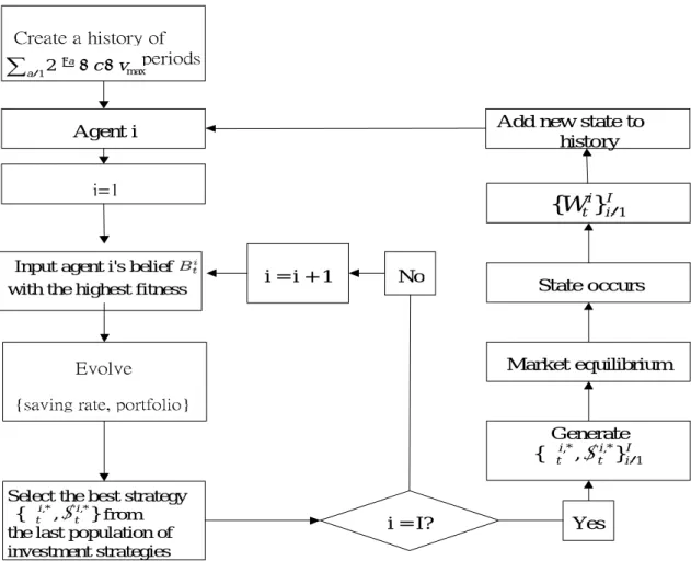
3.2 Summary

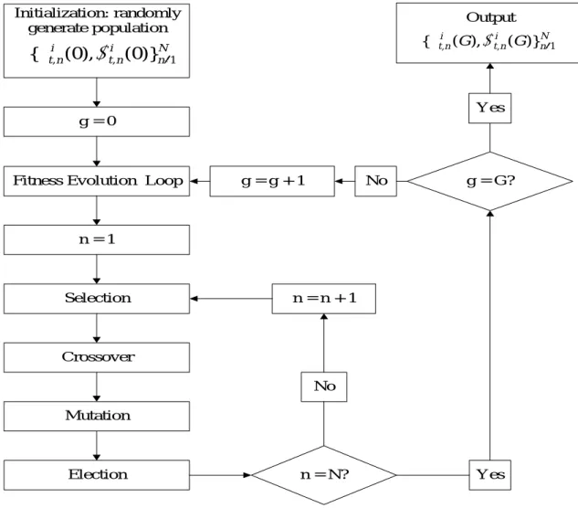
Figure 2 is a summary of the agent-based artificial stock market.

4 Experimental Designs and Data Generating Processes

Two series of experiments are conducted in this paper. Each design can be summarized by a design table, such as Table 1, which characterizes Experiment 1. Each experimental

Agent i

i=1

Input agent i's belief with the highest fitness

Market equilibrium State occurs

Generate

Select the best strategy from

the last population of investment strategies

i = I? Yes No

i = i + 1

Evolve

{saving rate, portfolio}

Add new state to history Create a history of periods max 12 c v a a_{+ +}

∑

W

}

{

Figure 2: A Summary of Agent-Based Artificial Stock Markets

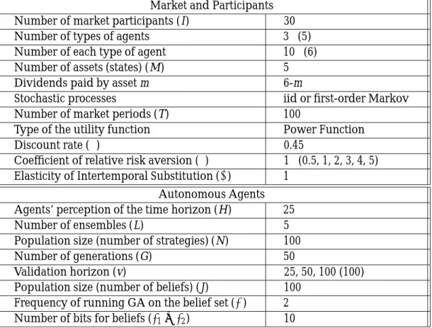
design may differ in only few parameter values, and share the same for the rest. There-fore, we can use Table 1 to state the common structure of the two experiments. The parameters used to control the experiments can be classified into two categories. Param-eters of the top half of Table 1 correspond to the market and its participants, whereas those of the bottom half pertain to the adaptive scheme (i.e. genetic algorithms) associ-ated with the autonomous agents.

To examine the influence of bounded rationality on the observed elasticity, in the first experiment, we distinguish agents by their forecasting accuracy. As what has been shown in Chen and Huang (2007a), this can be done by endowing agents with different valida-tion horizon (v).9 _{Chen and Huang (2007a) has shown that a longer validation}

hori-zon implies higher forecasting accuracy, and, other things being equal, a higher wealth share. In the first experiment, we consider agents with three different values of v, namely,

v = 25, 50, 100. These three types of agents are evenly distributed among a market of 30

participants; so there are 10 agents associated with each v (See Table 1).

Agents in the first experiment share the same utility function, i.e., the log utility func-tion, which impliesρ= ψ =1 (Table 1). The purpose of the first experiment is to examine

Table 1: Experimental Design

Market and Participants Number of market participants (I) 30 Number of types of agents 3 (5) Number of each type of agent 10 (6) Number of assets (states) (M) 5 Dividends paid by asset m 6-m

Stochastic processes iid or first-order Markov Number of market periods (T) 100

Type of the utility function Power Function

Discount rate (β) 0.45

Coefficient of relative risk aversion (ρ) 1 (0.5, 1, 2, 3, 4, 5) Elasticity of Intertemporal Substitution (ψ) 1

Autonomous Agents Agents’ perception of the time horizon (H) 25

Number of ensembles (L) 5

Population size (number of strategies) (N) 100 Number of generations (G) 50

Validation horizon (v) 25, 50, 100 (100) Population size (number of beliefs) (J) 100

Frequency of running GA on the belief set (Δ) 2 Number of bits for beliefs (τ1+ τ2) 10

Experiment I and Experiment II share the values for most parameters. For those they don’t, we put the values used in Experiment I outside the bracket, whereas leave the values used in Experiment 2 inside the bracket.

whether we can discover these coefficients by using the standard econometric procedures with the artificial data on consumption and returns.

The second experiment assumes agents to share the same perception parameter (val-idation horizon), while differs them by risk preferences. Motivated by Chen and Huang (2007b), we vary the value ofρ from 0.5, 1, 2,..., to 5, as shown in Table 1. As shown in Chen and Huang (2007b), risk aversion contributes to the wealth share in a positive way: the higher the coefficientρ, the higher the wealth share. The purpose of this experimen-tal design is then to see whether we are able to discover the true value for each of the six values ofρ or their reciprocals (ψs).

For each design of the two experiments, 100 runs are conducted, and each last for 100 periods. For the 50 out of these 100 runs, we employ iid as the state-generation mecha-nism, whereas, for the other 50 runs, the first-order Markov process is used.

4.2 Data Generated

Based on the theoretical model presented in Section 3, the simulation counterpart can generate a number of time series observations, including individual behavior and

aggre-gate outcomes. Since these variables will be then be used in the econometric analysis for the later stage, we shall first briefly summarize them here.

Let start with individual profiles. The individual behavior as described by Equations (8) to (13), and with the modifications (18) to (21), covers the following time series of individual profiles.

• {ci

t}, (i = 1, 2, ..., I): individual consumption

• {δi

t}, (i = 1, 2, ..., I): individual saving rate

• {αi

m,t}, (m = 1, 2, ..., M, and i = 1, 2, ..., I): individual portfolio

• {qi

m,t}, (m = 1, 2, ..., M, and i = 1, 2, ..., I): individual holding share of each asset

• Time series of aggregate consumption ({ct})

• Time series of asset price ({pm,t}, m = 1, 2, ..., M)

5 Econometric Analysis of the Simulation Results

5.1.1 Estimation Using the Individual Data

The main econometric equation or the system of equations which we shall built upon to estimate the parameter of EIS is mainly based on Hall (1988).10

Δci t = τi+ ψirit−1+ ξit. (i = 1, 2, ..., I), (22) where Δci t = log( ci t ci_t−1). (23)

Notice that the heterogeneity of individuals in terms of the elasticity of intertemporal substitution makes Equation (22) also heterogeneous among agents. Therefore, all esti-mated coefficients, such asτ and ψ, are heterogeneous among agents as they are denoted byτi andψi. Furthermore, the heterogeneity in terms of investment behavior also make rates of return rt facing agents also heterogeneous, which are denoted by ritin Equation

(22).

The return facing each individual is determined by their chosen portfolioαi_t, and can be calculated as follows. rti = log(Rit) (24) where Rit= M

∑

Equation (26) gives the rate of return of the asset m, and Equation (25) is the rate of return of the portfolioαi_t.11 Following the derivation of the Euler consumption equation (see Appendix C), we do not use the rate of return (Ri

t) but the logarithm of it (rit) as the

dependent variable.

To estimation coefficients ψi, one may start with Equation (22), and estimate each of

the 30 equations individually. Alternatively, one may consider the set of 30 individual equations as one giant equation, and estimate the 30ψis altogether. The latter approach is

the familiar seemingly unrelated regression estimation (SURE). SURE can be useful when the error terms (ξi

t) of each equation in (22) are related. In this case, the shock affecting the

consumption of one agent may spill over and affect the consumption of the other agents. In this case, estimating these equations as a set, using a single large equation, should improve efficiency. In this paper, we do find the error terms among different agents are correlated; therefore, SURE is applied. To do so, we rewrite the set of equations (22) into a single equation as (27). Δc = Γ + rΨ + Ξ (27) where Γ = ⎛ ⎜ ⎜ ⎜ ⎝ τ1 τ2 .. . τ30 ⎞ ⎟ ⎟ ⎟ ⎠,Δc = ⎛ ⎜ ⎜ ⎜ ⎝ Δc1 Δc2 .. . Δc30 ⎞ ⎟ ⎟ ⎟ ⎠, r= ⎛ ⎜ ⎜ ⎜ ⎝ r1 0 ... 0 0 r2 ... 0 .. . ... . .. 0 0 ... r30 ⎞ ⎟ ⎟ ⎟ ⎠,Ψ = ⎛ ⎜ ⎜ ⎜ ⎝ ψ1 ψ2 .. . ψ30 ⎞ ⎟ ⎟ ⎟ ⎠,Ξ = ⎛ ⎜ ⎜ ⎜ ⎝ ξ1 ξ2 .. . ξ30 ⎞ ⎟ ⎟ ⎟ ⎠. Here, we remove the subscript t, so eachΔci, riandξiare column vectors, which presents, respectively, the dependent, independent observations and error terms at each period t (t= 1, 2, ..., T). The ordinal least square (OLS) can not be directly applied to Equation (27) because, as we mentioned earlier, consumption residuals (ξi_t) among different agents are correlated. Furthermore, based on the White test, evidence of heteroskedasticity is also found in each of the equations (22). These evidence together indicate that one should use the generalized least squares (GLS) rather than OLS to estimate Equation (27).

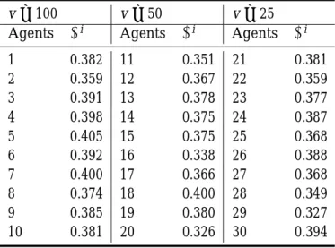
The GLS estimation of the vector Ψ is given in Table 2. The estimate ˆΨ contains the elasticity of the intertemporal substitution of 30 agents, who, under Experiment 1, differ only in the parameter validation horizon (v). In Table 2, we cluster the agents with the same validation horizon together, and number them accordingly. So, we number one two ten for the agents with the longest validation horizon (v= 100), eleven to twenty for the agents with middle validation horizon (v = 50), and twenty one to thirty for the agents with shortest validation horizon (v = 25).

While the true value of ψi _{is identically one for all agents, the estimated counterpart}

is numerically different among agents. It ranges from a minimum of 0.326 (Agent 20) to a maximum of 0.405 (Agent 5). This range is also very much below than one, and the average 0.374 is just about one-third of the true value. As a result, we fail to discover the agents’ true preference of intertemporal substitution; instead, it is dramatically underes-timated, which means, on the other hand, if we take the reciprocal of it as the estimate of the coefficient of risk aversion, then obviously, it is overestimated.

11_{The rate of return defined here (26) is not conventional. Appendix C discusses the reason of using this} one. See also footnote (16).

Table 2: The Estimated Elasticity of Intertemporal Substitution, Individuals

v= 100 v= 50 v= 25

Agents ψi Agents ψi Agents ψi 1 0.382 11 0.351 21 0.381 2 0.359 12 0.367 22 0.359 3 0.391 13 0.378 23 0.377 4 0.398 14 0.375 24 0.387 5 0.405 15 0.375 25 0.368 6 0.392 16 0.338 26 0.388 7 0.400 17 0.366 27 0.368 8 0.374 18 0.400 28 0.349 9 0.385 19 0.380 29 0.327 10 0.381 20 0.326 30 0.394

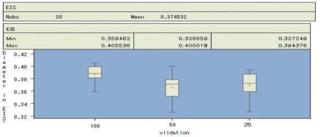
To give a further examination of the estimated EIS ( ˆψi_{) among agents with different}

perception (v), Figure 3 depicts the box-whisker plot of the ˆψi of each group. It can be seen that agents with the long validation horizon (v = 100) tends to have a higher value of ˆψi_{, while the distribution associated with the medium horizon (v = 50) and the short}

horizon (v = 25) is almost the same.

At this stage, it is still too early to infer whether our simulation results can shed light on the empirical evidence on the heterogeneity in either the risk aversions or the intertem-poral substitution, as we have seen in Section 2.2.3. However, it does question whether the observed heterogeneity, either in ψ or ρ, is just spurious, that including the empir-ically positive relation betweenψ and wealth. Having said that, we shall compare the estimatedψi of the “rich” people and that of the “poor” people by using our simulation results.

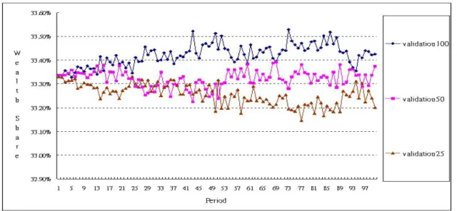
Figure 3 shows the wealth share of the three groups of agents. As Chen and Huang (2007a) already showed, the agents with a long validation horizon tends to have a higher wealth share than those with a short one, which is consistent with what we have here. In our Experiment 1, the richest group of agents (agents with v = 100) owns 0.7% more in share than the poorest group of agents (agents with v = 25), and the “middle class” (agents with v= 50) owns 0.4% less than the richest ones, but 0.3% more than the poorest ones. These differences are numerically slight, but are statistically significant. Combin-ing this result with that of Figure 3, we find that the richest group of agents is also the one with the highest ˆψ. However, from our setting, these agents, be they eventually poor or rich, share the same EIS, which is one. As a result, the observed heterogeneity may be spurious. Alternatively speaking, in our agent-based simulation, both the wealth share and the observed relation between consumption and the return are endgeneously gen-erated. Agents with a better forecasting accuracy may be able to behave closer to the optimizing behavior (Euler consumption equation); hence, they are not only richer but their observed EIS, ˆψi, is also closer to the true value.

Figure 3: The Estimated EIS ( ˆψi) of Agents with Different Perception (Validation Hori-zons)

5.1.2 Estimation Using the Aggregate Data

As we survey in Section 2.1, the early econometric work on the estimation of the elasticity of intertemporal substitution mainly used only the aggregate data. The result which we have in the previous section (Section 5.1.1), however, use the individual data instead. Therefore, to conduct experiments in parallel to the early work and to examine the effect of aggregation upon the estimation of the EIS, in this section, we also estimate the EIS based on the aggregate data.

The data generated by the agent-based simulation is flexible enough to allow for dif-ferent levels of aggregation. We consider two difdif-ferent levels of aggregation. At the first level, we employ the device of the representative agent for each group of agents, i.e., agents with the same validation horizon. We then derive the consumption and return data for this representative agent, and estimate the Euler consumption Equation based on the derived (aggregated) data. At the second level, we then consider the whole econ-omy as a unit, and repeat the same thing above with the device of the single represent agent. This will lead to the two following modifications of Equation (27), namely, Equa-tions (28) and (31). Δc = Γ + rΨ + Ξ (28) where Γ = ⎛ ⎜ ⎝ τL τM τS ⎞ ⎟ ⎠ , Δc = ⎛ ⎜ ⎝ ΔcL ΔcM ΔcS ⎞ ⎟ ⎠ , r = ⎛ ⎜ ⎝ rL _{0 0} 0 rM 0 0 0 rS ⎞ ⎟ ⎠ , Ψ = ⎛ ⎜ ⎝ ψL ψM ψS ⎞ ⎟ ⎠ , Ξ = ⎛ ⎜ ⎝ ξL ξM ξS ⎞ ⎟ ⎠ ,

Figure 4: Wealth Share of the Three Groups of Agents and ΔcL t = log( ∑ 10 i=1cit ∑10 i=1cit−1 ), ΔcM t = log( ∑ 20 i=11cit ∑20 i=11cit−1 ), ΔcS t = log( ∑ 30 i=21cit ∑30 i=21cit−1 ), (29) rL = log( ∑ 10 i=1Rit 10 ), r M _{= log( ∑}20i=11Rit 10 ), r S_{= log( ∑}30i=21Rit 10 ), (30)

Equation (28) is the Euler consumption equation with the assumption of treating each group of individuals as a single representative agent. Equation (29) is the growth rate of the group consumption, and the group consumption is simply defined as the sum of the individual consumption. Equation (30) is the logarithm of the return facing each representative agent, and this return is defined as the simple average of the returns facing each individuals of the group. The superscripts L, M, and S refer to the long, medium and short validation horizons. As what we did in Equation (27), the subscript t is not shown here, since each of the three-group components inΔc, r and Ξ are considered as column vectors composed of time series observations.

Likewise, Equation (31) is the Euler consumption equation with the assumption of treating the whole economy as a single representative agent. This version is the one fre-quently used in macroeconometrics. Equations (32) and (33) are the further aggregation in parallel with Equations (29) and (30).

Δct = τ + ψrt−1+ ξt, (31) where Δct = log( ∑ 30 i=1cit ∑30 i=1cit−1 ), (32) and rt= log( ∑ 30 i=1Rit 30 ). (33)

Table 3: The Estimated Elasticity of Intertemporal Substitution, Groups

Aggregation Level I: Equation (28)

Parameter Estimate Std Err t Value Pr> |t| R2 ˆ ψL _{0.05427 0.0017 31.99 <.0001 0.0925} ˆ ψM _{0.05388 0.0017 31.31 <.0001 0.0895} ˆ ψS _{0.02829 0.0011 25.07 <.0001 0.0013}

Aggregation Level II: Equation (31)

Parameter Estimate Std Err t Value Pr> |t| R2 ˆ

ψ 0.08678 0.0024 35.06 <.0001 0.1115

SURE with GLS is then applied to the aggregate Euler consumption equation (28), whereas GLS alone is applied to Equation (31). The estimation results are presented in Table 3. The estimated EIS of the three groups of agents, ˆψL_{, ˆψ}M_{, and ˆψ}S_{, are given in the}

upper panel of Table 3, whereas the economy-wide counterpart, ˆψ, are given in the lower panel. These estimates are in a sharp contrast to the those estimates based on individual data (see Table 2). In Table 2, we have seen that the EIS has been underestimated, and the estimate is about one-third of the true value. However, here it is further underestimated and is even less than one-tenth of the true value.

Among the three groups of agents, agents with better forecasting accuracy (longer validation horizons) are still found to be ones with higher estimated EIS: ˆψL > ˆψM >

ˆ

ψS_{. In particular, for the agents with short validation horizon, the estimated EIS is only}

0.028, and the respective R2_{is barely above zero. Therefore, the general findings of using}

individual data sustains, namely, the observed heterogeneity in the EIS is spurious. So is the observed positive relation between wealth share and the EIS.

One interesting question frequently asked in the agent-based modeling is: what is the relation between micro and macro. By comparing the ˆψ from the aggregate data (Table 3) and the ˆψiof the individual data (Table 2), one may find that the representative agent of the whole economy constructed using the aggregate data does not well represent the distribution of individuals. An ˆψ of 0.086 is far below the entire the distribution of ˆψis,

not to mention being the mean or median of it. 5.2 Experiment 2

5.2.1 Estimation Using the Individual Data

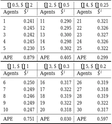
The second experiment assumes agents to differ in risk preference. While all of them have the CRRA-type risk preference, theirρs are different and range from 0.5, 1, 2,..., to 5. Five agents correspond to each of the six values ofρ. We number these agents from 1 to 30 by the value ofρ as shown in Table 4. As before (27), SURE is applied to estimate the intertemporal elasticity of each agent, and the results are given in Table 4.

Table 4: The Estimated Elasticity of Intertemporal Substitution (Experiment 2), Individu-als

ρ = 0.5, ψ = 2 ρ = 2, ψ = 0.5 ρ = 4, ψ = 0.25

Agents ψˆi Agents ψˆi Agents ψˆi 1 0.241 11 0.290 21 0.321 2 0.245 12 0.295 22 0.326 3 0.242 13 0.300 23 0.327 4 0.245 14 0.298 24 0.326 5 0.230 15 0.302 25 0.322 APE 0.879 APE 0.405 APE 0.299

ρ = 1, ψ = 1 ρ = 3, ψ = 0.3 ρ = 5, ψ = 0.2

Agents ψˆi Agents ψˆi Agents ψˆi 6 0.250 16 0.317 26 0.319 7 0.249 17 0.322 27 0.318 8 0.246 18 0.319 28 0.319 9 0.249 19 0.322 29 0.322 10 0.247 20 0.318 30 0.317 APE 0.751 APE 0.030 APE 0.597

Table 4 presents the estimated elasticity of the six groups of agents; each is associated with different ρ (ψ). Since the utility function is the CRRA type, the true ψ is just the reciprocal of the correspondingρ. In Table 4, we also list the value of the ψ in parallel. This makes us easier to compare ˆψiwithψi.

From Table 4, a few observations can be made. Firstly, while ψs vary from 0.2 to 2, their estimated counterparts distribute within a much narrower range, namely, around 0.25 to 0.3. With this range, most of the estimated ψs miss their true values. The ψ of less risk-averse agents are underestimated, whereas theψ of more risk-averse agents are overestimated. To see this, the average percentage error (APE) of eachψ are also given in Table 4. It is clear that, starting from the less risk-averse agents (ρ=0.5), the APR starts to decline, and further down to the minimum whenρ approaches 3. It then increases again whenρ is away from 0.3. Second, associated with this APE pattern, there is a positive relation between the ˆψi and ρ. If the positive relation between the wealth share and ρ still exists as in Chen and Huang (2007b), then we have found again a positive observed relation between wealth share and estimated intertemporal elasticity.

5.2.2 Estimation Using the Aggregate Data

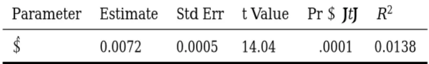
In vein of Section 5.1.2, we also examine an aggregate version of the Euler consumption equation, which in structure is very similar to Equation (31). Due to the very usual econo-metric consideration, generalized method of moment is applied to estimate the aggregate

Table 5: The Estimated Elasticity of Intertemporal Substitution, Groups

Parameter Estimate Std Err t Value Pr> |t| R2 ˆ

ψ 0.0072 0.0005 14.04 <.0001 0.0138

Euler consumption equation, and the result is shown is Table 5. By comparing this result with the previous one (Table 5). One can see the sharp decline of the estimated intertem-poral elasticity. Remember that we have agents with elasticities from 0.2 to 2; however, the estimated elasticity is almost nil, while still significantly different from zero. There-fore, the representative agent does not represent the society at all: it is not the centroid (average) of them.

Also, by comparing this result with the that from the earlier aggregate Euler consump-tion equaconsump-tion (Table 3), one may gauge the possible implicaconsump-tion of the degree of hetero-geneity on the estimated elasticity. In the early case (Experiment 1) all agents share the same degree of risk aversion, and now they are divided into six groups of risk aversions. The ˆψ decreases from the early 0.0867 to now only 0.0072, and R2 also drops from the original 11.15% to now only 1.38%. Therefore, by using aggregate data, the intertempo-ral elasticity may be further underestimated when agents’ risk preference are heteroge-neous.12

6 Concluding Remarks

One of the main attractions of using the agent-based model is its capability to demon-strate the so called micro-macro relation. Sometimes, it may not be easy to track, step by step, from the bottom (micro interactions) to the top (macro outcomes), and hence one may not be able to have a full grasp of the causes and the consequences. Nevertheless, it does allow us to gauge how serious a misleading conclusion one may draw when the analysis is entirely based on the aggregate outcomes. In this paper, an illustration based on the famous elasticity puzzle is demonstrated.

Our results based on the agent-based simulation show that the puzzle may come from our ignorance of a fundamental issue: can we use econometrics to discover the individuals’

profiles while they are boundedly rational and are placed in an interacting and evolving environ-ment. Both of the two experiments show that the intertemporal elasticity of individuals

are underestimated, and the degree of underestimation is even severe when only aggre-gate data is used. Furthermore, we also find that agents who have better forecasting capability and hence wealthier tend to have a higher “observable” intertemporal elas-ticity than those with less forecasting accuracy, even though they both share the same intertemporal elasticity. Therefore, the observed positive relation between wealth share and the intertemporal elasticity can be spurious.

There are a number of points which are open for further research. First of all, the robustness of some of the results observed in this paper should be further examined by

using different econometric procedures. In this paper, we do not use OLS because of the econometric reason. However, we have found that if one uses OLS, the already under-estimated intertemporal elasticity (found in Experiment 1) can be even biased away, and the results can nicely match many empirical results, such as Hall (1988) and Campbell (2003).

Second, the independent variable, return, only considers dividends. The capital gain is not included for the reason that given in the appendix. However, it is still interesting to see the results by “blindly” trying the version with capital gains. Third, all individual knows their own returns, while this personal data is not easy to get in empirical study. So, it would be also interesting to see the relation between consumption and return, when the latter is defined by only the observable market data.

Appendix A Evolution at the Low Level: Investment Strategies

The implementation of the genetic algorithm starts with a representation (coding) of so-lutions. Here, we employ the real coding. The saving rate (δit) and the portfolio (αit) are

coded as real-valued numbers: {δ_ti | αi_1,t,αi_2,t, ...,αi_M,t}. To solve (18), an initial popula-tion of investment strategies with populapopula-tion size N is first generated for each investor i,

GEN_t,0i ≡ {δit,n(0), αit,n(0)}Nn=1. The number inside the parentheses refers to the generation

number in the GA cycle. Population GENi

t,0is generated as follows:

• δi

t,n(0) is randomly generated from the uniform distribution U(0, 1).

• To generate a portfolio αi

t,n(0), a set of numbers (Q1, Q2, ..., QM) are randomly

gen-erated from U(0, 1). Then, to make sure that their sum is equal to 1, they are rescaled as follows: ( Q1 ∑M q=1Qq , Q2 ∑M q=1Qq , ..., QM ∑M q=1Qq ). (34)

Appendix A.2 Fitness Evaluation: Eval{ GEN_t,gi }

Corresponding to (18), the fitness measure f is simply the H-horizon discounted expected utility: ft(n, g) ≡ f (δt,ni (g), αit,n(g)) ≡ E{ H−1

∑

where ft(n, g) refers to the fitness of the nth investment strategy in the population GENt,gi

(i.e. the gth generation of the GA cycle). The Monte Carlo simulation technique is used to evaluate the fitness (35). The way to do so is to simulate a certain number, say L, of

H-horizon histories of the states based on investor i’s belief, B_ti. For each simulated history

l (l ∈ [1, L]), we can obtain a realization of (35), i.e.

H−1

∑

h=0

(βi₎h_ui_(ci

Then, we estimate ft(n, g) by taking the sample average,

ˆft(n, g) = ∑ L

l=1∑hH−1=0(βi)hUi(cit+h| l)

L . (36)

Appendix A.3 Genetic Operation: GEN_t,gi → GEN_t,gi ₊₁

Once the procedure Eval{ GENt,gi } is completed, all investment strategies are associated

with a fitness which is the output of (36).

Eval: {δt,ni (g), αit,n(g)}Nn=1→ { ft(n, g)}Nn=1 (37)

Based on their fitness, we shall revise and renew these investment strategies based on investor i’s belief Bi_t. This revision and renewal procedure involves the use of four standard genetic operators, namely, selection, crossover, mutation and election.

Selection: The tournament selection with tournament size 4 is employed. For each se-lection, four investment strategies are randomly selected from GEN_t,gi . Of them, the best two will be chosen as the parents (mating pool). We denote them by Ix ≡ {δt,xi (g), αit,x(g)},

and Iy≡ {δit,y(g), αit,y(g)}, where x, y ∈ [1, N].

Crossover: With probability pcross (crossover rate), the two parents chosen above will

generate an offspring by taking a weighted average of the two investment strategies, and the weights will be determined by the relative fitness of the two strategies.

Iz ≡ (δit,z(g), αit,z(g)) (38) = ft(x, g) ft(x, g) + ft(y, g)(δ i t,x(g), αit,x(g)) + ft(y, g) ft(x, g) + ft(y, g)(δ i t,y(g), αit,y(g))

Mutation:The offspring Izwill then have a small probability (mutation rate) to mutate.

If mutation happens, it will proceed as follows. For the saving rate, a number randomly selected from the U[0, 1] will be used to replace δi

t,z(g). For the portfolio, a set of

num-bers, ≡ (1,2, ...,M), randomly generated from U(0, 1), will replace αit,z(g). Then the

rescaling technique described in (34) will be applied. We call the resultant strategy Iz .

Election:The use of the election operator examines whether the new investment strat-egy is expected to perform better than the one it replaced. In election, we shall use (36) to evaluate the potential fitness of Iz , and compare it with the fitness of the two parents, Ix

and Iy. Then, only the one with the highest fitness will be retained for the next generation,

GENi t,g+1.

Appendix A.4 Loops

Once a new investment strategy is generated, a loop leads us back to selection, which is then followed by crossover, mutation and election and then the next new investment strategy is generated. The loop will continue until all N strategies of GEN_t,gi ₊₁are gener-ated. GENi

t,g+1will be evaluated based on the Eval procedure, and based on the

evalua-tion, genetic operators will be applied to GEN_t,gi ₊₁to generate GEN_t,gi ₊₂. This loop will also be repeated over and over again until a termination criterion is met, e.g., when g reaches a prespecified number G.