A new design of adaptive robust fuzzy controller for nonlinear systems

(1)

PmwJlnps of lhc

Armdm Contml Conhnnce

SoaHIe, Washington Juno 19H

FA12

-

10:35

A

New Design

of Adaptive Robust Fuzzy Controller for Nonlinear

Systems

Feng-Yih Hsul and Li-Chen Fu1,2

Dept. of Electrical Engineering'

Dept. of Computer Science & Information Engineering2

National Taiwan University, Taipei, Taiwan, R.O.C.

Abstract

This paper presents an adaptive robust fuzzy control architecture for a class of nonlinear dynamic systems which are either ill-defined or rather complex. The control objective is to adaptively compensate for the unknown plant nonlinearity, which is represented as a fuzzy rule-base con- sisting of a collection of if-then rules. The algorithm embedded in the proposed architecture can automatically update fuzzy rules and, consequently, is guaranteed to be globally stable and to drive the tracking errors to a neigh- borhood of zero. Focused on realization, hardware limitations such as traditional long computation time and excessive memory-space usage are also relaxed by incorporating heuristic concepts, which reveals the flexible feature of this architecture. Simulations are run for the control of a sim- plified circuit system, and results show that the proposed control architecture is featured in fast convergence.

1 Introduction

During the past decade, intelligent control methodologies have gradually been recommended to solve a number of complicated problems that, especially, conventional control methodologies are hard to handle. Those methodologies often use biologically motivated techniques and pro- cesses, and are referred to as neural networks, fuzzy-de base, knowledge-base, or other learning schemes. Unlike general conventional schemes based on a complete theory and algorithmic structure, they are in general hardly evaluated. Therefore, it is imperative to make efforts on

bridging the gap between the conventional control scheme and the intelligent ones [I]. Recently, analysis on intelligent control has attracted enormous research interests [2]- [SI. Ideas behind those schemes are to strengthen their

theoretic basis but at the price of expensive implementation by using massive networks and extensive rule-tables or complex functions, which generally lead to difficulties in real implementation due to hardware limitations such

as long computation time and excessive memory-space usage.

On

the other hand, the heuristic nature of intelligent control often has substantial benefit for a controlled system. Hence, an integrated consideration is suggested in this paper.

In this paper, we present a new fumy control method- ology which can be applied to the control of a class of nonlinear systems. It is known that fuzzy logic controllers (FLC) have been widely applied in industry. An important advantages of using FLC is that fuzzy theories can capture

the approximate, qualitative aspects of human knowledge and reasoning. Apparently, such control provides a rather feasible alternative for a plant that is complex or ill-defined

[IO]. To extend the range of application of FLC, the cur-

rent research efforts have been made as how to automatically generate rules or how to adaptively update the existing rules. There is a common feature in those proposed

schemes, namely, the fuzzy theory is always combined with

some other control architectures such as neural networks

[lo], [ll], adaptive control [8], learning control [9], etc.

Particularly, adaptive control concept is often incorporated into some other intelligent schemes. For examples, Mess- ner et al. in [7] proposed a new adaptive learning scheme which uses some kernel function of time as a general re- gressor. Contrarily, in [2], a spatial Fourier transform is adopted to furnish a more general kernel function of state which is then realized by a Gaussian radial network. But unlike the two, the fuzzy basis function is assumed in [8]

with a viewpoint that a heuristic algorithm used for control tends to be more flexible in satisfying the approximation need. Apart from the above adaptive concept, another robust control concept also has to be adopted to ensure that the overall controlled system is stable. Thus, a control synthesis is proposed here, which combines the adaptive fuzzy control approach and a robust control approach to generate the final adaptive robust fuzzy control (ARFC) scheme.

2

Problem Formulation

Consider a class of nonlinear systems described by the following dynamic equations expressed in canonical form:

P ( t ) = f(z(t), k ( t ) , P ) ( t ) ,

.

* *

,

z'"-"(t))

+

b ( z ( t ) , k(t),z'"(t),

.

* ,z'"--l'(t))u(t), ₍₁₎

where u ( t ) is the scalar control input, f is an unknown function, and b is an unknown positive control gain such

that b

2

S with 6

>

0. Our control objective is to track a desired trajectory, i.e., to force the plant state (vector) x = [z, k,

d2),

...,

z ( " - ' ) ] ~ to follow a specified

desired trajectory = [zd,

&,

zp),

...,

SF-^)]^.

After defining the tracking error (vector) e = x d ( t )

-

x ( t ) =

[e,e, e@),

...,

e(n-l)]T, our goal is thus to design a control

u ( t ) which ensures that e ( t )

-+

0 as t

+

00.

Generally, the controller design will require the knowledge of

f

and b to some degree of accuracy. But for more

(2)

complex or ill-defined systems, f and b can not be e=-

ily estimated well, which will then result in uncertainties in plant modeling. Commonly speaking, the uncertainties are often denoted as a deviation of the actual plant from the nominal plant. Let F =

-b-'f

and 3 = b-',then the uncertaintks are den_oted b L A F = -b-'f

-

F and A B = b-'

-

B, where F and B are nominal version of

-b-'f and b - l , respectively. Given this nominal plant

subject to the foregoing control objective, a nominal controller

D

is designed as follows:

(2)

A

u = ~ + ~ x l . + k s s ,

where s is a sliding mode variable s = Xoe

+

A11

+

...

+

e("-') = [Xo,Al,

...,

1ITe = XTe with the transfer function A b ) = p"-'

+

An-2pn-2

+.

. .

+

Alp

+

A0 being a Hurwitz polynomial, and ks

>

0, xr = zg)+Xoe+-. -+X,-2ef"-1).

If we let the real control be U =

+

Au, where Au is to be specified later, then the dynamic equation of the sliding mode variable s is given as:

b-'i = - k s ~ f A F

+

AB%,

-

Au. ₍₃₎ Apparently, in addition to the nominal controller mentioned above, the system will need an extra control term, namely, Au to compensate for the existing uncertainties. Since A F and A 3 are not available, from a p r e c a l s t g - point, A F and A B will be approximated by A F and AB, respectively, as closely as possible. With this observation in mind, a general nonlinear compensation function extra to the nominal control is devised as follows:

Au = Uf 4- u b 4- U S . ₍₄₎

h -cI

where u f , u b , us are given as uf = AF, U b = AB%,, and

us = U(x,x,)sgn(s). Assume that luf

-

AFI

5

E ~ ( x ) ,

1ub

-

ABxrI

5

q ( X , z,), and

u(x,

2,)

2

Ef

+

Eb, then the t_racking_errors will asymptotically converge to zero. Since

F and B are hard to be approximated by using conventional control schemes, some intelligent control concepts need to be adopted. Moreover, since us is not continuous, undesirable chattering may appear due to excessive mag- nitude design of u s , which therefore require a suitable us not only ensuring the system robustness but also the per- formance of the controlled system. Consequently, in this paper, an ARFC is proposed to perform exactly as such

an intelligent nonlinear controller.

3 Control Algorithm

In

this section, the

ARFC

will be introduced.

3.1 f i z z y Knowledge Representation

n o m a practical point of view, a complex or ill-defined system is always represented by variables which are as-

sociated with some physical meanings such as the Mach number, the angle-of-attack in a flight system, or voltage, current in a circuit system. Hence, the system originally described by (1) may be represented as follows:

zfn) = f(zfx (z,

. .

* ,z(,-I)),

.

* .

,

Zfi (2,.

. .

, z + q , .

. .

,

Zfnf(X,*",z("-'))) + b ( Z b ~ ( x , " ' , 2 ( n - ' ) ) , . ' . ,

Zbj (S, * *

,

x(n-')), '

.

',

z b n b (x, ' '

.

,z'n-l'))U(t), _{( 5 )}

dimensions of z f and Z b , respectively. Given this notion,

a fuzzy rule-based system is built.

As a general description of fuzzy knowledge representation

[$I,

a fuzzy rule-base consists of a family of fuzzy

an input linguistic vector in the discourse universe

U.

and

L, =

{ L ~ , L ~ , . . . , L ~ ' , . . . , L ~ ~ ~

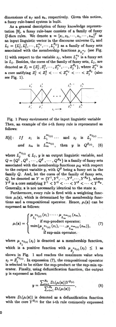
as afamily of fuzzy sets associated with the membership functions fiL:j (see Fig.

1) with respect to the variable zj, where

Lj"'

is a fuzzy set in

Lj.

Besides, the cores of the family of fuzzy sets, Lj

,

are denotedas

Zj

= ( Z j l , Z j 2 , . . . , Z j a j , . . . , Z ~ } , where 2;' is

a core satifying

Z;

<

2;

< . .

.

<

zjfj

< . . <

Z? (also

see Fig. 1 ) .

If-then rules. We denote z

=

[a,

z2,

.

-

.

,

zi

,

.

,ZmIT as

R .

3

r : L:

Fig. 1 Fuzzy enviroment of the input linguistic variable Then, an example of the i-th fuzzy rule is represented as

follows:

and zm is L:"('), then y is

QB('),

(6) where

LT(')

E

Lj,

y is an output linguistic variable, and

Q = {Q'

,

Q 2

,

.

,

Q R v } is afamily of fuzzy sets associated with the membership functions p~ with respect to the output variable y, with

Q p

being a fuzzy set in the family

Q.

And, let the cores of the family of fuzzy sets,

Q,

be denoted as Y = { Y ' , Y 2 , . . . , Y p , . . . , Y R Y ) , where

Y @ is acore satisfying Y'

<

y 2

<

Y @

<

y R v .

Generally, z is not necessarily identical to the state x.

Furthermore, every rule is fired with a weighting function p ; ( z ) , which is determined by the membership functions and a compositional operator. Hence, pi(.) can be expressed as follows:

,

QB

,

PL;l(i) k 1 ) * * *

-

PL;m,mfi) (zm),

min{PLPl(i) (a), * .

,

PLZ"(i) (zm)), (7)

if sup-product operator; if sup-min operator

L

p ; ( z ) =

where p aj(il (Zj) is denoted as a membership function,

which is a positive function with p ~ j ( ~ ) (Zj)

5

1 as

shown in Fig. 1 and reaches the maximum value when qj =

Zj

'('I. In expression (?), the compositional operator

is selected to be either the supproduct or the shpmin operator. Finally, using defuzzification function, the output 9 is expressed as follows:

L.

Z?

Q '

where zfi and Z b j are variables of the system, a =

1 , 2 , . . - , n f and = 1 , 2 , . . . , n b , with nf, n b being the

where Di(pi(z)) is denoted as a defuzzification function with the core

Yo(;)

for the i-th rule commonly expressed

(3)

as follows:

pi(.), if center-average-defuzzifier;

J-:

pQtqi)

(YPY

-

J ; I . ~ ~ O ( ~ )

(Y)

-

P ~ ( ~ ) P Y ,

Di(Pi(z))

=

if center-of-area defuzzifier;

(9)

{

where y-* and y* are solution values of y satisfying pi@) = pQpli) (y) with y*

2

y-* given the values z and Rt is the total number of rules generally equal to RI x R2 x x

IL.

Then, we denote a fuzzy basis function [j(z) expressed as

so that equation (8) can be rewritten as:

Rt

y = YP‘i)&(z) = @ T [ ( Z ) , (11)

i = l

where 0 = I y P ( l ) , Y P ( z ) ,

. . .

,

YP(Rt)lT is regarded as a parameter vector and [ = [&, [ 2 , .

. .

,

,$&IT

is regarded as a

regressor vector. Apparently, when Rt is large, the compu-

tation time and memory-space usage must be considered in real implementation.

As a result, we focus our attentions on computation time first, then the domain set of the fired rules and that of the total rules should be clearly distinguished. First, collect the indices of the fired rules as the following set:

I = { i : Pi(Z>

>

O } , ₍₁₂₎

where pi(z) is the weighting function of the i-th &ed rules. Our aim is to figure out that the number of I, # n ( I ) , is

less than the number of total rule Rt during firing the fuzzy rules along with the expression (8) satisfied.

At the beginning, define the domain set of the total rules with respect to 1; as

Therefore, if z falls into E, then the fuzzy rules are fired to compensate the unknown functions. Partition this domain set into the finite m

-

cells, which are defined as

where a = a1 x

.

x aj x

-

. .

x a, is a product index and satisfies

2,

E

2,

ZJaj

<

ZRj.

To

union the all collection of E,, we can obtain E =

bzDEz

E,.

A 6

-

box is defined as an equivalent of E,,

n,(za,6(z)) = (2 : zJ:j

5

z j

5

ZJ?j +Sj(Z)},

= E,

where j = 1,

-

,

m , 6(z) E RmX1 and the j-th element

of 6(z) is defined as 6j(z) = ZJ:j+l

-

ZJ:’. Define the set

of all corner points of &box R, as P, = {ZCfs) : c ( z ) E

nTx1{aj,aj

+

1)). Hence the number of

Pa,

#n(P,) is

equal to 2m.

Consider the membership function (Fig. 1): 1, as zj = ~ a ’ ; 3 pL:j (Zj) = 0, as zj

2

zJ:j+l or zj

5 2P-l;

3 x p , zj”’ E (0, l), otherwise, (13)

{

for aj = 1,2,

- -

e , Rj and j = 1,2, *

.

,

m, then the following

proposition is given:

Proposition 1 If the membership functions are given as

eq. (12) and z is the linguistic vector, z E E , then ex-

ists a 6-box,

R,(Zn,G(z))

such that z E

R,(Za,S(z)),

and

# n ( I )

5

#n(P,), where # n ( I ) and #n(P,) are the num-

ber of $red fuzzy rules and that of corner points of &-box,

respectively.

Hence, the computation time is drastically reduced, especially,

as

Rt is very large.

3.2 Adaptive Robust Fuzzy Control

Referring to section 2, we use dynamical equation (5) to replace equation (1) so that a conventional control law is straightforwardly given as follows:

u ( t ) = z + + f + ? d b + u s , (14)

where 2, u f , ub, us are defined as in section 2 and here expressed in A terms of the A suggested knowledgezpresenta-

tiOn as CI = F ( Z b , z f )

+

B(Zb)$r

+

has, U f = AF(Zb,Zf),

ub = AB(Zb)Er, Us = I U s ( z b , z f , X r ) l S g n ( S ) = (U;1

+

Ixrl)sgn(s), with u : ~ , u : ~

>

0. Note that ARFC is

designed to approximate u f , U b , us, as shown in Fig. 2, by first letting F ( z F ) = - b - ’ ( z b ) f ( z f ) where ZF is given as

Z F =

[zF

zTlT, and zs = [z: sJT.

R u l e T a b l e

Fig. 2 The architecture of ARFC

Then, denote the input linguistic vectors as Z b , Z F , zs and

define the cores of the families of the fuzzy sets associated with z b , Z F and zs, respectively, as follows:

1 2 Rb

z b j = { z b j , z b j 7 9 z b j

’

}, for j = 1, 2,

..

’ nb

1 2 R..

z a j = {

zsj,

Zsj

,

. . .

,

Zsj

’

}, for j = 1,2,

-

.

-

,

ns

where n F = nb + n f

,

and ns = nF

+

1, whereby the control law can now be formally established as follows:

m F Uf =

eF

=

oFitFi(zF)

=

o%(zF);

(15) i=l mb u b = 8bxr = @bi[bi(zb)xr = @ ~ < b ( z b ) % c , ; (16) i=l ma

U6 =

eel

+

e62

I ~ ~ I

=

C(eali

+

0 ~ 2Ixrl)[si ~ (zs)

= @:iSs(zs)

+

Q , T , [ a ( z s )

Iz.1,

(17)

i=l

where O F , o b , eS1, es2 are denoted as output variables, O F ,

@a, Qsl, OS2 are denoted as parameter vectors, [ F , [a,

are denoted as regressor vectors as in equation ( l l ) , and

m F , mb, ma are denoted as the total number of rules for u f , ‘tu,, and us, respectively. Our goal is to design optimal parameter vectors and regressor vectors such that the

(4)

controlled system has minimal tracking errors and robust features. First of all, we must prove that bounds on the optimal approximation errors actually depend on the ARFC design, since that optimal parameter vectors are defined as

follows:

S>

= arg ~ ~ ~ [ S U P S F E E F ~ O % F ( Z P )

-

AFI]

= _QF'p_{m b 2 [ S U p s b ~ E b}_{l @ F & ( z b ) z r}

_-

_ABzr

I]

o:,

= arg mdn[sups,EE,0:lSe (z,)sgn(s)

I

&I

Q:2 = arg m i n [ S u p . , E E . E 3 ~ ~ , ( z s ) S g l Z ( S ) l Zr l

2

U12 1Zr11

where EF, E b and Ea are are expressed as follows:

To

simplify the problem, some mild assumptions are given as AB(@,), A F ( z F ) E C'(continuous1y differentiable),

I

AF(ZF)

I<

F U ( z ~ ) ,

I

AB(%)

I<

B u ( z b ) and

I

15 &,

where

&,

is a constant. Based on the above assump

tions, the following proposition will derive some useful re-

sults to be used in the sequel.

Proposition 2

If

the linguistic vectors Z F and z b fall into

the 6-6oxe5, s ~ ~ ( z ~ , ~ J F ( z F ) ) and n a ( . @ , t J b ( z a ) ) , respec-

tiuelg, then the optimal approximation e m r s E F ( Z F ) and

€ & i f , ) will be bounded as follows: IEFI I g F ( z F > * 6 F ( z p ) ,

their elements are defined as Q F ( = supsFEn,

[I&[]

for i

=

l , * - * , n F l g b j = sup=bmB

[I+II

for j =

1, * *

-

,nb,

Based on Proposition 2, the approximation errors can be reduced by adjusting 6~ and 6 b , and, hence, the robust controller U, with a high gain is not necessary in

ARFC.

Furthermore, let the control law be redesigned as

IcbI

5

g b ( z b ) T & b ( z $ , where W ( Z F ) = AF

-

@>*SF and

eh(!&) = AB

-

0;

( 6 ; g F ( Z F ) E

RnF,

g b ( Z b ) E pb und

O A F z

B A 3 z

U = d(t)(uf+ua+U,)+(l-d(t))U(zF, Z r ) S g n ( S ) + G , (18)

where

where a, b are some constants and a

5

;::2

5

0

5

Given the above result, we axe now ready to state the closed-loop properties of the system (5) subject to our proposed ARFC in the following theorem.

Theorem 1

If

the control law and the update law are given as in equation (18) and as in equations (21)-(24), re- spectively, then the tracking errors will asymptotically con- verge to a neigh&orhood of zero.

3.3 Two-Stage Design

From the analysis in subsection 3.2

,

it is clear that the ultimate tracking errors depend on the ranges of the deadzone, and our objective is either to raise higher precision or to reduce the total number of rules. Hence, in addition to the optimal parameter vectors, optimal regressor vectors also need to be considered. Therefore, the choice of appropriate membership functions is essential for fuzzy controller design. Here we will choose the cores of fuzzy

sets. In general, the cores of the relevant fuzzy sets are formed in two ways: (1) to use a data table; (2) via the form of function. For the former, the data set has to be memorized, which, however, requires extra memory-space.

It even costs more computation time to find the irrelevant addresses of rules. Contrarily, the latter does not face the previous difficulties, and seems to be very hard in finding a

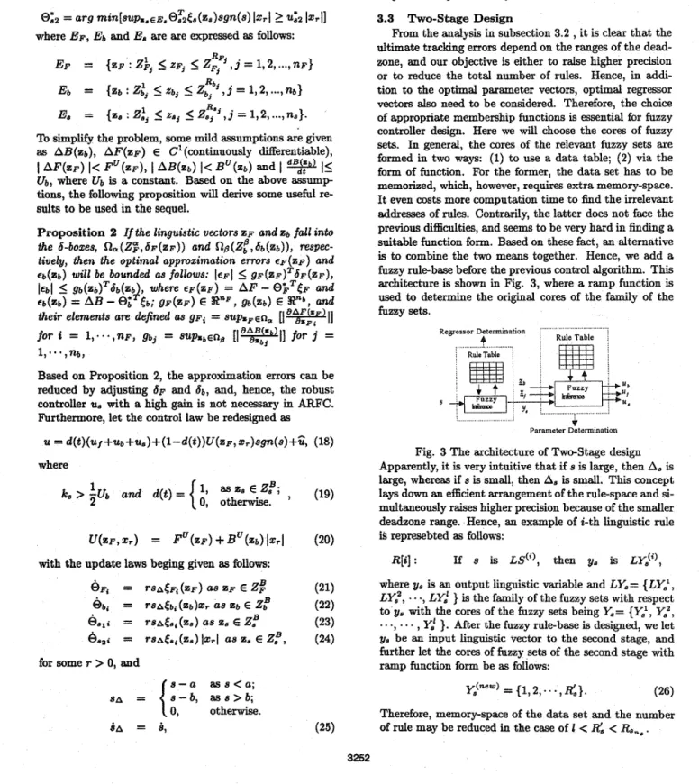
suitable function form. Based on these fact, an alternative is to combine the two means together. Hence, we add a fuzzy rule-base before the previous control algorithm. This architecture is shown in Fig. 3, where a ramp function is used to determine the original cores of the family of the

5

b. fumy sets. Regressor Determinabon A Rule Table 4 'b zb z/ 4 U/ s

+TIy

us V Parameter Determination

Fig. 3 The architecture of Two-Stage design Apparently, it is very intuitive that i f s is large, then A, is large, whereas i f s is small, then A, is small. This concept lays down an efficient arrangement of the rule-space and si- multaneously raises higher precision because of the smaller deadzone range. Hence, an example of i-th linguistic rule is represebted as follows:

R[i] : I f s is LSf'), then y, is LY,(i),

where

v,

is an output linguistic variable and LY,= {LY,l,

LK',

.

-

.,

Ay,' } is the family of the fuzzy sets with respect to pa with the cores of the fuzzy sets being

Y,=

{Y:,

Y,",

us

be an input linguistic vector to the second stage, and further let the cores of fuzzy sets of the second stage with ramp function form be as follows:

...

,

...

,

Y

.

'

}. After the fuzzy rule-base is designed, we let

y,fnew) = {1,2,.

.

,

RL}. (26)

Therefore, memory-space of the data set and the number of rule may be reduced in the case of I

<

Ri

c

Rand.

(5)

3.4 Example

Consider a circuit s stem with the nonlinear uncertain- ties and the mathemagcal equations are gven as follows:

U

-

v ( R ) v c f 7 , RLRC

+

R(RL

+

R c ) i L

-

iL

=

-

L ( R

+

R c ) L ( R

+

R c ) l i ~ l 5 20 and 1 ~ 1 I 2 0 0

where the coefficients are

C

= 8 x

L

= 1.2 x loF3, = 0.1, and RL = 0.3. Uncertainties R and v ( R ) are assumed to be

R

= &

+

0.5&sin(2?r x 0.1v0/156) and

v ( R ) = v,sgn(R

-

&), where & = 120, IC, = 0.0001

and A = 20000. The desired trajectory is given as vod =

156sin(2?r x 60t) and our objective is to force the output vo to follow this desired trajectory. A nominal model is estimated by opening the circuit system at the terminals of loading R, then ARFC will approximate the unknown nonlinear function of R(vo) and v ( R ) . To demostrate the robustness of ARFC with respect to the uncertainties U+ =

10 are considered in our simulation.

[ v o , i ~ ] T , ~ d = [ V ~ , S ] ~ . At the beginning, we use the con-

ventional adaptive sliding mode control that is identical to the case of total number of fuzzy rules of U F , U ~ , U ~ ~ , U ~ Z

set to 1, i.e., only one paprmater is given and the fuzzy basis function is always equal to 1. Secondly, let the number of fuzzy rules of U F , U ~ , U , ~ , U ~ Z be given as 21 X 21

respectively, and 68, 6 b 7 6, be constant. Then, using the two-stage design of

ARFC

in subsection 3.3, the,rule number is reduced to 9 x 9

,

and the forward input data-table is given a~ {-Smaz, -O.O8Smaz, 0,0.08~maz, Smas} whereas the output data-table is given as {1,4,5,6,9}. The membership functions, compositional operator and defuzzification function are selected to be triangular form, sup-min operator and center of area in these cases respectively. The deadzone range is given as [a, /3] = [-O.lSmas, O . l ~ m a x ] in these cases, where smaz is defined as the largest core with respect to linguistic rule: If s is very large. Simulation is performed by using the two loop structure to accurately approximate the real system. The sampling time of control servo is given as 10 p sec in outer loop, and inner loop is to simulate the dynamic equation with fixed step size 1

p sec. Fig. 4 shows the results of simulation in the cases of v+ = 10. At the beginning, we only use PD controller to compensate for the uncertainties in the first periods of sine wave, then incorporate the controllers metioned above. Fig. 4a shows the responses of the conventional adaptive sliding control with a boundary layer given.

Let the linguistic vectors be given as Z) = ZF

-

1 0 0 . - ' . ' ~P ... . . . ~ ... . . . . . . . . . . . . . . ... . ~ . ... I _._.... i... _._. ... ". _.... . . . . . , . ~~ ... : ... - ... ... .,oo ... ..i ... :_ ... .+... ... I I ... . . . . , . . . . . . . . . . , . : : . : : . . . . . . . o 0 . 0 1 am 0 . 0 3 am o 0 . 0 1 a m ( b ) o . o a m Fig. 4a Results of adaptive sliding mode controller An unsatisfactory tracking error along with a chattering of control input voltage appears and eventually the controlled system will become unstable. This phenomenon may be caused by the excessively large control gains which

( a )

require the faster sampling time of control servo to respond to. Conceivally, the ARFC can be free from this type of drawback as shown in the Fig. 4b. Furthermore, Fig. 4c shows the two-stage design architecture with a similar per- formance but less memory-space for storing fuzzy rules.

... ... .... ... ..:. ... i ... ... . . . . ... ... ... ... ... .... ... ... ... ... ... P O P I am ( b ) o 0 3 o m Fig. 4b Results of ARFC

... ... . . ... ... .;_ ... ... ... ... ... _:.__.__._ . ... ... ..:. ... ... ... ... * o 0 . 0 1 am 0 . 0 s 001 (1) *I ... ... ... > ... .(____ ...I.... ..., ... .1... . . . .: ... :... ... i. ... : : . : I. / ; : : : / : ... _! _: _' _: ... i ... .; ... :.. ... b. ... . . . . . . . . . . . . . . . ... ... .~~~ ... _. .~ _._.... :._. _._. ... > ... i : : _ I , ... 4 ... I ... : ... : ... ~ 0 0 % 0 0 2 0 0 1 * 0 1 t.1

Fig 4c Results of ARFC using two-stage design

Fig. 4: (a) tracking error (b) control input voltage U

4 Conclusions

We presented a novel architecture for fuzzy control and applied it to a class of nonlinear systems with uncertainties. The proposed control scheme avoided the excessively large control gains and guaranted the global stability of the system with the feature in fast converge of tracking errors.

In addition to the circuit system mentioned above, appli- cations to robot manipulators is also studied in the past

work [14]. Furthermore, an application to a five degree-

of-freedom (DOF) articulated robot arm is also actually implemented in real-time at present work.

References

K. M. Passino. "Bridging the gap between Conventional and Intelligent Control', IEEE Cont. Syst. Magar.. vol. 1% no. 8, pp. 12-18. 2998

R. M. Sanner and J-J E. Slotine. "Gaussian Networks for Dirccct Adaptive Contml". IEEE, WM. on Nsuml Nctwlorkr. vol. 8. no. d . pp. 887-80.9. 1992.

R. M. Sanner and J-J E . Slotine, "Enhanced Algorithm. for Adaptive Control IJeing Radial Gaussian Networks'. Amcrican Consml Confcrrncc, 1992 A. U. Levin. and K. S. Narcndra. "Control of Nonlinear Dynamical Sys- tems Using Neural Network.: Controllability and Stabiliz.stion'. lEEE,

WM. on Ncuml Nctworltr, vol. 4, no. 2. pp. 192-205. 199.9.

K . S. Narendra and K . Parthaearsthy, "Gradient Methods for the Opti- misation of dynamical Systems Containing Neural Networks", IEEE, fin..

on N c u d N@twork.. vol. 2, no. 2. pp. 259-282, 1991.

K. S. Naiendra and K. Parthaearathy, "Identification and Control of Dy- namical System* Uming Neural Networks". IEEE. Wn8. on Nsuml Network. vol. 1. no. 1. pp. 4-27, 1990.

W. Memaner, R. Horowit., W. W . K a o and M. Boals, "A N e w Adaptive Laamin. Rule'. IEEE. %ne. on Automatic Control. vol. 80. no. 2, pp. 188-197. 1901.

L. X. Wang. "Stable Adaptive Fussy Control of Nonlinear Systems'. lEEE*

Conf. on Decioion and Contml. 1992

L. X. Wan6 and J. M. Mendel, "Generating Fumy Rules by Learning from

Examplen'. IEEE, Wtu. on Syet.. Man, Cybem. uol. vol. 82. no. 6. pp. 24144427, 1992.

J . S. Jang, "Self-Learning Fumy Controller. Based on Temporal Baok Propagation', IEEE, "U. on N c u d Network.. vol. 8. no. 5. pp. 714-728, 1992.

C. T. t i n and C. S. 0 . Lee. lNeural-Network-Baned Fussy Logle Control m d Deeimion Symtcmd', IEEE. lhn.. on Computer.. vol. C-40. M. 12. PP. 1920- S. Ssrtry and M . Bodaon. Adeptive Contml: Stability. Convecgcnee. and Roburi-

ne.., P r e n t l a Hall, pp.19 1989.

J-J E . Slotine and W. Li, Applied Nonlinear Conrml. Englewood Cliff.. NJ: P r c n t i a Hall, pp. 178-184. 1991.

1.~20. 1992.

1141 F . Y. Heu and L. C. Fu. Adaptive Robuat Fumy Control for Robot Manipulator.", IEEE Conjcmncc on Ilobotim and Automation, pp. 029-.9,94. 1994