行政院國家科學委員會專題研究計畫 成果報告
靜態及動態資本訂價模型:理論與實證研究
計畫類別: 個別型計畫 計畫編號: NSC93-2416-H-009-024- 執行期間: 93 年 08 月 01 日至 94 年 07 月 31 日 執行單位: 國立交通大學財務金融研究所 計畫主持人: 李正福 計畫參與人員: 張馨文、陳孟雅、施冠宇、蘇文淇 報告類型: 精簡報告 報告附件: 出席國際會議研究心得報告及發表論文 處理方式: 本計畫可公開查詢中 華 民 國 94 年 10 月 20 日
行政院國家科學委員會補助專題研究計畫
- 成果報告
計劃名稱:靜態及動態資本訂價模型:理論與實證研究
A Static and Dynamic International CAPM
計畫類別:5 個別型計畫 □ 整合型計畫 計畫編號:NSC-93-2416-H-009-024 執行期間:93 年 8 月 1 日至 94 年 7 月 31 日 計畫主持人:李正福 共同主持人: 計畫參與人員:張馨文、陳孟雅、施冠宇、蘇文淇 成果報告類型(依經費核定清單規定繳交):5精簡報告 □完整報告 本成果報告包括以下應繳交之附件: □赴國外出差或研習心得報告一份 □赴大陸地區出差或研習心得報告一份 5出席國際學術會議心得報告及發表之論文各一份 □國際合作研究計畫國外研究報告書一份 處理方式:除產學合作研究計畫、提升產業技術及人才培育研究計畫、列管計畫及 下列情形者外,得立即公開查詢 □涉及專利或其他智慧財產權,□一年□二年後可公開查詢 執行單位:國立交通大學財務金融研究所 中 華 民 國 9 4 年 1 0 月 2 0 日
I.中英文摘要及關鍵詞(keywords) (一)計畫中文摘要。
計畫名稱:靜態及動態資本訂價模型: 理論與實證研究
關鍵詞:靜態資本訂價模型、動態資本訂價模型、函數型態、供應效能
在此計畫中,首先根據Chaudhury & Lee (1997) 和 Nieh & Lee (2001) 的文 獻,利用日本、南韓、台灣、香港、泰國及新加坡等地區之個別股票及指數的報 酬率來研究靜態國際資本訂價模型的函數形式關係。從此實證之結果,我們分析 市場有效性及市場間之整合關係。而由此實證結果,我們也估計與比較各國股票 之資金成本。
其次,根據Chang & Hung (2000) 和 Chang et al. (2002),我們估計動態國際 資本訂價模型,實證結果加以詳細分析並與靜態模型比較。 最後,我們希望導引出考慮到供需效果的資本訂價模型。截至目前為止,大多 數國際資產訂價模型都假設國際資產市場的運作均具有如同美國股票市場一樣的 效率。然而,我們有充分的理由相信證券市場其實常常是處於不平衡狀態中。某 些市場限制常使得價格無法有效反應供需相等下的價格,導致市場結清情況無法 應用。因此,我們將利用二次式的成本函數來導出證券供給面之調整過程;證券 需求面則利用投資者財富效用函數(負指數之效用函數)導出。另外,因為交易量及 匯率兩個變數分別代表跨期變動及貨幣避險,所以我們也將此二變數引進至計畫 中的模型。當標準化的聯立方程式系統建立後,一些實際應用(如供應效能)即可被 檢驗與測試。 (二) 計畫英文摘要。
Title: A Static and Dynamic International CAPM
Keywords: Static international CAPM, Dynamic International CAPM, Functional Form, Supply Effect
In this project, we’ll first investigate the functional form relationship of static international CAPM by using rates of return of individual stocks and stock indices of Japan, South Korea, Taiwan, Hong Kong, Thailand, and Singapore in accordance with our previous research papers of Chaudhury & Lee (1997) and Nieh & Lee (2001). Implications of market efficiency and market integration will be analyzed in details. In addition, cost and equity capital in terms of this generalized international CAPM will be estimated and compared.
Secondly, we will estimate dynamic international CAPM in accordance with the model developed by Chang & Hung (2000) and Chang et al. (2002). Implications of empirical results in terms of this dynamic model will be analyzed in details and compared with those obtained from static international
CAPM.
Finally, we will try to develop an international asset pricing model in the absence of direct information on the quantity of securities demanded and supplied. So far, most of the international asset pricing models assume that the international equity markets are as efficient as the stock market of the United States. However, there are reasons to believe that the international equity markets are sometimes in a situation of disequilibrium. Some restrictions prevent the price from changing efficiently to equate the demand and supply, and thus the market clearing condition cannot be employed. We’ll derive an endogenous supply side to the model under the assumption of quadratic costs of adjustment. On the other hand, the demand side for the securities is derived from a negative exponential function for the investor’s utility of wealth. We will incorporate the variables of trading volume and exchange rate into the model since each of them represents intertemporal change and currency hedging factor respectively. After we construct a standard structure form of a simultaneous equation system, some implications of the model, such as the existence of supply effect, will be examined and tested.
II. 報告內容
A Dynamic CAPM with Supply Effect Theory and Empirical Results Abstract
Black (1976) has derived a dynamic CAPM in terms of demand and supply relationship. In this study, we first theoretically extend the simultaneous CAPM to be able to test the existence of supply effect in asset pricing determination process. Then we use data of Price per share, Earning per share, and Dividend per share to test the existence of supply effect in terms of both international index data and US equity data. In this study, we find the supply effect is important in both international and US domestic markets.
A. Introduction
Black (1976) initiates the modification of the static CAPM by explicitly allowing for the supply effect of risky securities to generate the dynamic pattern. He modifies the static model by explicitly allowing for the supply effect of risky securities. The demand side for the risky securities is derived from a negative exponential function for the investor’s utility of wealth as the traditional static CAPM. He suggests that the static CAPM is unnecessarily restrictive in its neglect of the supply side and that the dynamic generalization of static CAPM can provide grist for many empirical tests, particularly with regards to intertemporal aspects and the role of the supply side. Assuming there is a quadratic cost structure of retiring or issuing security and assuming the demand for security may deviate from supply due to anticipated and unanticipated random shocks, he concludes that if the supply of a risky asset is responsive to its price, large price changes will be spread over time in a specific way predicted by the dynamic capital asset pricing model. One important implication in Black’s model is that the efficient market hypothesis holds only if the supply of securities is fixed and independent of current prices.
In short, Black’s dynamic generalization model of static wealth-based CAPM adopts an endogenous supply side of risky securities. This model provides a way to connect static and dynamic model as one equates the quantity demanded and supplied of the risky securities. Lee and Gweon (1985) extend Black’s framework to allow time varying dividends and then tests the existence of supply effect in the situation of market equilibrium. The result rejects the null hypothesis of no supply effect in U.S. domestic stock market. The rejection seems to imply a violation of efficient market hypothesis in the U.S. stock market. It is worthy noting that some recent studies also relate return on portfolio to trading volume, for example, the studies by Campbell, Grossman and Wang (1993) and Lo and Wang (2000). Surveying the relationship between aggregate stock market trading volume and the serial correlation of daily stock returns,
Campbell, Grossman and Wang (1993) suggest that a stock price decline on a high-volume day is more likely than a stock price decline to be associated with an increase in the expected stock market on a low-volume day. They propose an explanation that trading volume occurs when random shifts in the stock demand of non-informational traders are accommodated by the risk-averse market makers. The study of Lo and Wang (2000) is another example in the intertemporal setting. They derive ICAPM by defining preference over wealth, instead of consumption, by introducing three state variables into the exponential terms of investor’s preference. This state-dependent utility function allows one to capture the dynamic nature of the investment problem without explicitly solving a dynamic optimization problem. Thus, the marginal utility of wealth depends not only on the dividend of the portfolio, but also on future state variables. This dependence introduces dynamic hedging motives in the investors’ portfolio choices. That is, this dependence induces investors to care about future market conditions when choosing their portfolio. In equilibrium, this model also implies that an investor’s utility depends not only on his wealth, but also on the stock payoffs directly. This “market spirit,” in their terminology, affects investor’s demand for the stocks. In other words, even the investor holds no stocks his utility fluctuates with payoff of the stocks. It is notable that one can identify the hedging portfolio using volume data in their model setting.
Both Black’s and Lo and Wang’s models use quantity information, outstanding shares and trading volume respectively, as a channel to connect the decisions in two different periods, unlike consumption-based CAPM which uses consumption or macroeconomic information. For example, Black, Lee and Gweon all derive the dynamic generalization models from the wealth-based CAPM by adopting an endogenous supply schedule of risky securities. Thus, the information of quantities demanded and supplied now can play a role in determining the asset price. The difference of utilizing quantity information is that it provides the wealth-based model another way to investigate ICAPM.
In Section B, a simultaneous equation system will be constructed through a standard structure form of multi-period equation to represent the dynamic relationship between supply and demand for capital assets. The hypotheses implied by the model will be also constructed in this section. Section C describes two sets of data used in this paper. The first one is the stock market indices from sixteen countries in the world, including G7 and the other nine counties from both developed and emerging markets. The second set is ten portfolios generated from the companies listing in the S&P500 of the U.S.’s stock market. The empirical finding for the hypotheses and tests constructed in previous section are then presented in this section. In section D, we present summary and concluding remarks.
B. Derivation of Simultaneous Equations System
1. Development of Multiperiod Equilibrium Asset Pricing Model
In this section, based on framework of Black (1976), a multiperiod equilibrium asset pricing model will be derived. Black (1976) modifies the static wealth-based CAPM by explicitly allowing for the supply effect of risky securities. The demand for securities is based on well-known model of James Tobin and Harry Markowitz. However, Black further assumes a quadratic cost function of changing short-term capital structure under long-run optimality condition. He also assumes the demand for security may deviate from supply due to anticipated and unanticipated random shocks. On the other hand, Lee and Gweon (1986) modify and extend Black’s framework to allow time varying dividends and then test the existence of supply effect. In Lee and Gweon’s model, two major different assumptions from Black’s model are: (1) the model derived here allows the time-varying dividends, unlike Black’s assumption of being constant, and (2) there is only one random, unanticipated shock in the supply side instead of two shocks, anticipated and unanticipated shocks, as in Black’s model.
2. The Demand for Capital Assets
The demand equation for the assets is derived under the standard assumptions of the CAPM1. An investor’s objective is to maximize the expected
utility function. A negative exponential function for the investor’s utility of wealth is assumed:
(1)
U
=
a
−
h
×
e
{−bWt+1}where the terminal wealth Wt+1 =Wt(1+ Rt), Wt is initial wealth and Rt is the rate
of return on the portfolio. The parameters, a, b and h, are assumed to be
1 The basic assumptions are: 1) a single period moving horizon for all investors, 2) no transactions costs or
taxes on individuals, 3) the existence of a riskfree asset with rate of return, r*, 4) evaluation of the uncertain returns from investments in term of expected return and variance of end of period wealth, and 5) unlimited short sales or borrowing of the risk-free asset.
constants.
The dollar returns on N marketable risky securities can be represented by: (2) Xj, t+1 = Pj, t+1 – Pj, t + Dj, t+1 , j = 1, …, N
where Pj, t+1 = (random) price of security j at time t+1
Pj, t = price of security j at time t
Dj, t+1 = (random) dividend or coupon on security at time t+1, and
these three variables are assumed to be jointly normal distributed.
After taking expectation to equation (2) at time t, the expected returns for each security, xj, t+1, can be rewritten as:
(3) xj, t+1= Et Xj, t+1= E t Pj, t+1 – Pj, t + E t Dj, t+1 , j = 1, …, n
where Et Pj, t+1 = E(Pj, t+1 |Ωt),
Et Dj,t+1 = E(Dj, t+1 |Ωt), and
EtXj,t+1 = E(Xj,t+1|Ωt), Ωt is given information available at time t.
Then, a typical investor’s expected value of end-of-period wealth is (4) wt+1 = Wt + r* ( Wt – q t+1’P t+1) + qt+1’ xt+1
where P t= (P1, t, P2, t, P3, t,…, P N, t)’,
xt+1= (x 1,t+1, x 2,t+1, x 3,t+1,…, x N, t+1)’ = E t P t+1 – P t + E t D t+1,
qt+1 = (q 1,t+1, q 2,t+1, q 3,t+1,…, q N, t+1)’,
qj,t+1 = number of units of security j after reconstruction of his portfolio,
and r* = risk-free rate.
The second term on the RHS of equation (4) is the return on the risk-free investment and the last term is the return on the portfolio of risky securities. The variance of Wt+1 can be written as:
(5) V(Wt+1 ) = E (Wt+1 – wt+1 ) ( Wt+1 – wt+1 )’ =q t+1’ S q,t+1
where S = E (Xt+1 – xt+1 ) ( Xt+1 – xt+1 )’
Maximization of the expected utility of Wt+1 is equivalent to:
Max. wt+1 – b
2 V( Wt+1 ). (6)
By substituting equation (4) and (5), equation (6) can be rewritten as: (7) Max. (1+ r*) Wt + q t+1’ (xt+1 – r* P t) – (b/2) q t+1’ S q t+1.
Differentiating equation (7), one can solve the optimal portfolio as: (8) q t+1 = b-1S-1 (xt+1 – r* P t).
Under the assumption of homogeneous expectation, or, by assuming that all the investors have the same probability belief about future return, the aggregate demand for risky securities can be summed as:
(9)
∑
[
]
= + + − + + = = − + + m k t t t t t k t t q cS E P r P E D Q 1 1 1 1 1 1 (1 *) where c =Σ
(bk)-1.In the standard CAPM the supply of securities is fixed, say Q*. Then, equation (9)
can be rearranged as P t = (1 / r*) (xt+1 – c-1 S Q*), where c-1 is the market price of
risk. In fact, this equation is similar to the Lintner’s well-known equation.
3. Supply of Securities
An endogenous supply side to the model is derived in this section. Some hypotheses are made here. The main one is the market imperfection. For examples, the existence of taxes will make firm to borrow more since the interest expense is tax-deductible. The penalties for changing contractual payment or the direct and indirect bankruptcy costs are material in magnitude, so the value of the firm would be reduced if firms borrow more. Another imperfection is the prohibition of short sales of some securities2. The costs generated by market
imperfections reduce the value of a firm, and thus, firm has incentive to
2 The reasons why taxes and penalties affect capital structure are first proposed by Modigliani and Miller
(1958), and then, Miller (1963, 1977). The another market imperfection, prohibition on short sales of securities, can generate “shadow risk premiums”, and thus, provide a further incentive for firms to reduce the cost of capital by diversifying their securities.
minimize these costs. Three more related assumptions are made here. First, firm cannot issue risky-free security; second, these adjustment costs of capital structure are quadratic; and third, the firm is not seeking to raise new funds from the market.
It is assumed that there exists a solution to the optimal capital structure and that the firm has to determine the optimal level of additional investment. The one-period objective of the firm is to achieve the minimum cost of capital vector with adjustment costs involved in changing the quantity vector, Q i, t+1:
(10) Min. Et Di,t+1 Qi, t+1 + (1/2) (∆Qi,t+1’ Ai ∆Qi, t+1)
subject to Pi,t ∆Q i, t+1 = 0
where Ai is an n i × n i positive define matrix of coefficients measuring the
assumed quadratic costs of adjustment. If the costs are high enough, firms tend to stop seeking raise new funds or retire old securities. The solution to problem (10) is
(11) ∆Q i, t+1 = Ai-1 (λi Pi, t - Et Di, t+1)
where λi is the scalar Lagrangian multiplier.
Aggregating equation (11) over N firms, the supply function is given by (12) ∆Q t+1 = A-1 (B P t - Et D t+1) where , , and ⎥ ⎥ ⎥ ⎥ ⎥ ⎦ ⎤ ⎢ ⎢ ⎢ ⎢ ⎢ ⎣ ⎡ = − − − − 1 1 2 1 1 1 N A A A A % ⎥ ⎥ ⎥ ⎥ ⎦ ⎤ ⎢ ⎢ ⎢ ⎢ ⎣ ⎡ = I I I B N λ λ λ % 2 1 ⎥ ⎥ ⎥ ⎥ ⎦ ⎤ ⎢ ⎢ ⎢ ⎢ ⎣ ⎡ = N Q Q Q Q # 2 1
Equation (12) implies that a lower price for a security will increase the amount retired of that security. In other words, the amount of each security newly issued is positively related to its own price and is negatively related to its required return and the prices of other securities.
4. Multiperiod Equilibrium
be seemed as a difference equation. The prices of risky securities are determined in the multiperiod agenda. It is also clear that the aggregate supply schedule has similar structure. As a result, the model can be summarized by the following equations:
(13) Qt+1 = cS-1 ( EtPt+1 - (1+ r*)P t+ Et Dt+1)
(14) ∆Q t+1 = A-1 (B P t - Et Dt+1).
Differencing equation (13), and comparing the result with equation (14), a new equation relating supply and demand for securities as:
(15) cS-1[EtPt+1-Et-1Pt -(1+r*)(Pt - Et-1Pt-1) +Et Dt+1 - Et-1Dt]=A-1(BPt - EtDt+1) +Vt,
where Vt is included to take into account the possible discrepancies in the system.
Here, Vt is assumed to be random disturbance with zero expectation value and
non-autocorrelation.
Obviously, equation (15) is a second-order system of stochastic difference equation in Pt, and conditional expectations Et-1Pt and Et-1Dt. Using the property
of Et-1[Et Pt+1] = Et-1Pt+1, the following equation can be obtain by taking the
conditional expectation at time t-1 on equation (15):
(16) - [(1+ r*)cS-1 + A-1B] (Pt - Et-1Pt) + cS-1(EtPt+1 - Et-1Pt+1)
+ (cS-1+ A-1) (Et Dt+1 - Et-1 Dt+1) = Vt
Equation (16) shows that prediction errors in prices (first term of RHS) due to unexpected disturbance are a function of expectation adjustments in price (second term of RHS) and dividends (third term of RHS) two periods ahead. This equation can be seemed as a generalized capital asset pricing model.
One important implication of the model is that the supply side effect can be examined by assuming the adjustment costs are large enough to keep the firms from seeking to raise new funds or to retire old securities. In other words, the assumption of high enough adjustment costs would cause the inverse of matrix A in equation (16) to vanish. The model is, therefore, reduced to the
following certain equivalent relationship:
(17) Pt - Et-1Pt = (1+ r*)-1(EtPt+1 - Et-1Pt+1) + (1+r*)-1(Et Dt+1 - Et-1 Dt+1) + Ut
where Ut = -c-1SVt. Equation (17) suggests that current forecast error in price is
determined by the sum of the values of the expectation adjustments in its own next-period price and dividend discounted at the rate of 1+r*.
5. Derivation of Simultaneous Equations System
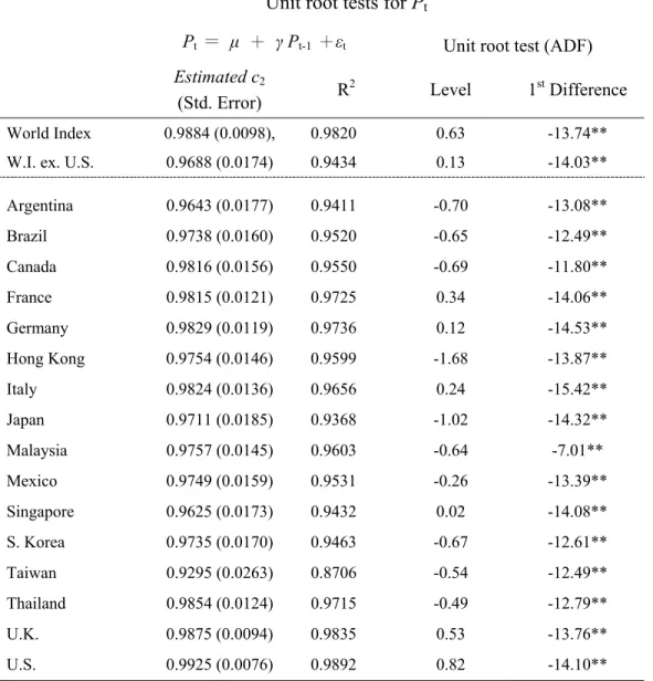
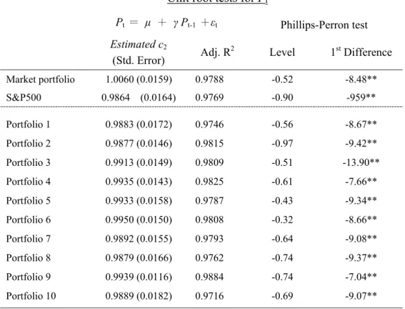
From equation (17), if price series follow a random walk process, then, the price series can be represented as Pt = Pt-1 + at, where at is a white noise. It follows
that Et-1Pt = Pt-1, EtPt+1=Pt and Et-1Pt+1=Pt-1. According the results in Appendix A1,
the assumption that price follows a random walk process seems to be reasonable for both data sets. As a result, equation (17) becomes
(18) - (r*cS-1 + A-1B) (Pt - Pt-1) + (cS-1 + A-1) (Et Dt+1 - Et-1 Dt+1) = Vt.
One can rewrite equation (18) as (19) G pt + H dt = Vt
where G = - (r*cS-1 + A-1B)
H = (cS-1+A-1)
dt = Et Dt+1 - Et-1 Dt+1
pt = Pt - Pt-1
If matrix G is assumed to be nonsingular, the reduced-form of the model may be written:
(20) pt = Π dt + Ut,
where Π is a n by n matrix of the reduced form coefficients and Ut is a column
vector of n reduced form disturbances. Or (21) Π= - G-1 H, and Ut = G-1 Vt.
Without a priori knowledge of the system, all equations of the model would look alike statistically in which each equation is a linear combination of all endogenous (pt) variables and all exogenous variables (dt). No equation contains
Thus, in estimating this model, it is necessary to assume that the expectation adjustments in dividends, dt, is exogenous in the model, i.e., dt is not
influenced by pt. However, before examining this assumption, it is also necessary
to model the dividend processes since the data used are in expectation terms and are not observable beforehand. Appendix A2 shows how to model the dividend processes for both data sets.
The results of this assumption are discussed in Appendix A3. From the Granger causality analysis, one can see that this assumption seems to be evidenced for most of the portfolios selected from S&P 500 or the country indices analyzed in this paper. Finally, the model can be estimated by the reduce form. The prices of value-weighted portfolio or the country indices series (pt) are
endogenous. In contrast, the series of expectation adjustments in dividend (dt)
will be treated as exogenous variable.
6. Test of Supply Effect
Since the simultaneous equation system as in equation (19) is exactly identified, it can be estimated by the reduced-form as equation (20). A proof of identification problem is shown in Appendix B. That is, equation (20), pt = Π dt +
Ut, can be used to test the supply effect. For example, in the case of two portfolios,
the coefficient matrix G and H in equation (19) can be written as3
(22) ⎥ ⎦ ⎤ ⎢ ⎣ ⎡ + − − − + − = ⎥ ⎦ ⎤ ⎢ ⎣ ⎡ = ) * ( * * ) * ( 2 2 22 21 12 1 1 11 22 21 12 11 b a cs r cs r cs r b a cs r g g g g G ⎥ ⎦ ⎤ ⎢ ⎣ ⎡ + + = ⎥ ⎦ ⎤ ⎢ ⎣ ⎡ = 2 22 21 12 1 11 22 21 12 11 a cs cs cs a cs h h h h H
Since Π= − G-1 H in equation (21), Πcan be calculated as
3s
ij is the ith row and jth column of the variance-covariance matrix of return. ai and bi are the supply
(23) ⎥ ⎦ ⎤ ⎢ ⎣ ⎡ + + ⎥ ⎦ ⎤ ⎢ ⎣ ⎡ + + = − − − 1 22 21 12 1 11 1 2 2 22 21 12 1 1 11 1 * * * * a cs cs cs a cs b a cs r cs r cs r b a cs r H G ⎥ ⎦ ⎤ ⎢ ⎣ ⎡ + + ⎥ ⎦ ⎤ ⎢ ⎣ ⎡ + − − + = 1 22 21 12 1 11 1 1 11 21 12 2 2 22 * * * * 1 a cs cs cs a cs b a cs r cs r cs r b a cs r G ⎢ ⎣ ⎡ + + + − − + + = 21 1 11 1 11 21 21 12 1 11 2 2 22 ) * ( ) ( * * ) )( * ( 1 cs b a cs r a cs cs r cs cs r a cs b a cs r G a ⎥ ⎦ ⎤ + + + − + − + ) )( * ( * ) ( * ) * ( 1 22 1 1 11 12 21 1 22 12 12 2 2 22 a cs b a cs r cs cs r a cs cs r cs b a cs r ⎥ ⎦ ⎤ ⎢ ⎣ ⎡ = 22 21 12 11 π π π π
From equation (23), if there is a high enough quadratic cost of adjustment, or if a1 = a2 = 0, then with s12 = s21, the matrix would become a scalar
matrix in which diagonal elements are equal to r*c2 (s11 s22 - s122), and the
off-diagonal elements are all zero. In other words, if there is high enough cost of adjustment, firm tends to stop seeking to raise new funds or to retire old securities. Mathematically, this will be represented in a way that all off-diagonal elements are all zero and all diagonal elements are equal to each other in matrix П. In general, this can be extended into the case of more portfolios. For example, in the case of N portfolios, equation (20) becomes
(24) . ⎥ ⎥ ⎥ ⎥ ⎦ ⎤ ⎢ ⎢ ⎢ ⎢ ⎣ ⎡ + ⎥ ⎥ ⎥ ⎥ ⎦ ⎤ ⎢ ⎢ ⎢ ⎢ ⎣ ⎡ ⎥ ⎥ ⎥ ⎥ ⎦ ⎤ ⎢ ⎢ ⎢ ⎢ ⎣ ⎡ = ⎥ ⎥ ⎥ ⎥ ⎦ ⎤ ⎢ ⎢ ⎢ ⎢ ⎣ ⎡ Nt t t Nt t t NN N N N N Nt t t u u u d d d p p p # # " # % # # " " # 2 1 2 1 2 1 2 22 21 1 12 11 2 1 π π π π π π π π π
Equation (24) shows that if an investor expects a change in the prediction of the next dividend due to the additional information, such as change in earnings, during the current period, then the price of the security changes. Regarding the international equity markets, if one believes that global financial market is perfectly integrated, that is, if one believes the way in which the expectation errors in dividends are built in the current price is the same for all
securities, then, the price changes would be influenced by only its own dividend expectation errors. Otherwise, say if the supply of securities is flexible, then the change in price would be influenced by the expectation adjustment in dividends of all other countries as well as that in its own dividend.
Therefore, two hypotheses related to supply effect are to be tested about the parameters in the reduced form system shown in equation (20).
Hypothesis 1: All the off-diagonal elements in the coefficient matrix Π are zero if the supply effect does not exist.
Hypothesis 2: All the diagonal elements in the coefficients matrix Π are equal in the magnitude if the supply effect does not exist.
These two hypotheses should be satisfied jointly. That is, if the supply effect does not exist, price changes of a security (index) should be a function of its own dividend expectation adjustments and the coefficients should be all equal across securities. In the model described in equation (18), if investor expects a change in the prediction of the next dividend due to the additional information during the current period, then the price of the security changes.
Under the assumption of the integration of the global financial market or the efficiency in the domestic stock market, the way in which the expectation errors in dividends are built in the current price is the same for all securities. This would happen if supply of securities is fixed and the price changes would be influenced by only its own dividend expectation errors. If the supply of securities is flexible, then the change in price would be influenced by the expectation adjustment in dividends of all other securities as well as that in its own dividend.
C Data and Empirical Results
In this Section, two different types of market are analyzed. First is the international equity market and the other is the U.S. domestic stock market. Most details of the model, the methodologies and the hypotheses for empirical tests have already discussed in Section B. However, before testing the hypotheses, some other details of the related tests that are needed to support the assumptions used in the model are also briefly discussed in this section. The first part of this section discusses the international asset pricing and second part, the domestic asset pricing in the U.S. stock market.
1 International Equity Markets – Country Indices
In this part, the existence of supply effect in the international equity markets will be tested. In other words, candidate explaining why the simple one-period static CAPM does not perform well is if supply effect exists in the global equity markets. The reason can also imply that a dynamic CAPM may be a better choice in international asset pricing model.
1.1 Data and Descriptive Statistics
The data used here comes from two different sources. One is the Global Financial Data in the Indexes and Databases of Rutgers Libraries and the second sets come from MSCI (Morgan Stanley Capital International, Inc.) equity indices. Most of the time the first data sets are used in all analyses, however, the second sets are sometimes used for comparison, for example, two sets are used in the Granger-causality test. The monthly data set consists of index, dividend yield, price earnings ratio and capitalization for each equity market. There are eighteen indices used, including G7, nine emerging markets, one world index and one other world index excluding the U. S. The list of all indices used is shown in Appendix C. For all countries, indices, dividends and earnings are all converted into U.S. dollar denominations. The exchange rate data also comes from Global Financial Data. These monthly series start from February 1988 to March 2004.
In Table 1.1, the first four moments of monthly returns of national indexes is reported. The emerging markets tend to be more volatile than developed markets though they may yield opportunity of higher return. The average of monthly variance of return in emerging markets is 0.166 while the average of monthly variance of return in developed countries is 0.042. Consider the coexistence of the low global correlation and high volatility in developing countries, the information from global markets are less sensitive to the investors in the domestic market but local news causes larger impact on equity prices.
1.2 Dynamic CAPM with Supply Side Effect
Recall the previous analysis, the structure form equations are exactly identified and the series of expectation adjustments in dividend, dt, are
exogenous variables. Now, the reduce form equations can be used to test the supply effect. That is, equation (24) needs to be examined by the following hypotheses:
Hypothesis 1: All the off-diagonal elements in the coefficient matrix Π are zero if the supply effect does not exist.
Hypothesis 2: All the diagonal elements in the coefficients matrix Π are equal in the magnitude if the supply effect does not exist.
These two hypotheses should be satisfied jointly. That is, if the supply effect does not exist, price changes of each country’s index would be a function of its own dividend expectation adjustments and the coefficients should be equal across all countries.
The estimated results of the simultaneous equations system are summarized in Table 1.2. The report here is from the estimates of seemingly unrelated regression (SUR) method.4 Under the assumption that the global
equity market consists of these sixteen counties, the estimations of diagonal elements vary across countries and some of the off-diagonal elements are
significant from zero. The results from G7 and the rest of the countries are also reported in Table 1.2-1 and Table 1.2-2. The elements in these two matrices are similar to the elements in matrix П. However, simply observing the elements in matrix П directly can not justify or reject the null hypotheses derived for testing the supply effect. Two tests should be done separately to check whether these two hypotheses can be both satisfied. For the first hypothesis, the test of supply effect on off-diagonal elements, the following regression is run for each country:
pi, t = βi di, t + Σj≠i βj dj, t + εi, t, i, j = 1, …,16. The null hypothesis then can be
written as: H0: βj = 0, j=1, …, 16, j ≠i. The results are reported in Table 1.3. Two
test statistics are reported. The first one is an F distribution with 15 and 172 degrees of freedom, and the second one is a chi-squared distribution with 15 degrees of freedom. Most countries have larger values of F-statistic and chi-squared statistic than the critic values. Thus, the null hypothesis is rejected at different levels of significance in most countries.
For the second test, the following null hypothesis needs to be tested: H0: πi,i = πj,j for all i, j=1, …, 16
Under the above fifteen restrictions, the Wald test statistic has a chi-square distribution with 15 degrees of freedom. The statistic is 165.03, which corresponds to a p-value of 0.000. One can reject the null hypothesis at any conventional levels of significance. In other words, the diagonal elements are obviously not similar to each other in magnitude. From these two tests, the two concerned hypotheses cannot be satisfied jointly, or, the non-existence of supply will be rejected. Thus, the empirical results suggest the existence of supply effect in international equity markets.
2 United States Equity Markets – S&P500
This part examines the hypotheses derived from Section B for the U.S. domestic stock market. Similar to the first part of this section, the focus is discussion of the existence of supply effect when market is assumed in
equilibrium. If the supply effect exists, this may imply that the U.S. stock market is not efficient. In other words, if the supply of risky assets is responsive to its price, large price changes, due to the change in expectation of future dividend, will be spread over time.
2.1 Data and Descriptive Statistics
Three hundred companies were selected from the S&P500 list and grouped into ten portfolios with equal numbers of thirty companies by their payout ratios. The data are obtained from the COMTUSTAT North America industrial quarterly data. The data starts from the first quarter of 1981 to the last quarter of 2002. The companies selected here should satisfy the following criteria. First, the company should appear or has appeared in S&P500 list during the period. Second, there are a complete data available, including price, dividend, earnings per share and shares outstanding, during the 88 quarters (22 years). The number of the company increases, though not much, if one allows those companies once listed in S&P500 but not in the current list. Some companies no longer exist, for example, are merged by others, or are excluded. The second criterion eliminates some of the current companies since they are new established. Some other firms are eliminated from the list because their report earnings or were trivial or even negative and dividend were trivial.5 314 firms
left after these adjustments. Finally, excluding those seven companies with highest and lowest average payout ratio, the rest are grouped into ten portfolios by the payout ratio. Each portfolio contains 30 companies. Figure 1 shows the comparison of S&P500 index and the value-weighted price of the market portfolio composed by the 300 firms selected. The path pattern is similar to each other before the 3rd quarter of 1999. That is, some volatile stocks are not included in the market portfolio with 300 firms.
In order to group these 300 firms, the payout ratio for each firm in each
5 The payout ratios here are computed each year and then average out over the entire 22 years. Thus,
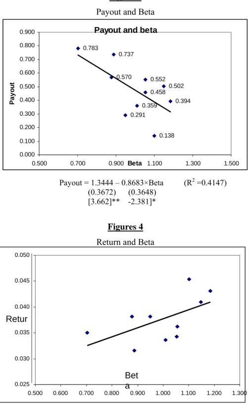
year is determined by dividing the sum of four quarters’ dividends by the sum of four quarters’ earnings, then, the yearly ratios are further averaged over the 22-year period. The first 30 firms with highest payout ratio comprises portfolio one, and so on, then, the price, dividend and earnings of each portfolio are computed by value-weighted of the 30 firms that are belonged to the same category. All the data of the market portfolio are derived from the value-weighted data of 10 portfolios. Some summary statistics of these 10 portfolios are described in Table 2.1 From Table 2.1 and Figure 2 to Figure 4, it appears to exist an inverse relationship between return and payout ratio, payout ratio and beta. However, the positive relationship between return and beta is not so clear.6 The average size of each portfolio does not seem to relate to the other
three factors. There are a lot of literatures regarding the relationships among the values of these factors; however, it is not a topic in this dissertation, though these figures show evidences consistent with some of the findings. The emphasis here is that each portfolio seems to be well characterized by their dividend payout ratio.
Table 2.2 shows the first four moments of quarterly returns of the market portfolio and ten portfolios. The coefficients of skewness, kurtosis, and Jarque-Bera statistics show that one can not reject the hypothesis that log return in most portfolios is normal.7 The fact shows that the kurtosis statistics for most
sample portfolios are close to three, which seems to imply no serious problem of heavier tails. Additionally, Jarque-Bera coefficients illustrate that the hypotheses of Gaussian distribution for most portfolios are not rejected. It seems to be unnecessary to consider the problem of heteroskedasticity in estimating domestic stock market if the quarterly data are used.
6 For example, Fama and French (1992) say their results seem to contradict the evidence that the slope of
the line relating expected return and beta is positive. Black (1993) argues the low-beta may continue to do better than CAPM says they should.
7 It should be noted that failing to reject normality does not confirm it. This test is only a test of symmetry
2.2 Dynamic CAPM with Supply Side Effect
If one believes that the stock market is efficient, that is, if one believes the way in which the expectation errors in dividends are built in the current price is the same for all securities, then, the price changes would be influenced by only its own dividend expectation errors. Otherwise, say, if the supply of securities is flexible, then the change in price would be influenced by the expectation adjustment in dividends of other portfolios as well as that in its own dividend. Thus, two hypotheses related to supply effect are to be tested and should be satisfied jointly in order to examine whether there exists a supply effect.
The estimated results of the simultaneous equations system are summarized in Table 2.3. The results are similar to each other by either using FIML or SUR approach. The report here is from the estimates of SUR method. If one assumes that stock market consists of ten portfolios used in this study, the supply effect seems to exist, but not significantly. The estimations of diagonal elements seem to vary across portfolios and most of the off-diagonal elements are significant from zero. Again, the null hypotheses can be tested by the tests mentioned in the previous section. The results of the test on off-diagonal elements are reported in Table 2.4. The null hypothesis is rejected at 5% level in six out of ten portfolios, but only two are rejected at 1% level. This evidence seems to be insufficient to reject the null hypothesis.
For the second one, the following null hypothesis needs to be tested. H0:
πi,i = πj,j for all i, j=1, …, 10. Under the above nine restriction, the Wald test
statistic has a chi-square distribution with nine degrees of freedom. The statistic is 18.858, which is greater than 16.92 at a significant level of 5%. Since the statistic corresponds to a p-value of 0.0265, one can reject the null hypothesis at 5% though it cannot reject H0 at a significant level of 1%. In other words, the
diagonal elements are not similar to each other in magnitude. In conclusion, the empirical results are sufficient to reject two null hypotheses of non-existence of supply effect in the U.S. stock market.
D. Summary and Concluding Remarks
In summary, the paper attempts to examine the asset pricing model which incorporates firm’s decision concerning the supply of risky securities into the CAPM. This model focuses on a firm’s capital decision by explicitly introducing the firm’s supply of risky securities into the static CAPM and allows supply of risky securities to be a function of security price. And thus, the expected returns are endogenously determined by both demand and supply decisions within the model. In other words, the supply effect may be one possible factor that can invalidate the implication of the traditional CAPM.
The objectives are to investigate the existence of supply effect in both international equity markets and U.S. stock markets. The test results show that two null hypotheses of non-existence of supply effect do not seem to be satisfied jointly in both data sets. In other words, this evidence seems to be sufficient to support the existence of supply effect, and thus, imply a violation of the assumption in the one period static CAPM, or imply a dynamic asset pricing model may be a better choice in both international equity markets and U.S. domestic stock markets.
However, some limitations should be mentioned. First, there is no discussion for the role of the exchange rate in the international pricing setting. In the analysis of international equity market, all the variables, such as index, dividends and earnings, are directly converted from local currency into U.S. dollars denominations. This is true only when the investors and firms are aware of the exact concurrent value of the local currency and able to buy or sell at this value as they are making decisions. In other words, it is true only when the foreign exchange markets in all countries are efficient. However, the structure of foreign exchange markets varies across the countries. Even in the same country, the structure changes over time. There exist huge differences in foreign exchange market before and after the deregulation of capital flow. To modify this, one needs to be very cautious on the changes of market structure in those emerging
markets since the data period analyzed covers the time when the foreign exchange markets change dramatically there.
The other problem is that the second alternative uses dollar returns instead of rate of return. This differs from the first alternative model or the traditional static CAPM. This limitation makes it difficult to compare the second alternative with the first model or with the static one. One way to modify this drawback is to normalize the dollar return to the conventional return measure by dividing it by the share price or index. However, this may lead to a nonlinearity problem among the variables in the derived demand and supply functions and complicates the relationship between price and quantity information. Some may question the second alternative for the assumption of an exogenous interest rate. A constant riskfree rate is indeed unrealistic, but this simplifies the analysis. The main reason why the interest rate is treated as constant is that changes in the interest rate are not important for the issue of supply effect.
Another problem could arise as one tries to apply this model into an international pricing model. The developed model is based on the decision of an individual firm and on the prices and dividends of individual security; however, there are structure differences among countries’ equity markets. Whether this theoretical model can extend to country indices needs some deeper investigations. For examples, firms were strictly restricted to buy back securities issued by themselves in some countries not long ago. The difficulty in issuing new funds or retiring old securities varies across countries, thus the costs of adjustment are in different scale for the firms located in the different countries. Nonetheless, the lift of restriction on fixed supply of risky security in the second alternative is an interesting and encouraging modification of the static CAPM. Fixed supply is one of the most restrictive assumptions underlying the CAPM. Change in supply of securities is related to investment decisions, capital structure, and dividend policy. Once the restriction disappears, the quantity supplied of risky securities starts to play a role in asset pricing.
Reference
Adler, M., and B. Dumas (1983), “International Portfolio Selection and Corporation Finance: A Synthesis,” Journal of Finance 38, 925-984.
Bekaert, G., C. R. Harvey, and Ng, A. (2003), “Market Integration and Contagion,”
NBER Working paper 9510 (EFA 2002 Berlin Meetings Presented Paper)
Black, Stanley W. (1976), “Rational Response to Shocks in a Dynamic model of Capital Asset Pricing,” American Economic Review 66, 767-779.
Black, F., M. Jensen, and M. Scholes (1972), “The Capital Asset Pricing Model: Some Empirical Tests,” in Jensen, M. (ed.), Studies in the Theory of Capital Markets, Praeger, New York, 79-121.
Breeden, D.T. (1979), “An Intertemporal Asset Pricing Model with Stochastic Consumption and Investment Opportunities,” Journal of Financial Economics 7, 265-196.
Brennan, M. J., A. W. Wang, and Xia, Y. (2004), “Estimation and Test of a Simple Model of Intertemporal Capital Asset Pricing,” Journal of Finance 59, 1743-1775. Campbell, John Y. (2000), “Assets Pricing at the Millennium,” Journal of Finance 55, 1515-1567.
Campbell, Lo, and MacKinlay (1997), The Econometrics of Financial Markets, Princeton University Press.
Campbell, John Y., Sanford J. Grossman and Jiang Wang (1993), “Trading Volume and Serial Correlation in Stock Returns,” Quarterly Journal of Economics 108, 905-939. Campbell, Harvey R., “Predictable Risk and Returns in Emerging Markets (1995),” Review of Financial Study, and NBER 4621.
Cochrane, John H. (2001), Asset Pricing, Princeton University Press.
Cox, John C., Jonathan E. Ingersoll, Jr., and Stephen A. Ross (1985), “An Intertemporal General Equilibrium Model of Asset Prices,” Econometrica 53, 363-384.
De Santis G., and B. Gerard (1997), “International Asset Pricing and Portfolio Diversification with Time-Varying Risk,” Journal of Finance 52, 1881-1912.
De Santis G., and B. Gerard (1998), “How Big is the Premium for Currency Risk”
Journal of Financial Economics 49, 375-412.
Dumas, B., and B. Solnik (1995), “The World Price of Foreign Exchange Risk,” Journal
of Financial Economics 50, 445-479.
Fama, E., and K. R. French (1992), “The Cross-section of Expected Stock Return,”
Fama, E., and K. R. French (1993), “Common Risk Factors in the Return on Bonds and Stocks,” Journal of Financial Economics 33, 3-56.
Fama, E., and K. R. French (1996), “Multifactor Explanations of Asset Pricing Anomalies,” Journal of Finance 51, 55-84.
Fama, E., and K. R. French (1998), “Value versus Growth: The International Evidence,”
Journal of Finance 53, 1975-1999.
Fama, E., and K. R. French (2000), “Disappearing Dividends: Changing Firm Characteristics or Lower Propensity to Pay?” Journal of Financial Economics 60, 3-43. Ferson, W. E., and C. R. Harvey (1991), “The Variation of Economic Risk Premiums,”
The Journal of Political Economy 99, 385-415.
Ferson, W. E., and C. R. Harvey (1999), “Conditioning Variables and the Cross Section of Stock Returns,” The Journal of Finance 54, 1325 – 1360.
Granger, C. W. J (1969), “Investigating Causal Relations by Econometric Models and Cross-spectral Methods,” Econometrica, vol. 37
Grinols, Earl L. (1984), “Production and Risk Leveling in the Intertemporal Capital Asset Pricing Model.” The Journal of Finance, Vol. 39, Issue 5, 1571-1595.
Grossman, Sanford J., and Zhongquan Zhou (1996), “Equilibrium Analysis of Portfolio Insurance,” Journal of Finance 51, 1379-1403.
Gweon, Seong Cheol (1985), “Rational Expectation, Supple Effect, and Stock Price Adjustment Process: A Simultaneous Equations System Approach,” Ph.D Dissertation, Univ. of Illinois.
Hansen, Lar Peter (1982), “Large Sample Properties of Generalized Method of Moments Estimators,” Econometrica 50, 1029-1054.
Harvey, C.R. (1991), “The World Price of Covariance Risk,” Journal of Finance 46, 111-158.
Hamilton, James D. (1994), “Time Series Analysis,” Princeton University Press.
Lee, Cheng-few, and Seong Cheol Gweon (1986), “Rational Expectation, Supply Effect and Stock Price Adjustment,” paper presented at Econometrica Society annual meeting 1986.
Lee, Cheng-few, and Chunchi Wu, and Mohamed Djarraya (1987), “A Further Empirical Investigation of the Dividend Adjustment Process,” Journal of Econometrics 35, 267-285.
Lintner, J. (1965), “The Valuation of Risky Assets and the Selection of Risky Investments in Stock Portfolios and Capital Budgets,” Review of Economics and
Lo, Andrew W., and Jiang Wang (2000), “Trading Volume: Definition, Data Analysis, and Implications of Portfolio Theory,” Review of Financial Studies 13, 257-300.
Markowitz, H. (1959), Portfolio Selection: Efficient Diversification of Investments, John Wiley, New York.
Mehra, Rajnish, and Prescott Edward (1985), “The Equity Premium: A Puzzle,” Journal
of Monetary Economics 15, 145-161.
Merton, Robert C. (1973), “An Intertemporal Capital Assets Pricing Model,”
Econometrica, 41, 867-887.
Mossin, J. (1966), “Equilibrium in a Capital Asset Market,” Econometrica 35, 768-783. Ross, Stephen A. (1976), “The Arbitrage Theory of Capital Asset Pricing,” Journal of
Economic Theory 13, 341-360.
Sharpe, W. (1964), “Capital Asset Prices: A Theory of Market Equilibrium under Conditions of Risk,” Journal of Finance 19, 425-442.
Solnik, Richard E. (1974), “An Equilibrium Model of the International Capital Market,”
Journal of Economic Theory 8, 500-524.
Stulz, R. (1981), “A Model of International Asset Pricing,” Journal of Financial
Economics 9, 383-406.
Wang, Q. K. (2003), “Asset Pricing with conditional Information: A New Test,” The Journal of Finance 58, 161 – 196.
Table 1.1
Summary Statistics of Monthly Return
Country (Monthly) Mean (Monthly)Std. Dev. Skewness Kurtosis Jarque-Bera
WI 0.0051 0.0425 -0.3499 3.3425 4.7547 WI excl.US 0.0032 0.0484 -0.1327 3.2027 0.8738 CD 0.0064 0.0510 -0.6210 4.7660 36.515** FR 0.0083 0.0556 -0.1130 3.1032 0.4831 GM 0.0074 0.0645 -0.3523 4.9452 33.528** IT 0.0054 0.0700 0.2333 3.1085 1.7985 JP -0.00036 0.0690 0.3745 3.5108 6.4386* UK 0.0056 0.0474 0.2142 3.0592 1.4647 US 0.0083 0.0426 -0.3903 3.3795 5.9019
Country (Monthly) Mean (Monthly)Std. Dev. Skewness Kurtosis Jarque-Bera AG 0.0248 0.1762 1.9069 10.984 613.29** BZ 0.0243 0.1716 0.4387 6.6138 108.33** HK 0.0102 0.0819 0.0819 4.7521 26.490** KO 0.0084 0.1210 1.2450 8.6968 302.79** MA 0.0084 0.0969 0.5779 7.4591 166.22** MX 0.0179 0.0979 -0.4652 4.0340 15.155** SG 0.0072 0.0746 -0.0235 4.8485 26.784** TW 0.0092 0.1192 0.4763 4.0947 16.495** TL 0.0074 0.1223 0.2184 4.5271 19.763**
1. The monthly returns from Feb. 1988 to March 2004 for international markets. 2. * and ** denote statistical significance at the 5% and 1%, respectively.
Table 1.2
Coefficients for matrix П (all sixteen markets)
P_CD P_FR P_GM P_IT P_JP P_UK P_US P_TW P_TH P_SG P_MX P_MA P_KO P_HK P_BZ P_AG 0.416 0.626 0.750 0.232 0.608 0.233 0.282 0.130 0.066 1.003 1.130 0.126 0.035 3.080 0.564 1.221 (0.087) (0.137) (0.183) (0.055) (0.481) (0.095) (0.108) (0.095) (0.089) (0.388) (0.317) (0.061) (0.035) (1.049) (0.209) (0.392) [ 4.786] [ 4.570] [ 4.106] [ 4.210] [ 1.264] [ 2.460] [ 2.623] [ 1.376] [ 0.743] [ 2.583] [ 3.560] [ 2.056] [ 1.010] [ 2.935] [ 2.698] [ 3.114] 0.003 0.038 0.015 -0.008 0.067 -0.015 0.001 -0.036 -0.027 -0.170 -0.144 -0.030 0.012 -0.067 -0.020 -0.110 (0.021) (0.034) (0.045) (0.014) (0.119) (0.023) (0.027) (0.023) (0.022) (0.096) (0.078) (0.015) (0.009) (0.259) (0.052) (0.097) [ 0.145] [ 1.121] [ 0.342] [-0.585] [ 0.567] [-0.650] [ 0.024] [-1.522] [-1.247] [-1.771] [-1.845] [-1.968] [ 1.347] [-0.260] [-0.390] [-1.137] -15.03 40.376 43.677 8.090 -6.208 9.340 -28.52 -8.987 2.107 -79.09 -78.51 2.538 -4.437 -75.61 13.109 -54.23 (19.51) (30.78) (41.05) (12.39) (108.1) (21.27) (24.16) (21.23) (20.04) (87.20) (71.29) (13.76) (7.84) (235.7) (46.91) (88.09) [-0.771] [ 1.312] [ 1.064] [ 0.653] [-0.057] [ 0.439] [-1.181] [-0.423] [ 0.105] [-0.907] [-1.101] [ 0.184] [-0.566] [-0.321] [ 0.279] [-0.616] 0.043 0.029 0.062 0.099 -0.030 0.022 0.014 0.000 0.014 0.155 0.275 -0.024 0.002 0.455 0.043 0.272 (0.043) (0.069) (0.091) (0.028) (0.241) (0.047) (0.054) (0.047) (0.045) (0.194) (0.159) (0.031) (0.017) (0.525) (0.104) (0.196) [ 0.980] [ 0.427] [ 0.683] [ 3.585] [-0.124] [ 0.473] [ 0.265] [-0.002] [ 0.321] [ 0.799] [ 1.730] [-0.789] [ 0.115] [ 0.867] [ 0.413] [ 1.390] 0.058 0.087 0.073 0.020 0.801 0.069 0.083 0.035 0.012 0.173 0.203 -0.003 0.023 0.466 0.086 0.080 (0.015) (0.024) (0.032) (0.010) (0.084) (0.017) (0.019) (0.016) (0.016) (0.068) (0.055) (0.011) (0.006) (0.183) (0.036) (0.068) [ 3.842] [ 3.641] [ 2.300] [ 2.101] [ 9.537] [ 4.205] [ 4.396] [ 2.132] [ 0.746] [ 2.558] [ 3.668] [-0.242] [ 3.777] [ 2.546] [ 2.366] [ 1.173] -22.313 29.783 13.186 -7.778 99.863 127.70 -23.812 -43.206 -14.772 28.205 -23.034 20.639 -15.315 -23.313 -58.263 -72.967 (24.88) (39.25) (52.36) (15.80) (137.9) (27.13) (30.82) (27.08) (25.56) (111.2) (9.09) (17.55) (10.00) (30.06) (59.83) (112.4) [-0.897] [ 0.759] [ 0.252] [-0.492] [ 0.724] [ 4.707] [-0.773] [-1.595] [-0.578] [ 0.254] [-2.533] [ 1.176] [-1.532] [-0.776] [-0.974] [-0.649] -29.480 -54.442 -56.122 -17.049 -61.119 -29.977 -23.036 -22.029 35.898 -80.345 -74.468 -25.152 -0.222 -18.695 -22.574 -82.626 (12.70) (20.04) (26.73) (8.07) (70.42) (13.85) (15.73) (13.82) (13.05) (56.77) (46.42) (89.61) (51.02) (15.35) (30.54) (57.35) [-2.287] [-2.717] [-2.100] [-2.114] [-0.868] [-2.165] [-1.464] [-0.159] [ 0.275] [-1.415] [-1.604] [-0.281] [-0.004] [-1.218] [-0.739] [-1.441] -0.041 0.000 0.026 0.028 -0.070 -0.008 -0.038 0.030 -0.068 -0.280 -0.080 0.017 -0.030 -0.957 0.105 -0.407 (0.065) (0.102) (0.136) (0.041) (0.359) (0.071) (0.080) (0.071) (0.067) (0.290) (0.237) (0.046) (0.026) (0.783) (0.156) (0.293) [-0.634] [-0.004] [ 0.188] [ 0.684] [-0.194] [-0.120] [-0.479] [ 0.426] [-1.025] [-0.965] [-0.338] [ 0.361] [-1.138] [-1.222] [ 0.677] [-1.390] -0.026 -0.050 -0.020 -0.035 0.021 -0.056 -0.068 0.017 0.031 0.099 -0.176 0.074 -0.001 -0.011 -0.022 -0.190 (0.032) (0.050) (0.067) (0.020) (0.177) (0.035) (0.040) (0.035) (0.033) (0.143) (0.117) (0.023) (0.013) (0.386) (0.077) (0.144) [-0.820] [-0.987] [-0.295] [-1.722] [ 0.117] [-1.608] [-1.727] [ 0.494] [ 0.943] [ 0.692] [-1.508] [ 3.280] [-0.059] [-0.028] [-0.284] [-1.315] 0.025 0.039 0.017 0.008 0.028 0.031 0.039 0.029 0.023 0.222 0.050 0.018 0.008 0.479 0.048 0.078 (0.015) (0.024) (0.032) (0.010) (0.084) (0.017) (0.019) (0.017) (0.016) (0.068) (0.056) (0.011) (0.006) (0.184) (0.037) (0.069) [ 1.613] [ 1.623] [ 0.516] [ 0.854] [ 0.334] [ 1.867] [ 2.082] [ 1.737] [ 1.465] [ 3.264] [ 0.906] [ 1.666] [ 1.257] [ 2.606] [ 1.325] [ 1.134] 0.011 0.024 0.034 0.003 -0.037 0.017 0.022 0.011 0.012 0.085 0.184 0.002 0.006 0.286 0.053 0.080 (0.009) (0.015) (0.020) (0.006) (0.052) (0.010) (0.012) (0.010) (0.010) (0.042) (0.034) (0.007) (0.004) (0.114) (0.023) (0.043) [ 1.189] [ 1.644] [ 1.736] [ 0.423] [-0.705] [ 1.672] [ 1.887] [ 1.033] [ 1.212] [ 2.018] [ 5.341] [ 0.248] [ 1.492] [ 2.518] [ 2.323] [ 1.886] 0.019 -0.110 -0.064 -0.026 0.304 0.048 -0.019 -0.073 0.011 0.018 -0.060 0.057 0.009 -0.160 -0.160 -0.344 (0.070) (0.111) (0.148) (0.045) (0.389) (0.077) (0.087) (0.076) (0.072) (0.314) (0.257) (0.050) (0.028) (0.848) (0.169) (0.317) [ 0.276] [-0.992] [-0.431] [-0.590] [ 0.780] [ 0.628] [-0.224] [-0.958] [ 0.150] [ 0.059] [-0.234] [ 1.160] [ 0.333] [-0.189] [-0.947] [-1.085] 0.103 0.071 -0.077 0.037 1.007 0.070 0.176 -0.005 0.029 0.449 0.077 -0.045 0.158 -0.726 -0.071 0.102 (0.082) (0.129) (0.172) (0.052) (0.453) (0.089) (0.101) (0.089) (0.084) (0.365) (0.299) (0.058) (0.033) (0.987) (0.196) (0.369) [ 1.262] [ 0.548] [-0.446] [ 0.706] [ 2.225] [ 0.782] [ 1.740] [-0.060] [ 0.345] [ 1.230] [ 0.257] [-0.789] [ 4.818] [-0.736] [-0.362] [ 0.278] -0.012 -0.013 -0.008 -0.006 -0.013 -0.007 -0.009 0.003 -0.001 -0.021 -0.006 -0.001 -0.002 -0.006 -0.012 -0.008 (0.004) (0.007) (0.009) (0.003) (0.024) (0.005) (0.005) (0.005) (0.004) (0.019) (0.016) (0.003) (0.002) (0.053) (0.010) (0.020) [-2.844] [-1.921] [-0.891] [-2.158] [-0.540] [-1.549] [-1.736] [ 0.568] [-0.113] [-1.083] [-0.359] [-0.331] [-1.209] [-0.112] [-1.123] [-0.386] 0.009 0.017 0.023 0.005 -0.012 0.012 0.016 0.008 -0.003 0.012 0.050 0.004 0.000 0.017 0.053 0.060 (0.005) (0.007) (0.010) (0.003) (0.025) (0.005) (0.006) (0.005) (0.005) (0.020) (0.017) (0.003) (0.002) (0.055) (0.011) (0.021) [ 1.878] [ 2.337] [ 2.424] [ 1.855] [-0.490] [ 2.328] [ 2.907] [ 1.568] [-0.557] [ 0.605] [ 2.989] [ 1.226] [-0.068] [ 0.306] [ 4.801] [ 2.902] 0.007 0.008 0.008 0.001 -0.001 0.008 0.008 0.001 0.005 0.000 0.049 0.002 0.000 0.061 0.009 0.094 (0.005) (0.007) (0.010) (0.003) (0.026) (0.005) (0.006) (0.005) (0.005) (0.021) (0.017) (0.003) (0.002) (0.056) (0.011) (0.021) [ 1.466] [ 1.056] [ 0.857] [ 0.356] [-0.025] [ 1.614] [ 1.326] [ 0.255] [ 1.012] [-0.004] [ 2.879] [ 0.604] [-0.017] [ 1.081] [ 0.776] [ 4.464] 0.3148 0.31 0.2111 0.2741 0.4313 0.3406 0.2775 0.1241 0.0701 0.2148 0.3767 0.1479 0.2679 0.1888 0.2435 0.2639 5.2676 5.151 3.0692 4.3299 8.6948 5.9235 4.4049 1.6245 0.8642 3.1376 6.9313 1.9898 4.196 2.6688 3.69 4.1112
Table 1.2-1
Coefficients for matrix П (G7 countries)
CD FR GM IT JP UK US Canada (CD) 0.4285 0.6293 0.7653 0.2302 0.5960 0.2415 0.2877 (0.0887) (0.1387) (0.1815) (0.0553) (0.4722) (0.0964) (0.1114) [ 4.83222] [ 4.53805] [ 4.21660] [ 4.16284] [ 1.26211] [ 2.50434] [ 2.58267] France (FR) 0.0092 0.0479 0.0224 -0.0069 0.0659 -0.0132 0.0037 (0.0211) (0.0331) (0.0433) (0.0132) (0.1126) (0.0230) (0.0265) [ 0.43450] [ 1.45043] [ 0.51768] [-0.52404] [ 0.58564] [-0.57310] [ 0.14092] German (GM) -22.2372 27.6389 29.0424 5.7762 -17.3229 1.3207 -42.1272 (19.7482) (30.8842) (40.4215) (12.3171) (105.1662) (21.4773) (24.8064) [-1.12604] [ 0.89492] [ 0.71849] [ 0.46895] [-0.16472] [ 0.06149] [-1.69824] Italy (IT) 0.0522 0.0371 0.0799 0.1043 0.0342 0.0318 0.0330 (0.0432) (0.0676) (0.0884) (0.0269) (0.2300) (0.0470) (0.0543) [ 1.20922] [ 0.54894] [ 0.90383] [ 3.87215] [ 0.14853] [ 0.67670] [ 0.60883] Japan (JP) 0.0738 0.1040 0.0864 0.0245 0.8312 0.0836 0.0996 (0.0149) (0.0234) (0.0306) (0.0093) (0.0796) (0.0163) (0.0188) [ 4.93698] [ 4.45014] [ 2.82459] [ 2.63259] [ 10.4454] [ 5.14208] [ 5.30466] U. K. (UK) -40.7615 -0.8139 -16.2433 -16.6896 112.3044 112.3671 -44.9229 (24.8303) (38.8320) (50.8237) (15.4869) (132.2300) (27.0043) (31.1901) [-1.64160] [-0.02096] [-0.31960] [-1.07766] [ 0.84931] [ 4.16109] [-1.44029] U. S. (US) -31.2190 -56.8336 -57.4718 -15.7037 -71.5680 -30.7517 -26.3700 (12.8501) (20.0963) (26.3022) (8.0147) (68.4315) (13.9752) (16.1415) [-2.42947] [-2.82807] [-2.18506] [-1.95935] [-1.04583] [-2.20045] [-1.63368] R-squared 0.2294 0.2373 0.1605 0.2122 0.4095 0.2622 0.1641 F-statistic 8.9794 9.3872 5.7685 8.1274 20.9187 10.7183 5.9233
Table 1.2-2
Coefficients for matrix П (Nine emerging markets)
TW TH SG MX MA KO HK BZ AG Taiwan 0.0279 -0.0686 -0.3535 -0.1396 0.0040 -0.0258 -1.1395 0.0761 -0.5048 (TW) (0.0709) (0.0652) (0.2943) (0.2548) (0.0454) (0.0265) (0.7956) (0.1573) (0.2966) [ 0.39388] [-1.05234] [-1.20100] [-0.54785] [ 0.08857] [-0.97462] [-1.43238] [ 0.48390] [-1.70195] Thailand 0.0167 0.0263 0.1122 -0.1344 0.0660 0.0068 0.1445 0.0008 -0.1593 (TH) (0.0344) (0.0316) (0.1428) (0.1236) (0.0220) (0.0129) (0.3859) (0.0763) (0.1439) [ 0.48456] [ 0.83246] [ 0.78605] [-1.08725] [ 2.99283] [ 0.53054] [ 0.37457] [ 0.01022] [-1.10720] Singapore 0.0315 0.0215 0.2163 0.0524 0.0142 0.0120 0.4915 0.0519 0.0574 (SG) (0.0162) (0.0149) (0.0674) (0.0584) (0.0104) (0.0061) (0.1822) (0.0360) (0.0679) [ 1.93909] [ 1.44098] [ 3.20829] [ 0.89816] [ 1.36499] [ 1.98318] [ 2.69713] [ 1.43966] [ 0.84543] Mexico 0.0133 0.0129 0.0923 0.1955 0.0025 0.0049 0.2794 0.0503 0.0864 (MX) (0.0102) (0.0094) (0.0425) (0.0368) (0.0066) (0.0038) (0.1149) (0.0227) (0.0428) [ 1.30151] [ 1.37317] [ 2.17164] [ 5.31170] [ 0.37451] [ 1.26819] [ 2.43220] [ 2.21608] [ 2.01656] Malaysia -0.0668 0.0227 0.1107 -0.0168 0.0664 0.0106 -0.0391 -0.1358 -0.3029 (MA) (0.0760) (0.0699) (0.3154) (0.2731) (0.0487) (0.0284) (0.8526) (0.1686) (0.3179) [-0.87856] [ 0.32527] [ 0.35080] [-0.06150] [ 1.36417] [ 0.37456] [-0.04584] [-0.80543] [-0.95281] S. Korea 0.0040 0.0302 0.5954 0.2211 -0.0516 0.1724 -0.3149 -0.0105 0.2073 (KO) (0.0891) (0.0819) (0.3696) (0.3200) (0.0571) (0.0333) (0.9991) (0.1976) (0.3725) [ 0.04516] [ 0.36871] [ 1.61091] [ 0.69078] [-0.90507] [ 5.17701] [-0.31514] [-0.05290] [ 0.55646] HongKong 0.0008 -0.0011 -0.0262 -0.0176 -0.0003 -0.0033 -0.0287 -0.0161 -0.0124 (HK) (0.0047) (0.0043) (0.0196) (0.0170) (0.0030) (0.0018) (0.0530) (0.0105) (0.0198) [ 0.16463] [-0.25388] [-1.33665] [-1.03852] [-0.10295] [-1.88424] [-0.54139] [-1.53139] [-0.62961] Brazil 0.0091 -0.0020 0.0176 0.0621 0.0034 0.0005 0.0380 0.0558 0.0686 (BZ) (0.0049) (0.0045) (0.0205) (0.0177) (0.0032) (0.0018) (0.0554) (0.0110) (0.0206) [ 1.84521] [-0.43841] [ 0.85699] [ 3.50359] [ 1.08063] [ 0.28347] [ 0.68631] [ 5.09912] [ 3.32283] Argentina 0.0026 0.0050 0.0092 0.0585 0.0024 0.0012 0.0950 0.0154 0.1004 (AG) (0.0050) (0.0046) (0.0209) (0.0181) (0.0032) (0.0019) (0.0565) (0.0112) (0.0211) [ 0.51493] [ 1.08871] [ 0.44123] [ 3.23312] [ 0.74046] [ 0.65121] [ 1.68184] [ 1.37500] [ 4.76894] R-squared 0.057384 0.050263 0.137001 0.231799 0.104100 0.191448 0.108119 0.179049 0.194793 F-statistic 1.362139 1.184153 3.552016 6.751474 2.599893 5.297943 2.712414 4.879985 5.412899 Numbers in () are standard deviations, in [ ] are the t-value.
Table 1.3
Test of Supply Effect on off-Diagonal Elements of Matrix П
R 2 F- statistic p-value Chi-square p-value
Canada 0.3147 3.5055 0.0000 52.5819 0.0000 France 0.3099 4.6845 0.0000 70.2686 0.0000 German 0.2111 2.8549 0.0005 42.8236 0.0002 Italy 0.2741 2.9733 0.0003 44.6004 0.0001 Japan 0.4313 0.7193 0.7628 10.7894 0.7674 U.K. 0.3406 3.9361 0.0000 59.0413 0.0000 U.S. 0.2775 4.5400 0.0000 68.1001 0.0000 Taiwan 0.1241 1.6266 0.0711 24.3984 0.0586 Thailand 0.0701 0.7411 0.7401 11.1171 0.7442 Singapore 0.2148 2.1309 0.0106 31.9634 0.0065 Mexico 0.3767 4.7873 0.0000 71.8099 0.0000 Malaysia 0.1479 1.6984 0.0550 25.4755 0.0439 S. Korea 0.2679 2.1020 0.0118 31.5305 0.0075 Hongkong 0.1888 2.6836 0.0011 40.2540 0.0004 Brazil 0.2435 1.9174 0.0244 28.7613 0.0173 Argentina 0.2639 2.6210 0.0014 39.3155 0.0006 Note: 1. pi, t = βi’di, t + Σj≠i βj’dj, t + ε’i, t, i, j = 1, …,16.
Null Hypothesis: all βj = 0, j=1,…, 16, j ≠i
2. The first one is an F distribution with 15 and 172 degrees of freedom, and the second one is a chi-squared distribution with 15 degrees of freedom.
Table 2.1
Characteristics of Ten Portfolios
Portfolio Return Payout Size (000) Beta (M)
1 0.0351 0.7831 193,051 0.7028 2 0.0316 0.7372 358,168 0.8878 3 0.0381 0.5700 332,240 0.8776 4 0.0343 0.5522 141,496 1.0541 5 0.0410 0.5025 475,874 1.1481 6 0.0362 0.4578 267,429 1.0545 7 0.0431 0.3944 196,265 1.1850 8 0.0336 0.3593 243,459 1.0092 9 0.0382 0.2907 211,769 0.9487 10 0.0454 0.1381 284,600 1.1007
1. The first 30 firms with highest payout ratio comprises portfolio one, and so on.
2. The payout ratio for each firm in each year is found by dividing the sum of four quarters’ dividends by the sum of four quarters’ earnings, then, the yearly ratios are further averaged over the 22-year period.
3. The price, dividend and earnings of each portfolio are computed by value-weighted of the 30 firms included in the same category.
Table 2.2
Summary Statistics of Quarterly Return
Country (quarterly)Mean (quarterly)Std. Dev. Skewness Kurtosis Jarque-Bera Market portfolio 0.0364 0.0710 -0.4604 3.9742 6.5142* Portfolio 1 0.0351 0.0683 -0.5612 3.8010 6.8925* Portfolio 2 0.0316 0.0766 -1.1123 5.5480 41.470** Portfolio 3 0.0381 0.0768 -0.3302 2.8459 1.6672* Portfolio 4 0.0343 0.0853 -0.1320 3.3064 0.5928 Portfolio 5. 0.0410 0.0876 -0.4370 3.8062 5.1251 Portfolio 6. 0.0362 0.0837 -0.2638 3.6861 2.7153 Portfolio 7 0.0431 0.0919 -0.1902 3.3274 0.9132 Portfolio 8 0.0336 0.0906 0.2798 3.3290 1.5276 Portfolio 9 0.0382 0.0791 -0.2949 3.8571 3.9236 Portfolio 10 0.0454 0.0985 -0.0154 2.8371 0.0996
1. Quarterly returns from 1981:Q1to 2002:Q4 are calculated.