針對不受相位光罩長度限制的製作新方法分析密波長多工多通道光纖光柵濾波器頻譜干擾之最佳化修正

國立交通大學

光電工程研究所

碩士論文

針對不受相位光罩長度限制的

製作新方法分析密波長多工多通道光纖

光柵濾波器頻譜干擾之最佳化修正

Optimized spectral distortion correction of

DWDM multichannel FBG filters for

a new fabrication method not limited by the

phase mask length

研究生：辛宸瑋

指導教授：賴暎杰博士

中華民國九十七年七月

針對不受相位光罩長度限制的製作新方法分析密波長多工多通道光

纖光柵濾波器頻譜干擾之最佳化修正

Optimized spectral distortion correction of

DWDM multichannel FBG filters for a

new fabrication method not limited by the phase mask length

研 究 生：辛宸瑋 Student：Chen-Wei Hsin

指導教授：賴暎杰博士 Advisor：Dr. Yinchieh Lai

國 立 交 通 大 學

光 電 工 程 研 究 所

碩 士 論 文

A Thesis

Submitted to Institute of Electronics College of Engineering National Chiao Tung University

in partial Fulfillment of the Requirements for the Degree of

Master

In Electro-Optical Engineering July 2008

Hsinchu, Taiwan, Republic of China

摘 要

論文名稱：針對不受相位光罩長度限制的製作新方法分析密波長多工多通道光 纖光柵濾波器頻譜干擾之最佳化修正 校所別：國立交通大學光電工程研究所 頁數：61 頁 畢業時間：九十六學年度第二學期 學位：碩士 研究生：辛宸瑋 指導教授：賴暎杰 老師 關鍵詞：光纖光柵、側面繞射位置監控 本論文提出密波長多工多通道光纖光柵濾波器頻譜干擾之最佳化修正方法。 先利用其它可能引起頻譜干擾的多通道光纖光柵設計方法做初步設計，接著利用 Lagrange multiplier optimization(LMO)最佳化演算法來達到降低頻譜干擾的最 佳化設計。由於原先的設計已提供相當接近的折射率變化輪廓，使得利用 LMO 進 行最佳化運算時只需微小變化原先設計的輪廓便能快速收斂至目標反射頻譜，同 時此混合演算方法又能保留原先設計方法的優點，例如重疊寫入多通道光纖光柵 之易於製造的特色。本論文中我們也提出一種不受相位光罩長度限制的光纖光柵 製造平台構想並針對之來分析前面所設計出來的密波長多工多通道光纖光柵在實 際製造上之容忍誤差。此種藉由相位光罩一段一段接續的光纖光柵製造平台，應 能大大提升實際製造長度很長或是較複雜之光纖光柵的容忍誤差。

ABSTRACT

Title：Optimized spectral distortion correction of DWDM multichannel FBG filters for a new fabrication method not limited by the phase mask length

Pages：61 Page

School：National Chiao Tung University

Department：Institute of Electro-Optical Engineering

Time：July, 2008 Degree：Master

Researcher：Chen-Wei Hsin Advisor：Prof. Yin-Chieh Lai Keywords：Fiber Bragg Grating、Side-Diffraction Position Monitoring

This thesis presents work on optimized spectral distortion correction of DWDM multichannel fiber Bragg grating (FBG) filters. The developed hybrid algorithm starts from some other multichannel FBG design method which may suffer from the spectral distortion and use the Lagrange multiplier optimization (LMO) algorithm for final optimization. Due to the initially close-to-optimum index modulation profile, the calculation can be fast converged to the target reflection spectra by using the LMO algorithm and the final design still retains the merits of easy fabrication. We have also proposed a new fabrication method not limited by the phase mask length and have performed the tolerance analysis for the designed DWDM multichannel fiber Bragg grating (FBG) filters based on the proposed fabrication platform. By the section-by-section connection of the phase mask, this platform should effectively reduce the errors during the UV exposure and accurately fabricate FBG devices with long length and complicated profiles.

ACKNOWLEDGEMENT

這篇論文的完成最先感謝賴暎杰老師，在我研究過程中給予的指導，老師 猶如春風化雨澆灌我們，其敏銳的思考和廣博的學問令學生我興起敬仰之意， 在許多為人處世上的智慧也是我們的模範，在老師身上學到很多，總之很高興 能當老師的學生。 接著我感謝李澄鈴老師對於最佳化理論的指導，使我猶如在渾沌中找到一 盞明燈，在碩士短短的時間內明瞭其原理。另外也感謝許立根老師、莊凱評先 生在光纖光學實驗室所撰寫的程式，使我的程式能站在前人寫好的程式碼上作 修改，減少了一切重頭開始的苦功夫。 在口試期間, 承蒙口試委員祁甡教授、陳智弘教授以及彭朋群教授撥冗指 導並提供許多寶貴的意見,使此論文能更臻於完善,在此也誠摯地感謝您們的 辛勞。 同時，感謝陳南光老師和許宜蘘學姊對於我研究相關領域的教導，使我置 身在充滿學術氣氛與研究討論的環境中，並從中得到許多寶貴的建議。以及徐 桂珠學姐對於機台操作經驗之教導，和提供實驗室相關的資料，使我在研究相 關領域上亦受益良多。感謝項維巍老師、實驗室同學莊佩蓁、張宏傑，和學弟 妹池昱勳、鍾佩芳、顏子翔在課業和生活上的互相幫忙照顧，還有帶來的實驗 室樂趣。 感謝家人在我碩士這一路上的精神支持，尤其是在背後默默支持我的父母 親，對於你們全力的支持與關愛，僅致上無限的敬意與感激。最後感謝上天， 引領我完成碩士階段。

CONTENTS

Page

Abstract (in Chinese)

I

Abstract (in English)

II

Acknowledgement

III

Contents

IV

List of Figures

VI

Chapter 1 :

Introduction

1.1 Multichannel fiber Bragg grating 1

1.2 Motivation and purpose of the research 2

1.3 Structure of this thesis 4

1.4 References 5

Chapter 2 :

Background of the research 2.1 Theories 8

2.1-1 Coupled-mode theory 8

2.1-2 Transfer matrix method 12

2.1-3 Discrete layer-peeling method 14

2.1-4 Lagrange multiplier optimization method 17

2.2 Fabrication methods 21

2.2-1 Sequential UV writing techniques 21

2.2-2 Real-time interferometric side-diffraction position monitoring by probing the reference fiber grating 22 2.2-3 Real-time interferometric side-diffraction position monitoring by probing the reference phase mask 23 2.2-4 Least square error fitting method for determining the exposure parameters 31 2.3 References 32

Chapter 3 :

Principles of the research

3.1 LMO algorithm for optimization correction of superimposed FBG design

33 3.2 A new fabrication method not limited by the phase

mask length

Chapter 4 :

Results and discussion of the research

4.1 Discussion of optimization correction results 42 4.2 Tolerance analyses 44

Chapter 5 :

Conclusions and Future work

5.1 Conclusions 60

5.2 Future work

LIST OF FIGURES

Chapter 2

Fig. 1 The propagation modes in the general fiber. ...8

Fig. 2 The propagation modes in fiber grating. ...9

Fig. 3 The mode is exactly entering the perturbed index...9

Fig. 4 The forward and backward amplitude in FBG. ...12

Fig. 5 The discrete model of fiber Bragg grating ...14

Fig. 6 γ1(δ) can be thought as the sum of impulse responses from every reflector ...15

Fig. 7 The forward and backward amplitude in FBG. ...17

Fig. 8 A complex refractive index change fiber grating and the sequential writing techniques ...21

Fig. 9 The interference phase match for each step ...21

Fig. 10 The easy-looking figure of the real-time interferometric side-diffraction position monitoring by probing the reference fiber grating ...25

Fig. 11 The interference setup and pattern on CCD ...26

Fig. 12 The computer analyzes the real time interference pattern...26

Fig. 13 The computer feedback controls the PZT for achieving phase match ...27

Fig. 14 Illustration of fabrication procedures ...27

Fig. 15 Examples of FBG fabricated ...28

Fig. 16 Method to produce the reference FBG ...28

Fig. 17 Result of 0 percent period mismatch between the writing beam and the reference FBG ...29 Fig. 18 Results of 5 and 10 percent period mismatch between the writing

beam and the reference FBG ...29 Fig. 19 Real-time interferometric side-diffraction position monitoring by

probing the reference phase mask...30 Fig. 20 Example of FBG fabricated...30

Chapter 3、4

Fig. 1 Example of three channel superimposing...34 Fig. 2 (a) Whole structure of the new fabrication platform. (b) Diagram of

section-by-section connection before and after the smaller translation stage is ready to move to the next writing position. (c) One example for the phase mask to be used with the superimposed method. ...40 Fig. 2-1 Flow chart of the algorithm before and after the small translation

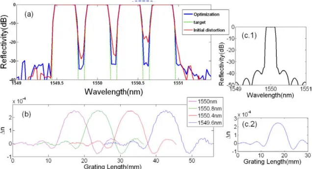
stage moves to the next section...41 Fig. 3 Four-channel FBG filter with 50GHz spacing corrected by the LMO

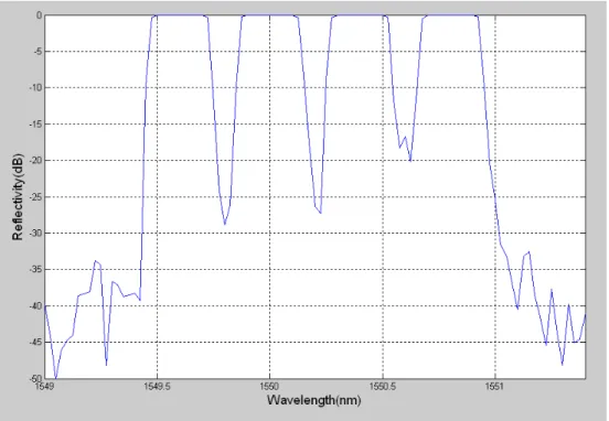
method. (a) Reflection spectra before and after optimization correction to meet the -30dB target. (b) The position distribution and the corrected index modulation. (c.1) The reflection spectrum of each channel without any correction, here is the example of 1550nm channel wavelength. (c.2) The original index modulation of each channel before correction...45 Fig. 3-1 Reflection spectrum of four-channel FBG filter. . ...46 Fig. 3-2 Optimization correction to the target -30dB side-lobe suppression

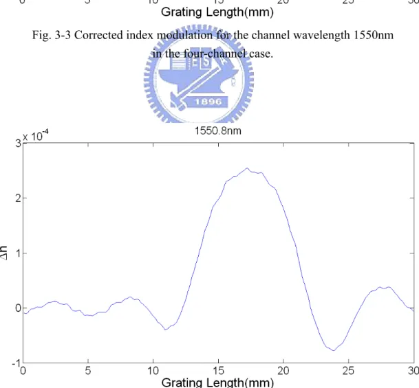
outside the channels by the LMO algorithm. ...46 Fig. 3-3 Corrected index modulation for the channel wavelength 1550nm in

the four-channel case. ...47 Fig. 3-4 Corrected index modulation for the channel wavelength 1550.8nm in

the four-channel case ...47 Fig. 3-5 Corrected index modulation for the channel wavelength 1550.4nm in

the four-channel case ...48 Fig. 3-6 Corrected index modulation for the channel wavelength 1549.6nm in

the four-channel case ...48 Fig. 4 Eight-channel FBG filter with 25GHz spacing corrected by the LMO

method. (a) Reflection spectra before and after optimization correction to meet the -30dB target. (b) The position distribution and the corrected index modulation. (c.1) The reflection spectrum of each channel without any correction, here is the example of 1550nm channel wavelength. (c.2) The original index modulation of each channel before correction...49 Fig. 4-1 Reflection spectrum of eight-channel FBG filter...50 Fig. 4-2 Optimization correction to the target -30dB side-lobe suppression

outside the channels by the LMO algorithm...50 Fig. 4-3 Corrected index modulation for the channel wavelength 1550nm in

the eight-channel case ...51 Fig. 4-4 Corrected index modulation for the channel wavelength 1550.8nm in

the eight-channel case ...51 Fig. 4-5 Corrected index modulation for the channel wavelength 1550.2nm in

the eight-channel case ...52 Fig. 4-6 Corrected index modulation for the channel wavelength 1549.6nm in

Fig. 4-7 Corrected index modulation for the channel wavelength 1550.6nm in the eight-channel case ...53 Fig. 4-8 Corrected index modulation for the channel wavelength 1549.8nm in

the eight-channel case ...53 Fig. 4-9 Corrected index modulation for the channel wavelength 1550.4nm in

the eight-channel case ...54 Fig. 4-10 Corrected index modulation for the channel wavelength 1549.4nm in

the eight-channel case ...54 Fig. 5 The tolerance analyses by the new fabrication method not limited by

the phase mask length. (a) Reflection spectra with ±2%, ±5%, ±10% random errors for the four-channel FBG filter. (b) Reflection spectra with ±2%, ±5%, ±10% random errors for the eight-channel FBG filter ...55 Fig. 5-1 ±2% random errors of the UV beam size and intensity for each scan

step with ±2% random position phase errors in four-channel case...56 Fig. 5-2 ±5% random errors of the UV beam size and intensity for each scan

step with ±2% random position phase errors in four-channel case...56 Fig. 5-3 ±10% random errors of the UV beam size and intensity for each scan

step with ±2% random position phase errors in four-channel case...57 Fig.5-4 Reflection spectra for ±2%, ±5%, ±10% random errors of four-channel

FBG filter. The red line is the original distortion; the black line is ±10% random errors; the blue line is ±5% random errors; the orange line is ±2% random errors and green line is the target reflection spectrum...57 Fig. 5-5 ±2% random errors of the UV beam size and intensity for each scan step

Fig. 5-6 ±5% random errors of the UV beam size and intensity for each scan step with ±2% random position phase errors in eight-channel case...58 Fig. 5-7 ±10% random errors of the UV beam size and intensity for each scan

step with ±2% random position phase errors in eight-channel case ...59 Fig. 5-8 Reflection spectra for ±2%, ±5%, ±10% random errors of

eight-channel FBG filter. The red line is the original distortion; the black line is ±10% random errors; the blue line is ±5% random errors; the orange line is ±2% random errors and green line is the target reflection spectrum ...59

Chapter 1

Introduction

1.1 Multichannel Fiber Bragg grating

Fiber Bragg gratings (FBGs) are essential optical devices in modern optical communication systems and fiber sensor applications where they find their powerful applicability as narrowband filters, dispersion compensators, optical add-drop multiplexers, and laser source tuners, etc [1]. Optical components based on multichannel fiber Bragg grating have recently attracted great interest because their interchannel response facilitates wavelength filtering in dense wavelength-division-multiplexing systems (DWDM) [2,3]. To fabricate multichannel FBGs within limited length of photosensitive fibers, the most simplistic approach is to sequentially superimpose several single-channel FBGs with their location slightly shifted in order to escape the saturation behaviour of the fiber photosensitivity [4]. However, the overlapped single-channel FBGs will still suffer from the spectral response distortion due to spatial and spectral overlap. If the spatial overlapping is wider, in spite of the total length of the multichannel FBG can be shorter, the spectral response distortion will become worse.

Another widely used method for designing and fabricating multichannel FBGs is the sampling method. By encoding a periodic sampling function for the amplitude and/or phase of the seeding single-channel grating, the multichannel reflection spectrum can be generated [5-7]. However, there will still be some interchannel interference, which would cause the distortion in each channel to make channels no longer identical, especially for a strong multichannel grating or when the seeding

grating has steep jumps in either phase or amplitude.

Recently, many inverse design methods or optimization-based approaches for FBG design have been proposed. The advantages of inverse design methods like the inverse scattering discrete layer-peeling (DLP) algorithm are fast, efficient, and direct [8-10]. Nevertheless their designed results would easily exceed the maximum index change of the fiber photosensitivity especially when designing multichannel FBGs. Therefore some optimization-based methods have been used to constrain the maximum index change. These methods include genetic algorithms, Levenberg-Marquardt method, etc [11,12,13]. However, the designed envelopes of the index change for mutichannel FBGs from the optimization-based methods are typically complicated with many sharp index changes and are thus hard to fabricate. Moreover, the required iteration to achieve the optimization may take long time. In the literature there are also reports about using DLP with simulated annealing optimization process to synthesize the multichannel gratings [14].

1.2 Motivation and purpose of the research

In principle, if the distortion of spectrum can be neglected, the superimpose method and sampled method are relatively attractive. The former is the most simplistic approach and the latter is also useful and widely used, particularly because the advanced high index change photosensitive fibers still developing nowadays can accommodate a higher and higher number of channels [15]. In this study, a new optimization correction method for spectral distortion of multichannel FBG design is investigated. The approach starts from some other design methods of multichannel

FBGs especially for the superimpose fabrication method which will suffer from the spectral distortion, and then utilizes the optimization algorithm to correct these distortion. In this work, we will employ the Lagrange multiplier optimization (LMO) algorithm for optimization. The designed examples of superimpose FBGs will be used for demonstrating the correction of spectral distortion, just for the reason of being the most simplistic way for fabrication. Compared with the slow convergence rate of iteration from typical optimization-based methods, this approach can fast and efficiently converge to the optimization target starting from the close initial profile and still retains the easy-fabrication feature. It is especially superior to design higher reflectivity multichannel FBGs because the summation of their profiles may more easily go up to the saturation of the photo-induced refractive index change, where some means are needed to prevent the distortion exceeding the tolerance performance.

After accomplishing the optimization correction, we then investigate a novel fabrication platform and analyze the tolerance of the above multichannel FBG design on such a platform. In the literature, the invention of the phase mask approach made the fabrication of FBG devices easier and stable. However it is more restricted if complicated FBGs are to be made. Therefore, some sequential UV-writing methods have been developed. With a real-time interferometric side-diffraction position monitoring technique, the phase of the FBGs can be controlled precisely [16]. Nevertheless the random phase errors in every UV exposure step still made this method non-accurate than the phase mask method. Other works in the literature fabricate complex grating structures with uniform phase masks based on the moving fiber-scanning beam technique[17]. However, to produce long FBGs needs longer phase masks and the cost of which is more expensive, in proportion to their length and complicated profiles. In this study, a new FBG exposure platform is proposed. Above

the main translation stage of this platform, a smaller translation stage is used and the uniform phase mask is bracket above this smaller one. This design can accomplish writing any length of FBGs by moving the position of phase mask to the next section of writing position, without limited by the phase mask length. For the purpose of period match after moving, the side-diffraction position monitoring is used. By utilizing the reference FBG and the phase mask as the position monitoring components to detect the writing fiber and the phase mask position individually, one can then adjust the PZT to reach period match. This new setup can avoid the requirement of expensive long length of phase masks by using the cheaper way of side-diffraction position monitoring technique to precisely control the phase when the phase mask is moving to the next section.

1.3

Structure of this thesis

The thesis comprises five chapters. Chapter 1 is an introductory chapter consists of an introduction to multichannel fiber Bragg gratings, some general algorithms for multichannel FBG design, motivation and purpose of the research. Chapter 2 describes the background of theories and fabrication methods employed in this research. It contains the coupled-mode theory, transfer matrix method, discrete layer-peeling method, and Lagrange multiplier optimization method. The fabrication methods include sequential UV writing techniques, real-time interferometric side-diffraction position monitoring by probing the reference fiber grating and the phase mask separately, and finally the least square error fitting method for determining the exposure parameters will be introduced. Chapter 3 describes the principles of the

research, the optimization correction of spectral distortion for DWDM multichannel FBG filters and a new fabrication method not limited by the phase mask length will be proposed. Chapter 4 presents the results and discussion of the research. Finally, Chapter 5 gives the conclusions and a discussion of future work.

1.4 References

[1] T. Erdogan, “Fiber grating spectra,” J. Lightwave Technol, Vol. 15, No. 8, pp. 1277-1294, 1997.

[2] X. He, Y. Yu, D. Huang, R. Zhang, W. Liu and S. Jiang, “Spectrum envelope analysis for interleaved sampled gratings with phase-shift,” Opt. Commun, Vol. 281, No. 3, pp. 415-420, 2008.

[3] Y.-G. Han, X. Dong, J. H. Lee, and S. B. Lee, “Wavelength-spacing-tunable multichannel filter incorporating a sampled chirped fiber Bragg grating based on a symmetrical chirp-tuning technique without center wavelength shift,” Optics Letters, Vol. 31, No. 24, pp. 3571-3573, 2006.

[4] Y.-G. Han, X. Dong, C.-S. Kim, M. Y. Jeong, and J. H. Lee, “Flexible all fiber Fabry-Perot filters based on superimposed chirped fiber Bragg gratings with continuous FSR tunability and its application to a multiwavelength fiber laser,” Optics Express, Vol. 15, No. 6, pp. 2921-2926, 2007.

[5] M. Ibsen, M. K. Durkin, M. J. Cole, and R. I. Laming, “Sinc-sampled fiber Bragg gratings for identical multiple wavelength operation,” IEEE Photon. Technol. Lett, Vol. 10, No. 6, pp. 842-844, 1998.

dispersion and dispersion slope compensation,” IEEE Photon. Technol. Lett, Vol. 15, No. 8, pp. 1091-1093, 2003.

[7] X.-H. Zou, W. Pan, B. Luo, M.-Y. Wang, and W.-L. Zhang, “Spectral Talbot effect in sampled fiber Bragg gratings with super-periodic structures,” Optics Express, Vol. 15, No. 14, pp. 8812-8817, 2007.

[8] J. Skaar, L. Wang, and T. Erdogan, “On the synthesis of fiber Bragg gratings by layer peeling,” IEEE J. Quantum Electron, Vol. 37, No. 2, pp. 165-173, 2001. [9] L.-G. Sheu, K.-P. Chuang, and Y. Lai, “Fiber bragg grating dispersion compensator

by single-period overlap-step-scan exposure,” IEEE Photon. Technol. Lett, Vol. 15, No. 7, pp.939-941, 2003.

[10] Y. Ouyang, Y. Sheng, M. Bernier, and G. Paul-Hus, “Iterative Layer-peeling algorithm for designing fiber Bragg gratings with fabrication constraints,” J. Lightwave Technol, Vol. 23, No. 11, pp. 3924- 3930, 2005.

[11] J. Skaar and K. M. Risvik, “A Genetic Algorithm for the Inverse Problem in Synthesis of Fiber Gratings,” J. Lightwave Technol, Vol. 16, No. 10, pp.1928- 1932, 1998.

[12] N. Plougmann and M. Kristensen, “Efficient iterative technique for designing Bragg gratings,” Optics Letters, Vol. 29, No. 1, pp. 23-25, 2004.

[13] C.-L. Lee, R.-K. Lee, and Y.-M. Kao, “Design of multichannel DWDM fiber Bragg grating filters by Lagrange multiplier constrained optimization,” Optics Express, Vol. 14, No. 23, pp.11002-11011, 2006.

[14] H. Li, M. Li, Y. Sheng, and J. E. Rothenberg, “Advances in the Design and Fabrication of High-Channel-Count Fiber Bragg Gratings,” J. Lightwave Technol. Vol. 25, No. 9, pp. 2739 - 2750, 2007.

poly(methyl methacrylate-co-methyl vinyl ketone-cobenzyl methacrylate)-core polymer optical fiber by use of a mercury lamp,” Optics Letters, Vol. 30, No. 10, pp.1117-1119, 2005.

[16] K.-C. Hsu, L.-G. Sheu, K.-P. Chuang, S.-H. Chang and Y. Lai, “Fiber Bragg grating sequential UV-writing method with real-time interferometric side-diffraction position monitoring,” Opt. Express, Vol. 13, No. 10, pp. 3795-3801 ,2005.

[17] W. H. Loh, M. J. Cole, M. N. Zervas, S. Barcelos, and R. I. Laming, “Complex grating structures with uniform phase masks based on the moving fiber-scanning beam technique,” Opt. Letters, Vol. 20, No. 20, pp.2051-2053, 1995.

Chapter 2

Background of the research

2.1

Theories

2.1-1 Coupled-mode theory

Coupled-mode theory is one of the straightforward, intuitive, and reasonably accurate models to describe the optical properties of most fiber gratings. It models the spectral response of a fiber grating given by the corresponding grating structure. Assuming that the fiber is lossless and single mode in the wavelength range of interest, then only one forward and one backward propagation mode need to be considered under the phase matching condition.

Fig. 1 The propagation modes in the general fiber.

In Fig. 1, the total electric field is the superposition of the forward and backward propagation modes E_x(x,y,z)=b₁(z)ψ(x,y)+b_-1(z)ψ(x,y) y) ψ(x, e y) ψ(x, eiβz ₊ -iβz = β=neffk is the propagation constant.

From wave equation: με ₂ 0

2 2 ₌ ∂ ∂ − ∇ x Ex t Er r

thus, 0 t ψ ψ) β y ψ x ψ ( ₂ 2 2 2 2 2 2 2 = ∂ ∂ + − ∂ ∂ + ∂ ∂ _{ω με} => k n (x,y)- }ψ 0 y x { 2 2 2 2 2 2 2 = + ∂ ∂ + ∂ ∂ _β (1) k in here isω με

n , n is the refractive index profile of unperturbed fiber. Equation

(1) is the wave equation in general fibers.

x

Fig. 2 The propagation modes in fiber grating.

Considering the fiber grating in Fig. 2, because there is also the index perturbation in z direction, the wave equation may be written as 2 k2 2( , ,

y x n Ex+ ∇ r z)=0 Thus, [( ) 2 2( , , )] 0 2 2 2 2 2 2 = + ∂ ∂ + ∂ ∂ + ∂ ∂ x E z y x n k z y x (2) ) , , (x y z

n is the refractive index profile of perturbed fiber.

After discussing the wave equation in general fibers and in fiber gratings separately, now considering if one mode is exactly entering the perturbed index such as the fiber grating case in Fig. 3, then the electric field can be written as a superposition of the forward and backward propagating modes near the Bragg wavelength.

x

y) ψ(x, ) ( b y) ψ(x, ) ( ) , , ( _{1 -1} 1 x y z b z z E = +

Put E1 into equation (2), which means E1 satisfies the wave equation in the fiber

grating case. One has

0 ) y) ψ(x, ) ( b y) ψ(x, ) ( )]( , , ( ) [( 2 2 _{1 -1} 2 2 2 2 2 2 = + + ∂ ∂ + ∂ ∂ + ∂ ∂ z z b z y x n k z y x (3)

E1 has to satisfy the equation (1), too. From the equations of (1) and (3) we can obtain

the following equation (4) with ((3)-(b1+b-1)*(1))*ψ(x,y) and integrated over the

xy-plane and by replacing β =n_effk.

0 ) )]( ( 2 [ ) ( 2 _{11 1 1} 1 1 2 2 = + + + + ∂ ∂ − − D z b b b b z β β (4) where

∫

∫

− = dA dA n n n k z D co 2 2 2 2 11 ψ ψ ) ( 2 ) ( (5)

Assume the condition is slowly varying envelope approximation and the phase matching condition. By simplifying equation (4) with setting i z

e

b₁ = β andb₋₁ =e−iβz,

equation (6) can be obtained.

1 11 1 11 1 1 11 1 11 1 ) ( ) ( { b iD b D i dz db b iD b D i dz db − = + + = + − − − − β β (6)

For FBGs, the z-dependence of the index perturbation is approximately quasi-sinusoidal, so ) ( Δ )) ( 2 cos( ) ( Δ _{r,ac r,dc} 2 2 z z z z n n ε π +θ + ε Λ = − ( ) Δ ( ) 2 ) ( Δ r.dc 2 2 ac r, z e e e e z i z _i i z i ε ε π _θ θ π + + = _Λ − _Λ − ₍₇₎

where Λis the grating period.

Put equation (7) into (5) and rewrite D₁₁ as

) ( ) ( ) ( ) ( 2 * 2 11 z z e z e z D κ i z κ i z σ π π + + = Λ − Λ ₍₈₎

The term κ(z) is proportional to ε iθ ac r, e

Δ , which is a slowly varying complex function for ac term. σ(z) is the slowly varying function for dc term.

Let’s now consider more details about b1 and b-1. By neglecting the phase change

from the slowly varying dc term, b1 and b-1 can be rewritten as

z i e z u z b = Λ π ) ( ) ( 1 , z i e z v z b₋ = −Λ π ) ( ) ( 1

Replacing the new b1 ,b-1 terms and substituting equation (8) into equation (6) with

σ(z)=0, one obtains u z q v i dz z dv v z q u i dz z du ) ( ) ; ( ) ( ) ; ( { * + − = + = δ δ δ δ (9)

This equation is the so-called couple-mode equations for FBGs. Here

c n_eff B) (ω ω π β δ = − Λ − = and q(z)=iκ(z), where B B c λ π ω =2 . Furthermore, q(z) here is called the coupling coefficient of the FBG.

2.1-2 Transfer matrix method

According to the coupled-mode theory and Fig4,

Fig. 4 The forward and backward amplitude in FBG.

) 11 ..( ... ... ) ( ) 10 ...( ... ... ) ( { * u z q v i dz dv v z q u i dz du + − = + = δ δ u u q u q v j q qv u j j dz dv z q dz du j dz u d * 2 2 2 2 2 ) | (| ) ( ) ( ) ( δ δ δ δ γ δ + = + + − + = − ≡ = => Assume _γ2 _{= q| |}2 _−δ2 Thus, v dz v d u dz u d 2 2 2 2 2 2 { γ γ = = => ) 13 ...( ... ... ) 12 ....( ... ... { _{z z} z z e v e v v e u e u u γ γ γ γ − − + − − + + = + =

From the equation (10) and (12), one can obtain _± =± − u_± q

j

v γ δ

The boundary condition is v(L)=0, which means v+(L)+v-(L)=0. Thus v(z) can be

simplified by equation (13) to become

z v

z

v( )=2 ₊sinhγ (14)

We also can simplify u(z) by equation (11) and (13) to get ) sinh cosh ( 2 ) ( _{* *} z q j z q v z u = ₊ γ γ + δ γ (15)

If the grating is uniform, then the reflection coefficient is

) sinh( ) cosh( ) sinh( ) 0 ( ) 0 ( ) ( * L i L L q u v r γ δ γ γ γ δ − − = =

and the transmission coefficient becomes ) sinh( ) cosh( ) 0 ( ) ( ) ( L i L u L u t γ δ γ γ γ δ − = =

However, if the grating is nonuniform, it can be thought of being composed with many tiny uniform gratings. So the reflection and transmission coefficient of each tiny uniform grating can be written as the matrix:

⎥ ⎦ ⎤ ⎢ ⎣ ⎡ ⋅ = ⎥ ⎦ ⎤ ⎢ ⎣ ⎡ Δ + Δ + ) ( ) ( ) ( ) ( z v z u T z v z u j (16)

As the result, the whole grating can be described by the total transfer matrix:

⎥ ⎦ ⎤ ⎢ ⎣ ⎡ ⋅ ⎥ ⎦ ⎤ ⎢ ⎣ ⎡ = ⎥ ⎦ ⎤ ⎢ ⎣ ⎡ ⋅ = ⎥ ⎦ ⎤ ⎢ ⎣ ⎡ ⋅ ⋅ ⋅ ⋅ = ⎥ ⎦ ⎤ ⎢ ⎣ ⎡ − ) 0 ( ) 0 ( ) 0 ( ) 0 ( ) 0 ( ) 0 ( ... ) ( ) ( 22 21 12 11 1 2 1 v u T T T T v u T v u T T T T L v L u N N (17)

But how to calculated T ? From equation (14) and (15),

) sinh( 2 ) (z v z v = ₊ γ , ) sinh( ) cosh( ( 2 ) ( _{* *} z q j z q v z u = ₊ γ γ + δ γ => v(z+Δ)=2v₊sinh(γ(z+Δ)) , ) ( sinh( )) ( cosh( ( 2 ) ( +Δ = _{+ *} +Δ + _* z+Δ q j z q v z u γ γ δ γ

Use these equations above, we can find the Tj to fit the matrix (16)

⎥ ⎥ ⎥ ⎥ ⎦ ⎤ ⎢ ⎢ ⎢ ⎢ ⎣ ⎡ Δ − Δ Δ Δ Δ + Δ = ) sinh( ) cosh( ) sinh( ) sinh( ) sinh( ) cosh( * γ γ δ γ γ γ γ γ γ γ δ γ i q q i Tj

When knowing Tj , T can easily be calculated. With the boundary conditions of u(0)=1

and v(L)=0, we can derive

22 21 ) ( T T r δ =− , 22 1 ) ( T t δ = from (17).

2.1-3 Discrete layer-peeling method

The discrete layer-peeling method comes from an inherently discrete model [1]. It was first developed by geophysicists and later be extended by Bruckstein et. al.[2,3]. In the following this discrete layer-peeling method was mainly developed by J. Skaaret. al.[4]. For the Tj previously calculated from the Transfer matrix

method, it can further be thought of composing a pure propagation transfer matrix

Δ

T and a discrete reflector matrix T as illustrated in Fig5. Here Δ is the jρ

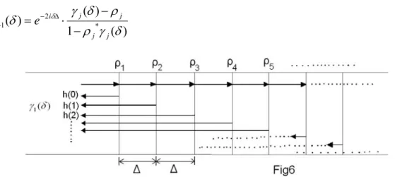
propagation distance and ρj is the j -th discrete reflector.

ρ j j T T T = Δ⋅ ⎥ ⎦ ⎤ ⎢ ⎣ ⎡ = Δ _{− Δ} Δ δ δ i i e e T 0 0 , ⎥ ⎥ ⎦ ⎤ ⎢ ⎢ ⎣ ⎡ − − − = 1 1 | | 1 1 * 2 j j j j T ρ ρ ρ ρ Here | | ) | tanh(| * j j j j q q q Δ − = ρ

Substituting T andΔ T into the (16), we can derive an expression for the reflection _jρ

coefficient γj(δ) Δ + Δ + + + = ≡ _δ δ δ γ ρ δ γ ρ δ δ δ γ i j j i j j j j j e e u v 2 1 * 2 1 ) ( 1 ) ( ) ( ) ( ) ( The equation above can be simplified to

) ( 1 ) ( ) ( 2 _* 1 _{ρ γ δ} ρ δ γ δ γ δ j j j j i j e − − ⋅ = − Δ + (18)

Fig. 6 γ₁(δ) can be thought as the sum of impulse responses from every reflector.

To obtain γ₁(δ) and ρ₁, we first note Fig6. γ₁(δ) can be thought as the sum of impulse responses from every ρjreflector.

∑

∞ = Δ = 0 1( ) ( )exp( 2 ) τ δτ τ δ γ h i (19) In equation (19), Δ = 2 t

τ (t means time), h(τ) is the impulse response for each ρ_j, and )exp(iδτ2Δ is the phase difference caused by every ρ_j. When τ=0, then

) (

1 δ

γ only receive the impulse response from ρ₁.

∫

Δ Δ − Δ = = => 2 2 1 1 1 (0) ( ) π π δ δ γ π ρ h d

The equation above can be expressed as the discrete form:

∑

= = M m m M 1 1 1 ( ) 1 _γ ρ (20) However fiber gratings have limited length. If the grating is thought of being composed with N tiny sections, it is impossible to accomplish equation (19) forτup to

∞ . As the result the apodization-windowing procedure such as the Hanning-window procedure in digital-signal processing needs to be used to confineρto the finite number. Only the ρ in this specific window would be calculated.

The whole steps to realize Discrete layer-peeling method are:

1. Design the target reflection spectrum. γ(δ)and transfer it to a realizable reflection spectrum γ₁(δ) by the Hanning-window procedure.

γ₁(δ)=r(δ)⊗W(δ)

W(δ) is the Fourier transform of w(τ), and

)] 2 cos( 1 [ 2 1 ) (τ = + πτ

w , here⊗means convolution algorithm.

2. Take γ₁(δ) into equation (20) to get ρ₁

3. Substitute ρ₁ and γ₁(δ) into equation (18) to obtain γ₂(δ).

4. Repeat steps 2 and 3 until the whole tiny reflectors ρj are all calculated.

5. Due to | | ) | tanh(| * j j j j q q q Δ − = ρ , so we can get q j ) | | 1 | | 1 ln( 2 1 | | j j j q ρ ρ + − Δ = , argqj =−argρj

2.1-4 Lagrange multiplier optimization method

The method of Lagrange multipliers will be introduced in the following. If we define Λ as the Lagrangian,

∑

+ = Λ k k kg x y y x f y x, , ) ( , ) ( , ) ( λ λ

where f( yx, )is the function to be optimized, gk( yx, )is the constraint functions and

k

λ are the Lagrange multipliers. The optimization realizes when 0 = ∂ Λ ∂ = ∂ Λ ∂ = ∂ Λ ∂ k y x λ

In 2006, Cheng-Ling Lee et. al. applied the Lagrange multiplier constrained optimization method to the multichannel DWDM fiber Bragg grating filters design [5]. Their theory was first starting from the coupled-mode equations.

u z q v i dz dv v z q u i dz du ) ( ) ( { * + − = + = δ δ

Fig. 7 The forward and backward amplitude in FBG.

By the boundary conditions u(0)=1 andv(L)=0and the transfer matrix method, then

) (z

u and v(z) can be obtained.

The design goal is to obtain the coupling coefficient q(z) to produce an output reflection )γ(λ optimally close to the given reflection spectrum γd(λ). We define the objective functional that will be minimized as follows:

∫

∫

∞ ∞ − + − = Φ _d d L q z dz 0 2 2 _{[ ( )]} 2 )] ( ) ( [ 2 1 _{γ λ γ λ λ} β

Here _|2 ) 0 ( ) 0 ( | ) ( u v = λ γ and

∫

L dz z q 0 2 )] ( [ 2 β

is the constraint term for reducing the maximum value of q(z).

Suppose u=u_R +iu_I and v=v_R+iv_I are decomposed into real and imaginary parts.

Substituting them into the coupled-mode equations, we can get: The real part of u Î R + _I − _R =0

qv u dz du _δ

The imaginary part of u Î I − _R − _I =0

qv u dz du _δ

The real part of v Î R − _I − _R =0

qu v dz dv _δ

The imaginary part of v Î I + _R− _I =0

qu v dz dv _δ

So the complete Lagrange Multiplier Optimization functional can be rewritten as:

∫

∫

∞ ∞ − + − = _d d L q z dz J 0 2 2 _{[ ( )]} 2 )] ( [ 2 1 _{γ γ λ λ} β

∫∫

∞ ∞ − − + ∂ ∂ + L R _{I R} R u u qv dzd z u 0 , [ δ ] λ μ ∞

_∫∫

∞ − − − ∂ ∂ + L I _{R I} I u u qv dzd z u 0 , [ δ ] λ μ

∫∫

∞ ∞ − − − ∂ ∂ + L R _{I R} R v v qu dzd z v 0 , [ δ ] λ μ ∞

_∫∫

∞ − − + ∂ ∂ + L I _{R I} I v V qu dzd z v 0 , [ δ ] λ μ

Where μu , μv are the Lagrange multipliers for enforcing u and v to satisfy the

coupled mode equations.

To minimize J, by performing variation to uR, uI, vR, vI, one has:

0 = ∂ ∂ R u J Î ) 22 ..( ... ... ... 0 ) 21 ...( ... ... 0 | )) ( ( 2 1 { , , , 0 , 2 = − − ∂ ∂ − = + − ∂ ∂ q z u R v I u R u L R u d R μ δ μ μ μ λ γ γ 0 = ∂ ∂ I u J Î ) 24 ..( ... ... ... 0 ) 23 ...( ... ... 0 | )) ( ( 2 1 { , , , 0 , 2 = − + ∂ ∂ − = + − ∂ ∂ q z u I v R u I u L I u d I μ δ μ μ μ λ γ γ

0 = ∂ ∂ R v J Î ) 26 ..( ... ... ... 0 ) 25 ...( ... ... 0 | )) ( ( 2 1 { , , , 0 , 2 = − + ∂ ∂ − = + − ∂ ∂ q z v R u I v R v L R v d R μ δ μ μ μ λ γ γ 0 = ∂ ∂ I v J Î ) 28 ..( ... ... ... 0 ) 27 ...( ... ... 0 | )) ( ( 2 1 { , , , 0 , 2 = − − ∂ ∂ − = + − ∂ ∂ q z v I u R v I v L I v d I μ δ μ μ μ λ γ γ

Setting μu =μu,R +iμu,I , μv =μv,R +iμv,I and with the equations (22), (24), (26) and

(28), one has: u v v v u u q i z q i z μ δμ μ μ δμ μ − − = ∂ ∂ − = ∂ ∂ { (29)

To obtain the boundary condition of equations (29), we can focus the other equations (21), (23), (25) and (27). By considering theuR(0) case, with

2 | ) 0 ( ) 0 ( | ) 0 ( u v = γ , from equation (21): 0 ) 0 ( ] [ ) 0 ( 2 1 , 2_{− =} − ∂ ∂ R u d R u γ γ μ 0 ) ( ) 0 ( ] [ ) 0 ( ₂2 2₂ , ₊ = + ∂ ∂ − + − ⇒ I R I R R d R u u u v v u γ γ μ 0 ] ) ( ][ [ 2 ) 0 ( ₂2 ₂2 ₂ , ₊ = + − − − ⇒ I R I R d R R u u u v v u γ γ μ 0 2 ] [ ) 0 ( _{2 2} , − − ₊ = − ⇒ I R R d R u u u u γ γ γ μ (30) Here we only concern the point of z=0.

From equation (23) in the uI(0)case with the similar steps above, one can get:

0 2 ] [ ) 0 ( _{2 2} , − − ₊ = − I R I d I u u u u i iμ γ γ γ (31)

Equations (30) and (31) can be mixed to be simplified to:

2 2 ₍₀₎ ) 0 ( )] 0 ( ) 0 ( )[ 0 ( 2 ) 0 ( ) 0 ( I R d u u u u + − − = γ γ γ μ (32) ) 0 ( v

This means by using the cases of vR(0) and vI(0) with the similar steps above, we can obtain: 2 2 ₍₀₎ ) 0 ( )] 0 ( ) 0 ( [ 2 ) 0 ( ) 0 ( I R d v u u v + − = γ γ μ (33) Finally

∫

∞ ∞ − − − + = ∂ ∂ ) ( ) ( ) ( ) ( [ ) ( ) ( m u,R m R m u,I m I m m z v z z v z z q z q J _{β μ μ} ) 34 .( ... ... ... )] ( ) ( ) ( ) ( _, , μ λ μ_vR z_m u_R z_m − _vI z_m u_I z_m d − q J ∂ ∂

has to be as close to zero as possible.

The whole steps of the optimization algorithm are as follow:

1. Gauss an initial trial qini(z) and let the old function qold(z)=qini(z)

2. Substitute )q_old(z into the transfer matrix method to get u(z)andv(z)from

z=0~L.

3. Once knowing u(0)and v(0), substitute them into the equations (32) and (33) to

obtain the boundary conditions μu(0)and )μv(0 .

4. When knowing μu(0)and )μv(0 , substituting them into equation (29) to obtain

) (z u μ and )μv(z 5. Check ) (z q J ∂ ∂

in the equation (34) to see if it is near zero with the obtained μu(z), )

(z

v

μ ,u(z)andv(z). If not, update q(z) by

) ( ) ( ) ( z q J z q z q old old new _∂ ∂ − = α

where βand α are ad hoc constants. 6. Let qold =qnew, repeat step 2~5 until

q J

∂ ∂

2.2

Fabrication methods

2.2-1 Sequential UV writing techniques

One of the fabrication methods to produce a complex refractive index change fiber grating like in Fig. 8 is the sequential writing technique. By exposing small Gaussian beams of ultraviolet light on the photosensitive fiber step by step as shown in Fig. 8, fiber gratings of complicated refractive index change can be produced. When using the sequential writing technique, the interference pattern must be matched for each step, as illustrated in Fig. 9, so that these small Gaussian ultraviolet beams can be sequentially combined to form a long complex grating. However, this method also arouses an issue: the position errors for each step must be small enough in order to implement complex fiber gratings with high quality.

Fig. 8. A complex refractive index change fiber grating and the sequential writing techniques.

2.2-2 Real-time interferometric side-diffraction position

monitoring by probing the reference fiber grating

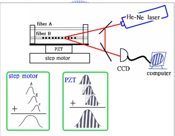
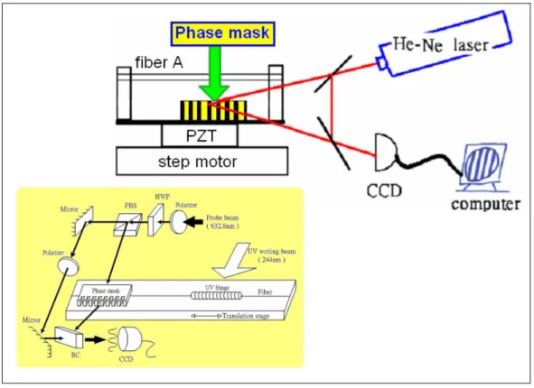
For the sequential writing techniques, the issues of the position errors for each step had been researched by our group. In 2005, we proposed a fiber Bragg grating sequential UV-writing method with real-time interferometric side-diffraction position monitoring to reduce the position errors [6]. Fig. 10 is the easy-looking figure of the previous work. The fabrication platform includes two fibers, one PZT, one step motor, a He-Ne laser for position monitoring, a CCD and a computer for control and data taking. The step motor moves the fiber to other position so that the ultraviolet beam can write on the other position of the photosensitive fiber. On the other hand, the PZT is controlled by the computer for adjusting the phase of interference to match with the phase of the previous step.

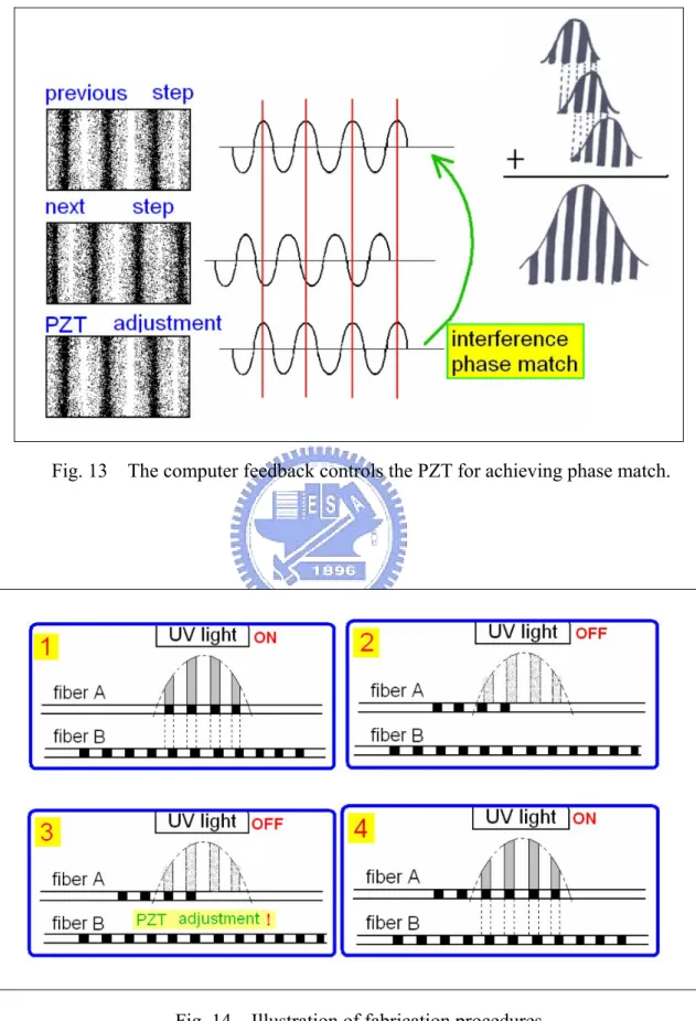
Fiber A is where the ultraviolet light writes. Fiber B is a long reference fiber grating for position monitoring. When the He-Ne laser is incident on the Fiber B, it will diffract into different orders of lights. We use the first order diffraction light to form the interference pattern on the CCD, as shown in Fig. 11. The CCD records the real time interference pattern which contains the position information of the exposed fiber as illustrated in Fig. 12. After the CCD records the real time interference pattern, the computer analyze it, Fourier-transform it into the spectral domain and after filtering it, inverse-Fourier-transform it back to the spatial domain to obtain the phase information. After the computer obtains the phase information of the interference pattern, it will compare with the phase information of the previous step. If the phases between this step and the previous step are not matched, the computer will feedback-controlled the PZT for adjusting until the two phases are matched. In the design, 2% error is acceptable for the feedback control. Fig. 13 is a more simplified

drawing to present the concept. Fig. 14 shows the flow chart of the fabrication procedure. First the ultraviolet light for exposure is turned on. Then the UV light is turned off after exposing one section, the step motor moves the fiber to next position, with possible phase mismatch. The feedback control of PZT adjustment is then achieved by the computer for phase matching. After the phase matching, the ultraviolet light is turned on again for next exposure. The sequential writing can be achieved by repeating the above procedures.

In our previous work,a 58 steps of about 70 mm long Gaussion apodized FBG was produced. The scan step is about 1.2mm. Another example is a 70 steps of 40mm long π-phase-shifted apodize FBG with the scan step about 0.6 mm. These examples demonstrate the feasibility of fabricating phase-shifted fiber gratings by the sequential writing technique. The experimental data are presented in Fig. 15.

2.2-3 Real-time interferometric side-diffraction position

monitoring by probing the reference phase mask

The fabrication platform from our past work still has some disadvantages: First, the Fiber B’s core was too small, making it difficult to align. Besides, the side diffraction efficiency of FBGs was too weak, making the noises from the surrounding become obvious. If the side diffraction efficiency can be larger, the noises can be relatively non-obvious. So the weak diffraction efficiency leads to larger errors for the position monitoring.

The other disadvantage is that the period of the ultraviolet interference light may be mismatched with the reference FBG. Fig. 16 shows how the reference FBG is produced in past work. The CCD reads the interference pattern from the previous step. The reading errors from the previously exposed FBG section may cause accumulative

errors when writing step by step, which means the produced reference FBG will have accumulative errors included.

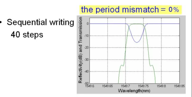
To analyze the effects of the period difference between the position monitoring grating and the ultraviolet interference light, simulation of 40 step sequential writing has been performed as an example. Fig. 17 is the result of 0 percent period mismatch. The side mode suppression ratio of the reflection spectrum is about 35dB. When the period mismatch is 5%, the result is Fig. 18. The reflection spectrum experiences little deformation and a shift of the center wavelength, but is still acceptable. If the period mismatch is larger than 5% , for example, to 10%, the deformation of the reflection spectrum becomes worse and the shift from the center wavelength becomes larger, which makes the quality of the FBG becomes not acceptable for the original design. So the period difference has to be kept lower than 5%.

In 2007, we proposed a new setup of fabrication platform with real-time interferometric side-diffraction position monitoring by probing a reference phase mask [7]. Fig. 19 is the easy-looking figure of the experimental setup. There we used a phase mask as the component for position monitoring to replace the original reference fiber grating. What is the advantage of using the phase mask but not the reference FBG? One of the reasons is that the phase mask component is larger than the small core of the fiber so that it is easier to align. Moreover, the phase mask has diffraction efficiency large to 21%. Compared with the small diffraction efficiency of the reference FBG, the noises from the CCD reading is relatively less-obvious. On the other hand, when the ultraviolet light interference is also made by the phase mask, not the two beam interference, then using the phase mask as the position monitoring can effectively reduce the period mismatch. Also, the phase mask is typically produced by the e-beam method, which may be more accurate than the reference FBG produced by

the sequential writing technique. In our past work, the accumulative errors of the reference FBG may increase the phase errors for every step when using the sequential writing technique. Now, because the less accumulative errors of the phase mask, the phase errors for every step can be reduced.

The reflection and transmission spectra of an apodized FBG fabricated by using this new setup are presented in Fig. 20. Its measured index profile is also shown in the figure. The final FBG is produced after a 40-section sequential writing to yield a total grating length of 40 mm. This demonstrates the feasibility of probing a reference phase mask for position monitoring during the FBG sequential writting.

Fig. 10 The easy-looking figure of the real-time interferometric side-diffraction position monitoring by probing the reference fiber grating.

Fig. 11 The interference setup and pattern on CCD.

Fig. 13 The computer feedback controls the PZT for achieving phase match.

Fig.15 Examples of FBG fabricated.

Fig.17 Result of 0 percent period mismatch between the writing beam and the reference FBG.

Fig. 18 Results of 5 and 10 percent period mismatch between the writing beam and the reference FBG

Fig. 19 Real-time interferometric side-diffraction position monitoring by probing the reference phase mask.

2.2-4 Least square error fitting method for determining the

exposure parameters

In section 2.2-1, the sequential UV writing techniques had been introduced. In order to realize this technique (also called the overlap-step-scan method) for fabricating the designed FBGs [8], we use the least square fitting method [9] to find the best experimental parameters for every sequential exposure steps.

In the overlap-step-scan exposure method, the exposure of every step is a small gaussian beam. Assuming A_m(z) is the refractive index envelope of the m-th small gaussian beam and Aid(z) is the refractive index envelope of the FBG design, then

) (z

A_m can be written as:

) / ) ( exp( ) ( 2 2 ws z z C z A_m = _m⋅ − − _m

Here C is the amplitude of the m-th small gaussian beam, m wsis the width of the

gaussian beam and z is the central position of the m-th exposure gaussian beam. So m

we can determine the optimum parameters of the overlap-step-scan exposure by using the following merit function,

∫

−

∑

= m m id m A z A z dz C }) [ ( ) ( )]2 ({ σ In the above,

∑

m m z

A ( need to be as close to ) A_id(z) as possible. By using the least

square method, this goal can be achieved, if the following equations are satisfied,

∫

−

∑

⋅ − − = − = ∂ ∂ m m m id m dz ws z z z A z A C ) 0 ) ( exp( )] ( ) ( [ 2 2 σ

Therefore, we can get the amplitude of the small gaussian beam for each step in the sequential UV writing technique by solving the above set of linear algebraic equations for C with given m ws and z . m

2.3 References

[1] R. Feced, M. N. Zervas, and M. A. Muriel, “An efficient inverse scattering algorithm for the design of nonuniform fiber Bragg gratings,” IEEE J. Quantum Electron, vol. 35, No. 8, pp. 1105-1115, 1999.

[2] A. M. Bruckstein and T. Kailath, “Inverse scattering for discrete transmission-line models,” SIAM Rev, vol. 29, No. 3, pp. 359-389, 1987.

[3] A. M. Bruckstein, B. C. Levy and T. Kailath, “Differential methods in inverse scattering,” SIAM J. Appl. Math, vol. 45, No. 2, pp. 312-335, 1985.

[4] J. Skaar, L. Wang, and T. Erdogan, “On the synthesis of fiber Bragg gratings by layer peeling,” IEEE J. Quantum Electron, vol. 37, No. 2, pp.165-173, 2001.

[5] C.-L. Lee, R.-K. Lee , and Y.-M. Kao, “Design of multichannel DWDM fiber Bragg grating filters by Lagrange multiplier constrained optimization,” Optics Express, Vol. 14, No. 23, pp.11002-11011, 2006.

[6] K.-C. Hsu, L.-G. Sheu, K.-P. Chuang, S.-H. Chang and Y. Lai, “Fiber Bragg grating sequential UV-writing method with real-time interferometric side-diffraction position monitoring,” Opt. Express, Vol. 13, No. 10, pp. 3795-3801, 2005.

[7] K.-C. Hsu, C.-W. Hsin, T.-H. Yen, and Y. Lai, “Fiber Bragg grating sequential writing method by real-time probing a reference phase mask,” Fibers and Optical Passive Components International Conference, W3A-5, 2007.

[8] L.-G. Sheu, K.-P. Chuang, and Y. Lai, “Fiber Bragg Grating Dispersion Compensator by Single-Period Overlap-Step-Scan Exposure,” IEEE Photon. Technol. Lett, Vol. 15, No. 7, pp. 939-941, 2003.

[9] W. H. Press, S. A. Teukolsky, W. T. Vetterling, and B. P. Flannery, Numerical Recipes in C (Cambridge University Press, New York, 1992).

Chapter 3

Principles of the research

3.1 LMO algorithm for optimization correction of

superimposed FBG design

In this study, we adopt a hybrid approach which mixes the Lagrange multiplier optimization (LMO) method with other algorithms for the case of superimposed fabrication method. The LMO algorithm starts from the following objective functional that needs to be minimized:

∫

−∞∞ − = γ λ γ λ dλ J [ ( ) _d( )]2 2 1

∫ ∫

−∞∞ ∂ + − ∂ + L R I R R R R qS dzd z R 0 μ , [ δ ] λ

∫ ∫

−∞∞ ∂ − − ∂ + L I R I I R R qS dzd z R 0 μ , [ δ ] λ

∫ ∫

−∞∞ ∂ − − ∂ + L R I R R S S qR dzd z S 0 μ , [ δ ] λ

_{∫ ∫}

∞ ∞ − ∂ + − ∂ + L I R I I S S qR dzd z S 0 μ , [ δ ] λ (1)

Here _{γ(λ)=|S(0)/R(0)|}2 _{is the FBG reflection spectrum which is determined by}

the coupling coefficient q. The design goal is to minimize the difference of γ(λ) and

the target reflection spectrum γ_d(λ) by setting ∂J/∂R=∂J/∂S =0 and iterative calculating ∂ /J ∂q_j till it converges to zero. In this equation the Lagrange multipliers

are separated into real and imaginary parts, μ_R =μ_R,R+iμ_R,I and μ_S =μ_S,R+iμ_S,I. On

the other hand, in order to simulate different periods of gratings superimposed with each other, the period shift from λ_D (λ_D =2n_effΛ, Λ is the grating period) can be

thought as the linear phase shift of the coupling coefficient. As the result, the coupling coefficient for each exposure can be written as

) 2 sin 2 )(cos ( ) 2 exp( ) (z i z q z z i z

q_j −_lj ⋅ δ_j ≡ _j −_lj δ_j + δ_j . Here _lj is the position shift for

avoiding the index change saturation of the photosensitivefiber, and λ λ π δ =−2 ₂ ×Δ D eff n . We apply the discrete layer-peeling method to synthesize the initial coupling coefficient for each single channel and therefore the obtained q_j(z−_lj) are real in this study.

In the case of the superimposed fabrication method, the total length L could be composed of several parts. For example, we can consider three different periods of gratings superimposed to form the total length L, as shown in Fig. 1. Then the total length of FBG should be divided into five sections: 0~L1, L1~L2, L2~L3, L3~L4, L4~L.

The corresponding coupling coefficients are q₁ , q₁+q₂⋅exp(2iδ₂z) ,

) 2 exp( ) 2 exp( _{2 3 3} 2 1 q i z q i z

q + ⋅ δ + ⋅ δ , q2⋅exp(2iδ2z)+q3⋅exp(2iδ3z) , q3⋅exp(2iδ3z)

respectively.

Fig. 1 Example of three channel superimposing.

To minimize the cost function J, variation with respect to the forward- and

backward modes Rand S is used and the equations of the corresponding Lagrange

multipliers become,

{

R S S S R R q i z q i z μ δμ μ μ δμ μ − − = ∂ ∂ − = ∂ ∂ (2)

In Eq(2), q needs to be replaced by different coupling coefficients of different

sections such as the five sections in the example above. The boundary conditions of Eq(2) could be obtained by varying R and S at z=0,

2 2 ₍₀₎ ) 0 ( )] 0 ( ) 0 ( )[ 0 ( 2 ) 0 ( ) 0 ( I R d R R R R + − − = γ γ γ μ 2 2 ₍₀₎ ) 0 ( )] 0 ( ) 0 ( [ 2 ) 0 ( ) 0 ( I R d S R R S + − ⋅ = γ γ μ (3) Afterwards, the cost functional J is varied with respect to the coupling

coefficient q_j to obtain:

∫ ∫

−∞∞ − − − − = ∂ ∂ 1 0 . , , , 1 ] [ L I I S R R S I I R R R R S S R R dzd q J _{μ μ μ μ λ}

∫ ∫

−∞∞ − ⋅ − ⋅ = ∂ ∂ j j L L RR I j R j j z i S z i S q J 1 )) 2 cos( ) 2 sin( ( [μ _, δ δ )) 2 cos( ) 2 sin( ( ,I SR i jz SI i jz R δ δ μ ⋅ + ⋅ − )) 2 sin( ) 2 cos( ( ,R RR i jz RI i jz S δ δ μ ⋅ + ⋅ − λ δ δ μ_S,I(R_R⋅sin(2i _jz)−R_I ⋅cos(2i _jz))]dzd + (4) The whole LMO algorithm mixed with the superimposed method may be summarized in the following:

1) After getting the coupling coefficient q_{j_ini} by the discrete layer-peeling method,

superimpose them and calculate the distortion of reflection spectra. Let ) ( ) ( _{_} _ z q z q_{j old} = _{j ini} .

2) From the coupled-mode equations with the q_{j_old} getting from step 1), R(z) and

) (z

S can be obtained from z=L to z=0.

3) Use Eq(3) to set the boundary conditions of μ_R(0) and μ_S(0). Then use Eq(2) to calculate the Lagrange-multiplier functions μ_R(z) and μ_S(z) from z=0 to

L

4) Find ∂ /J ∂q_j by Eq(4). If convergence is not reached, update the coupling coefficients by j old j new j q J z q z q ∂ ∂ − = ( ) α ) ( _{_} _

where α is an ad hoc constant, which can determine the iteration rate. 5) Let q_{j_old} =q_{j_new} and repeat the steps 2) to 4) till ∂ /J ∂q_j converges to zero.

3.2 A new fabrication method not limited by the phase

mask length

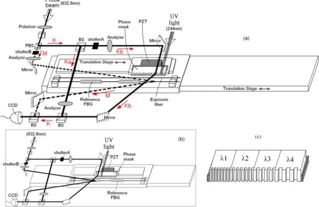
In this section we present a new FBG fabrication platform that is not limited by the length of the phase mask. In Fig. 2(a), the function of the based translation stage is to move the writing fiber to different position for exposing UV lights. A smaller translation stage mounted on it is to move the uniform phase mask fixed above the smaller translation stage. When the writing module has written the length of FBG nearly equals to the phase mask length, the smaller translation stage can be used to extend the writing range. Other components in the setup include a writing fiber, a reference FBG that is made by this uniform phase mask is for side-diffraction position monitoring and a piezoelectric translator stage (PZT) which is between the smaller translation stage and the uniform phase mask with sub-nm position resolution for accurately fine-tuning. Further in Fig. 2(a) it also shows a He-Ne laser (632.8nm) for probing the position information. The laser beam is divided into two probe beams K and M with a polarization beam splitter. The probe beam M will emit into the reference FBG and generate the diffraction beams. The probe beam K splits again into two probe beams Ka and Kb. Kb will emit to the phase mask and the diffraction beams will be generated, too. Ka functions as the reference beam to form the interference pattern with the diffraction beams from Kb or M for obtaining the phase information with the CCD camera connected to the computer.

When the UV light is exposing the writing fiber of which the length still not exceeds the phase mask length, the shutterB closes, and the shutterA opens. The interference pattern read by the CCD camera is produced with the probe beams Kb and Ka, which carries the phase information of the phase mask. Therefore when the phase shift is required by the design of FBG, the computer can analyze this phase

information from the CCD and then controls the PZT for fine-tuning the phase mask position to produce the phase shift.

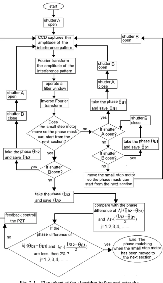
However, if the UV lights have been exposing the writing fiber of which the length nearly exceeds the phase mask length and will continue exposing to longer length, the small translation stage will start to move the PZT stage with the phase mask mounted on it to the next written section, as shown in Fig. 2(b). In this figure, the base translation stage moves rightwards so that the phase mask is now probed in its left end. At this time, the smaller translation stage will be ready to move leftwards for the next writing section. However, in order for the UV interference phase can match with that of previous section after moving, the computer should record the phase of previous section and control the PZT for fine-tuning to match the phase with the previous one. Further, since the adjacent FBG sections have to be joined with high accuracy, the mechanical vibration errors during the movement of the smaller translation stage should also be concerned because it may cause the phase shift errors between the writing fiber and the phase mask. We utilize a reference fiber Bragg grating to probe this movement error. Since the writing fiber and the reference FBG are mounted on the same base translation stage, not the smaller translation stage, thus by probing the reference FBG one can acquire the writing fiber position shift information from the phase change of interference read by the CCD. In short, the section-by-section connection moment of the phase mask moved by the smaller translation stage may be summarized in the following steps:

1) Close the shutterB, open the shutterA, then the CCD records the interference phase information θ_a1 for the phase mask.

2) Close the shutterA, open the shutterB, then the CCD records the interference phase information θ_b1 for the reference FBG.