ACTIVE CONTROL OF AN ASYMMETRICAL RIGID ROTOR SUPPORTED BY MAGNETIC BEARINGS

Active Control

of

an Agmmetrical Rigid

Rotor Supported by Magnetic Bearings

Department of Mechanical Engineering, National Chiao Tung University,

1001 Tu Hsueh Road, Hsinchu 30049, R.O.C.

ABSTRACT : Vibration control of a horizontal rotor with an asymmetrical moment of inertia is investigated. A linear optimal control system is developed to stabilize and control the rotor

system by using the mathematical model of a rotor system expressed in the rotating

coordinates. An approximated dynamical equation of a long rotor system is derived and used

to obtain the compensator in analytical ,form (which saves much computational effort in

control design), and is particularly useful in hardware implementation. Simulation results

show the eficiency of the proposed strategy. The influences of weighting matrices and the

eflects of the asymmetrical moment of inertia on system performance,for dtfferent controllers

are also assessed.

I. Introduction

The dynamics of asymmetrical rotor systems has received a great deal of attention in recent years, but how to control these rotor systems has not been studied in great detail. A few papers have discussed the stability analysis of an asymmetrical rotor-bearing system (l-7), and the vibration control problem of symmetrical rotor-bearing systems (S-15), but little has been reported about the vibration control of an asymmetrical rotor-bearing system (16). For example, Matsumura

et al. (8) considered a horizontal rotating shaft controlled by magnetic bearings.

They derived the equations of motion of a levitated rotating body, made clear the relations between voltage, current and attractive force of an attractive-force-type electromagnet and showed that an integral controller is desirable. Anton and Ulbrich (16) considered the effect of asymmetries on a high-speed rotor where an output feedback control was designed based upon the symmetric part (i.e. time- invariance matrices) of the rotor system, whereas the unsymmetrical part was omitted from their account. The method, though simple, does not warrant the stability of the controlled system, which in reality depends heavily on the influence of asymmetries. Furthermore, neglect of the unsymmetrical part in the control design may deteriorate the system performance even if the controlled system is stable.

This paper is concerned with the active vibration control of an asymmetrical rigid rotor system. All the degrees of freedom of motion, except the translation

Yi-Hua Fan et al.

motion in the axial direction and the rotation of the spin motion, are actively controlled by the attractive forces which are provided by the direct current electro- magnets. Taking into account the effect of the asymmetrical moment of inertia, the motion equations of the rotor system consisting of periodic coefficients are first developed. Then, for the purpose of convenience in control design, these equations are readily transformed into a rotating coordinate system in which linear constant- coefficient differential equations are obtained. Based on these equations, an optimal control system is then developed to suppress the vibrations of such an asymmetrical rotor system.

Because of the complexity in solving the Riccati equations, an analytical form of the solution (if considering a long rotor system) is further developed in this paper. Mizuno and Higuchi (9) utilized the concept of the internal symmetry of a system to obtain the solution of this problem. Unfortunately, the appearance of the unsymmetrical moment of inertia makes this available concept useless. To overcome such difficulty, an approximated model suitable for a long rotor system is derived. The concept of the internal symmetry of system, based on this new approximated model, can still be used to develop an analytical form of the optimal control problem. This saves much computational effort in control design and is most useful for hardware implementation or analog control. Simulation results have shown the efficiency of this proposed strategy.

It. Modeling

qf

The rotor is assumed to be rigid and asymmetric, in which, for easy modeling, the cross-section of the shaft is considered to be elliptic with uniform mass imbal- ance. For the general cases where rotors have different moment of inertia properties in the mutual perpendicular planes, the treatment here can still be applied in a similar way. The shaft is suspended horizontally by contact-free magnetic bearings at both ends and rotates at a constant angular velocity Q. as shown in Fig. I. The rotor has four degrees of freedom including two translational motions and two rotational motions, and is controlled by eight magnetic bearings. Figure 1 also shows the direction and point of action of each force.

2.1. The rotuting coordinate system with Eulerian angles

To derive the equations of motion, we first define the Eulerian angles as three successive rotations, which are utilized to describe the angular displacements. As shown in Fig. 2, the sequence employed here is begun by rotating the initial system of axes parallel to the fixed coordinates into deflected mode by an angle 4 counterclockwise about the Z-axis. In the second stage, the intermediate axes (XYZ)’ rotated about the X’ axis counterclockwise by an angle 8 to other inter- mediate axes (UVW)‘. Finally, the (UVW)’ axes are rotated by an angle $ about the W’-axis to produce the principal axes UVW. Eulerian angles 4, H and $ thus completely specify the orientation of the principal coordinate system relative to the fixed coordinate system. The angular velocities are directly described in (UVW)’ as

1154

Journal of the Franklm lnst~tute Pergamon Press Ltd

Control of a Rigid Rotor

electromagnets b

ic->

Cross section of the shaft FIG. 1. Basic structure of the rotor-bearing system.

u; =

B

01;. = fJ sin 0

o:,. = $+d cos 8. ₍₁₎

Then the components of the angular velocities in the directions of the principal axes are individually derived by coordinates transformation, or

0, =8cos$+dsinOsin* 0,. = -8sin$+$sinfIcos*

w, = ~+b;cosd. ₍₂₎

When a rotor element is deflected in position and orientation, the deflected angles are obtained by projecting the inclination angle 8 onto the YZ and XZ planes, as shown in Fig. 2, i.e. 8, = 19 cos 4, O? = 8 sin 4. From the geometric configuration with very small oblique angle 0, the spin angle of rotor about the axis W is obtained as @ = 4+$. Thus, the speed of spin rotation is Q = 6.

2.2. Equations of motion

The dynamic equations of an asymmetric rotor system can be derived through Hamilton’s principle, which states that the actual path renders the integral between two fixed time bounds as shown in Eq. (3) an extremum :

H=

s ‘I 12[(T-P)+ W]dt, (3)

where T, P and W are the kinetic, potential energies and work done by non- conservative forces.

Vol. 329, No. 6, pp. 1153-I 178, 1992

Yi-Hua Fun et al.

(a) Euler angles of the element

(b) Projection of the element

FIG. 2.

t[m(a’+3L)+(I,,~~+Z,.~,Z+Jl,0~.)]. (4)

Substituting Eqs (2), 0, = 8 cos 4, 8, = 8 sin c$, @ = ~+I/I and CI = d+ 4 into Eq. (4) and letting cos 0 = I- (O’j2) and sin 8 = 0 (since 8 is very small), we obtain the total kinetic energy of the rotor as follows :

T = $[m(ii-’ +jZ)+1,1~2 +Z$(d,f?,.-&O,) +I(ti,‘+d;)

+ 2Ag,d,. sin 2D + A(@ - 6;) cos 201, (5) where I and A denote the mean and the deviatoric mass moment of inertia in the principal axes, respectively, i.e.

1156

Journal ol-the Frankhn lnst~tute Pergamon Press Ltd

Control of a Rigid Rotor

I=

l(Zu+Z,.)

A = + (I,, -I(,). (6)

Since the rotor is considered to be rigid and horizontally suspended, the potential energy is influenced by the conservative force of gravity. The total potential energy can be expressed as

P = mgy. (7)

The imbalance force of the rotor during rotation is derived as dF,, = ~0~ dm

dF,. = CR’ dm, (8)

where E and [ are the mass eccentricity components of the shaft corresponding to the axes U and V.

They can be transformed into the fixed coordinates by

dF,

1 [

I[ 1

cos

&CF

=

_{I[ 1}

The work done by distributed imbalance forces is integrated along the rotor and obtained as

Then, by using Eq. (3) the equations of motion can be obtained as follows :

m,i! = m(sQ* cos Qt - CR’ sin fit) + F, - F3 + FS - F7

mj=m(cR’sinRt+jQ’cosRt)-mg+F,-F4+F6-F8

(I- A cos 2Qt)gv + A sin 2Qt& + 2RA sin 2flt8,. - ll(Z, -2A cos 2!Zt)6, = g(-F,+F,+F,-F,) (I+ A cos 2Qt)flv +A sin 2Qt[, - 2QA sin 2Rt4, +fi(I, + 24 cos 2Qt)d)

= ;(F2-F,-F,+F,). (11)

Considering the characteristics of the electromagnets, the input forces F, to F8

can be represented as

F = kdg+k,i, ₍₁₂₎

Vol. 329. No 6, pp. 1153-l 178. 1992

Yi-Hua Fan et al.

where kd is the forceedisplacement factor, k, is the force-current factor, g is the displacement of the magnet gap and i is the incremental current of magnet ~1.

For the sake of simplicity, we assume that the eight electromagnets have the same coefficients kd and k,. Then the eight input forces can be written as :

F3 = k,i;+kd( -x+ 58,)

F4 = kiid+k,(-y- fH,)

Fx = k,i,+k,( -y+ gQ.v). (13)

Substituting these control forces (13) into Eq. (1 l), we obtain the dynamics of the rotor-bearing system as follows :

m?-4kdx = PZ(&’ cos !2-jO’sin Qt)+ki(i, --ij -t-i5 -i,) w+4kdy = m(cR sinRr+@ cos!%)-mg+k,(i2-ii,+i,-i,)

(I-A cos 2flf)oV+A sin 2Ote,.+2QA sin 2&d,.-O(Z, -2A cos 2Cb)8, - L2kdd,. Lk,

= 2-(-il+i3+is-i7) (Z+A cos 2Qr)8, +A sin 2!&tV-2flA sin 2Rtd,, +Q(Z,+2A cos 2Qt)8,.-L’k,O,

= +(i:_i,-i,+i,). (14)

III. Coordinate Transformation and Control Design

Since the coefficients of the equations of motion in the fixed coordinate system are time-varying and complicated, for ease of control design, a special coordinate

1158

Journal of the Frankhn Institute Pcrgmon Press Ltd

Control of a Rigid Rotor transformation is used to simplify the equations of motion. By considering a Cartesian-coordinate system o-uvz which rotates about the z-axis with an angular velocity of Q and assuming that the u-axis coincides with the x-axis at t = 0, we have the following relationships between the coordinates x, y, 6,X and O,,. and the coordinates u, v, 0, and 8, :

x=ucosQt-vsinat J’= usinRt+vcosRt 0, = 0, cos 0th8,, sin Qt

0, = 8,‘ sin Cl+O, cos Cit. ₍₁₅₎

The substitution of Eq. (15) into Eq. (14) yields the equations of motion (16) in the rotating coordinate system where the coefficients are time invariant and simpler than those in the fixed coordinate system. The following differential equations are obtained with respect to u, v, 8, and 0,. :

ii-2Qti-((R2+4k,,)u=BR2-gsinnt+:(U,-U,+U,--U,)

d+2flti-(R2+4kd)v = [R2-gcosQt+;(U2-&+a,-U,)

(Z-A)~~.+~(2Z-Z~)~,+[~‘(Z~-A-Z)-k,L2]~,.=~(-U,+U,+U,-U7),

(16) whereU,,i= I,..., 8 denotes the virtual currents in the rotating coordinates, and is expressed by

[

Ul

us us

u7

U2 U4 U6 _{Us 1} =

_[

From the equations of motion (16), we find the system can be isolated as two subsystems; one subsystem consists of two translational motions and the other comprises two rotational motions. It means that the controller can be separated into two parts; one controls the subsystem of two translational motions and the other controls one of the two rotational motions.

The subsystem of the two translational motions can be represented as

where

k,(t) = A,X,(t)+B,U,(t)+F,W,(O, (18)

Vol. 329, No. 6, pp. 1153-l 178. 1992

Yi-Hua Fun et al. X,=[u u 2’ ti]’ 0 1 0 0 A R’+4& 0 0 2Q , = 0 0 0 1 0 -2fl R2+4kd 0

~I-~1+~5-~7

U*-U4+Uh-U8

1

rooo1 ^

B,=

klm

0

Similarly, the subsystem of the two rotational motions can be represented as

%(r) =

&f,(f) +

BrUr(f),

U*-U4-Uh+UX

1

The object of controller design is using the magnetic bearings to hold the rotating shaft as close as possible to a fixed position, i.e. x = 0, y = 0, 0, = 0 and eY = 0. In other words, if the rotor is perturbed from the equilibrium position by any disturbance (e.g. imbalance forces), the action of the controller will rapidly tend to reduce the deviations. Also, it is reasonable to ask the control forces be kept as small as possible. To meet these requirements, we will design the controller by utilizing linear quadratic regulator theory.

1160

Journal of the Franklin lnst~tute Pergamon Press Ltd

Control of a Rigid Rotor

First, we consider the subsystem of translational motion. Since the magnetic bearing can provide an initial bias force to counteract the weight of the rotor, we can represent the input currents as

i, -i3+i5-i7 = i:(t)-i:(t)+i:(t)-i:(t)

i2 - i4 + ih - i8 = ito + i& + i:(t) - i:(t) + i:(t) -i;(t), (20)

where i&, = i& = m2g/2k, (bias currents) and if(t) is the incremental current of the magnet j.

By Eq. (17), we get

u, = u,-u,+u/i-u,

=mgsinnt+UT-UT-/-UT-U: lA2 = uz-uq+ujb-u8

= mg cos lbl- U:- UT-I- Ub- U$, (21)

where U,* represents a virtual incremental current in the rotating coordinates. Then Eq. (18) can be rewritten as follows :

J&(t) = A,X,(t)+B,U:(t)+F:W:(t), (22)

where

u:: =

u:

u:.

UT-

u:+

=

u:-u;+u;-u;

I

I

J, =

s 0 r (XfQX,+ U:TRU::)dt,

1

w: =

[cl’].

Gic cost function

(23) where Q and R are the weighting matrices, which are selected as

Q = diag (pI,p2,p1,pd,

pl 3 0 and p2 3 0

and

R = diag (1, 1).

The optimal feedback gain K, and input UT are obtained by solving the following algebraic Riccati equations

P,A, + A:P, - P,B,R ’ B,?P, + Q = 0. ₍₂₄₎

In consequence, we obtain K, = - Rp ‘BTP, and UT = K,X,(t) for any initial con- dition X,(O) = X,,.

Secondly, let us look at the subsystem of the rotational motion. Since there is no disturbance appearing in this subsystem, according to Eq. (19) the control force

U, is selected to minimize the quadratic cost function : Vol. 329, No. 6, pp. 1153-I 178. 1992

Yi-Hua Fan et al.

Jr = s

x (X,‘QX, + U,TRUr) dt, (25)

0

where Q and R are the weighting matrices and selected as before.

The optimal feedback gain Kr and input U, are also obtained by solving the following algebraic Riccati equations

P,A,+A,TP,-P,B,Rp’B,TP,+Q = 0. (26)

Similarly, we can get K, = -R ’ BTP,. and (i, = K,.X,(t) for any initial condition X,(O) = x,0.

For both subsystems, since (A,, B,) and (A,, B,) are controllable and (A,, H) and (A,, H) are observable for any H which satisfies HTH = Q. Eqs (24) and (26), respectively, have the unique symmetric positive definite solution P, and P,; and the closed-loop subsystems described by

2, = (A,-B,R-‘BTP,)X, and yr = (A,-B,R -‘BIP,)X, (27) are stable.

In most cases, the solution of the Riccati equations can only be found by numerical computations. Tn this study, following the design procedure presented by Mizuno and Higuchi (9), we find the Riccati equations of the controlled sub- system of translations can still have an analytical solution, as presented in Appendix A. Figures 3 and 4 give the block diagrams of the two optimal regulator subsystems.

The subsystem of translational motion

L-_-_---J

Optimal feedback controller

FIG. 3. The block diagram of the optimal translational regulator subsystem

1162

Journal of the Franklm lnst~tute Pcrgamon Press Ltd

Control oj’a Rigid Rotor

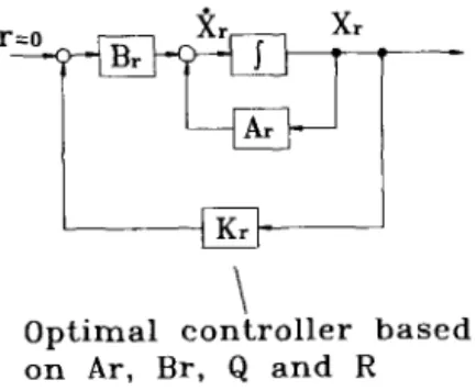
Optimal controller based on Ar, Br, Q and R

FIG. 4. The block diagram of the optimal rotational regulator subsystem.

3.3. Approximate controller design for the rotational subsystem

For most rotor systems, the longitude of shaft is always larger than its radius. If we assume that L2 >> a2 and L2 >> b’ (L is the length of shaft, a and b are semi- major and semi-minor axes of the ellipse cross-section of the shaft), from Eq. (6), we have

,,,=,.=~f;+-r’=‘;:’

(,-A&I=

-~+?$_~

Substituting the above equations into Eq. (19), we obtain yr;(t> = AX,(t) +&U,(t), where

0 0

0 2Q

0 1

-20 R*+12k,/m 0

The algebraic Riccati equations (26) become

(28)

(29)

Vol. 329. No. 6, pp. 1153-I 178, 1992

Yi-Hua Fun et al.

The subsystem of the rotational motion

1 sa_b(I-A+I,)+hL* I+A r=O

+

I

IT+ IzYP~~fq ! j

Fro. 5. The block diagram of the approximate optimal rotational regulator subsystem.

P,,A,,+A:P,,-P,,B,,R~‘B:P,,+Q = 0. (30)

Since the matrices A,,, B,,, Q and R also satisfy the condition J4 ‘A,J4 = A,, J4 ’ B,J2 = B,, JiQJ4 = Q and J$RJ, = R, similar to the procedure in Appendix A, the analytical solution P, can be obtained, and K,, = -R- ‘BTP,, and CJr = K,,X,.(t). The solution procedure of P,, is presented in detail in Appendix B. Figure 5 gives the block diagram of the approximate control subsystem.

IV. Simulation Results

Simulations are based on the rotor system shown in Fig. 1, and details are listed in Table I. In this study, the angular velocity of shaft is assumed to be C2 = 1000 rad/sec and disturbances come only from imbalanced forces. The behavior of the open-loop system is firstly observed. From Eqs (18) and (19), the characteristic values of A, and A, are shown in Table 11 in which the positive characteristic values indicate that the rotor-bearing system is initially unstable. Therefore, an active controller is required to stabilize such a system.

4.1. The responses qf’thc optimal regulutor system

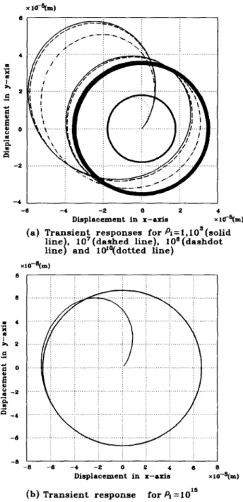
(a) The translutionul subsystem. Figures 6 and 7 show the responses of the translational subsystem to the initial condition X,(O) = [0 0 0 OIT; Fig. 6

1164

Journal of the Franklm lnstitutc Pergamon Press Ltd

Control oJ’a Rigid Rotor TABLE I

Geometric und material properties qf’the rotor system

Density of the shaft material Total length of the shaft

Radius of the ellipse cross-section

7750 kg/m3 L = 0.6 m

u = 0.030 m b = 0.028 m Mass eccentricity components of the shaft

corresponding to axes U and V E = 0.0003 m ( = 0.0003 m Force-displacement factor k, 5.6 x lo5 N/m

Force-current factor k, 250 N/A

shows the case where p, changes from 1 to 10” while pz is fixed to I ; Fig. 7 shows the case where p, is fixed to 1 and pz changes from 1 to 10’ ‘. It is observed that the former has better performance, i.e. shorter settling time and lower contracting radius than the latter.

These phenomena can be explained from the root loci of the controlled sub- system. Figure 8 shows the root loci of the subsystem of the translational motions. Figure S(a) describes the case where p, changes from 1, 10 to 10’ 5 and pz = 1. Figure S(b) describes the case where p, = 1 and p2 changes from 1, 10 to 1015. As listed in Table I, it is observed that the open-loop subsystem is initially unstable. Now considering the effect of control action where p, = 1 and p2 = 1, the closed- loop subsystem is immediately stabilized by shifting the unstable poles to (- 383 k 7921’). Further, when either weighting coefficient p, or p2 is fixed to 1 and the other changes from 1 to IO’, the closed-loop poles are almost the same as those in the case of p, = 1 and pz = 1. However, when the weighting coefficient increases from 10’ to 1015, the closed-loop poles in Fig. S(a) move toward (- 60,000, +60,000) and the closed-loop poles in Fig. 8(b) move toward (- 6e-t 9, f 2e + 6) and (0,O). Physically, the damping ratio and the magnitude of stiffness will increase when the weighting coefficient p, is increasing; but, when the weighting coefficient pz is increasing, the magnitude of stiffness will decrease.

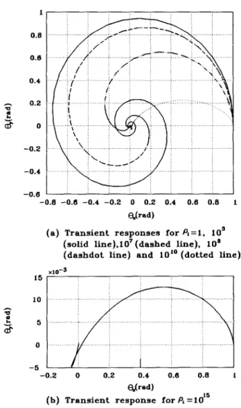
(b) The rotation& suh.~~~stenz. Figures 9 and 10 show the transient responses of

the rotational subsystem to the initial condition X,.(O) = [l 0 0 O]r; Fig. 9

TABLETI

The churacteristic culues qf’ the open-loop system

Subsystem of translational motion Subsystem of rotational motion l.Oe+3 x -0.425 + 1 .OOOi -0.425 - 1 .OOOi 0.425 + 1 .OOOi 0.425 - 1 .OOOi l.Oe+2 x - 1.321+ 9.9301’ -7.327-9.9301’ 7.327+9.9301 7.327 - 9.9301’

Vol. 329, No. 6. pp. 1153-I 178. 1992

Yi-Hua Fan et al. ‘.... :

,.

,

Ml

i

(a) Transient responses for 4=l,lO”(solid

lO’(dashed line). lO’(dashdot

and ld0(dotted line)

x10-q(m) 6 6 -6 -6 -2 -2 -4 -2 cl 2 4 2 2

Displacement in x-axis x lo-q,)

(b) Transient response for PI =1015

FIG. 6. Transient responses of the translational subsystem for the case of R = 1000 rad/sec andp2= 1.

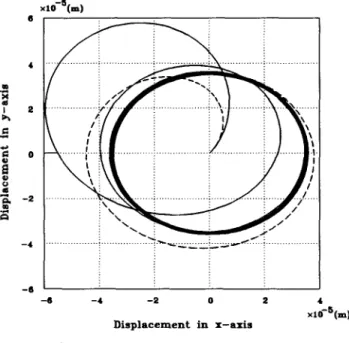
Control of a Rigid Rotor 4 -4 -6 -4 -2 0 2 4 .10-2(Bl) Displacement in x-axis

(a) Transient responses for & =l(solid

line) and &=lO’(dashed line)

-4 -2 -2 -I 0 1 2 3

Displacement in r-axis

(b) Transient response for 5 =lO’

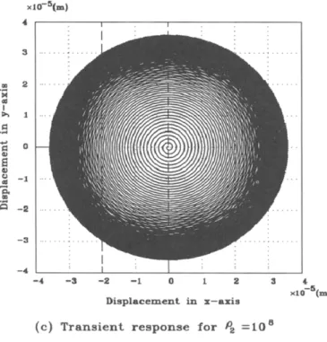
FIG. 7. Transient responses of the translational subsystem for the case of R = 1000 rad/sec and p, = 1.

Vol. 329, No. 6, pp. 1153~1178, 1992

Yi-Hua Fan et al. 4 3 .I 2 1 :: 1 a -_ ti 0 B 3 -1 5 a -2 -3 -4 1168 -4 -3 -2 -1 0 1 2 3 Displacement in x-axis (c) Transient response for p2 =lO’

x10-5(m) 4 3 .z 2 1 Al 1 E .” 2 0 B 0 -1 z s -2 -3 --I -4 -3 -2 -1 0 1 2 3 4 Displacement in x-axis x10-3(m)

(d) Transient response for p2 =lO”

FIG. 7. Continued.

Journal of the Franklm ,nst,tute Pergamon Press Ltd

Control of a Rigid Rotor

(a) Root loci for P, from 1 to l.Oe15 and P2 = 1

(b) Root loci for 4 from 1 to l.Oe15 and PI = 1

FIG. 8. Root loci of the translational subsystem

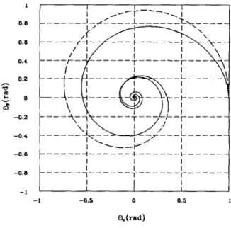
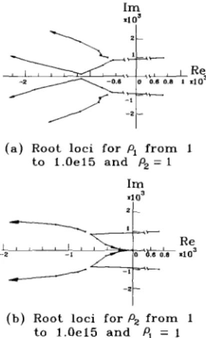
shows the case where p, changes from 1 to lOI while p2 = 1 ; Fig. 10 shows the case where p, = 1 and p2 changes from 1 to 10”. It is observed that the simulation results of this rotational subsystem are similar to those of the translational sub- system. Figure 11 shows the root loci of the subsystem of the rotational motions. The larger the weighting coefficient p ,, the more the damping ratio and the magnitude of stiffness. However, when the weighting coefficient pz increases, the magnitude of stiffness decreases.

4.2. The responses of the approximate rotational subsystem

Figure 12 gives the responses of the subsystem of the rotational motion which are respectively controlled by the optimal controller K, (as shown by a solid line) and the approximate optimal controller Ku (as shown by a dashed line), where X,(O) = [1 0 0 O]T and the weighting matrix is selected as Q = diag (l.Oef3, 1). We observed that the system controlled by an approximate optimal controller K, can still give a similar performance as that controlled by K,. As a matter of fact, since the longitude of shaft in this rotor system is larger than the radius of the shaft, the error resulting from the design procedure via approximation, in effect, is small. Due to this fact, the rotor system can be controlled by Ku if the longitude of shaft is larger than the radius.

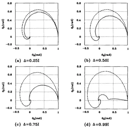
4.3. The efSect of the unsymmetrical moment qf inertia

If we neglected the asymmetrical moment of inertia, that is A = 0, then Eq. (19) can be rewritten as

Vol. 329. No 6, pp. 1153-l 178, 1992

Yi-Hua Fan et al. 1 0.0 0.6 0.4 0.2 0 -0.2 -0.4 -0.6 -0.8 -0.8 -0.4 -0.2 0 0.2 0.4 0.6 0.8 1 ‘Wad)

(a) Transient responses for 4 =l. 10’

(solid line),107 (dashed line), 10’

(dashdot line) and 10” (dotted line)

-0.2 0 0.2 0.6 0.6 I

(b) Transient response for P, =lO”

FIG. 9. Transient responses of the rotational subsystem for the case of R = 1000 rad/sec, initial condition X,(O) = [I 0 0 017 and p2 = 1.

Control of a Rigid Rotor 1 0.8 0.0 0.1 0.2

5

5

--

___J_,~rl_L__-lI_LL_-___

--

--

r .._

--i;_l+___&+p

---

--_--

_-_____j--LX+____-_;----__

(a) Transient responses for 4 = 1

(solid line) and 103(dashed line)

0.8 0.6 0.4 0.2 s t z 0 -0.2 -0.4 . . 1 -1 -0.5 0 0.5 1 4bd)

(b) Transient responses for 8 = 10’

(dashed line) and ld5(solid line)

FIG. 10. Transient responses of the rotational subsystem for the case of R = 1000 rad/sec, initial condition X,(O) = [l 0 0 01’ and p, = 1.

Vol 329, No. 6, pp. 1153-l 178, 1992

Yi-Hua Fan et al

(a) Root loci for PI from 1 to l.Oe15 and Pz = 1

Im .103

(b) Root loci for P2 from 1 to l.Oe15 and PI = 1 FIG. I 1. Root loci of the rotational subsystem

%(rad)

FIG. 12. Transient responses of the rotational subsystem controlled by the controller

K,, (dashed line) and K, (solid line) for the case of Q = 1000 radjsec, initial condition

X,(O) = [I 0 0 017 and p, = IO’, pz = I.

1172

Journal of the Franklin Institute Pcrgamon Press Ltd

Control of a Rigid Rotor -0.2 I 0.6 0.6 = 0.4 .z a 0.2 0 -0.2 -0.5 0 0.5 1 -0.5 0 0.5 1 6&d) 6&d)

(a) A=O.251 (b) A=O.501

-0.5 0 0.5 1 -0.5 0 0.5 1

6&d) 6&d)

(c) A=O.i’51 (d) A=O.991

FIG. 13. Transient responses of the rotational subsystem controlled by the controller K,, (dashed line) and K, (solid line) for the case of L2 = 1000 rad/sec, initial condition

X,(O) = [I 0 0 017 and p, = IO’, p2 = 1.

where X;.(t) = A&,(t)+B,U,.(t), 0 100 0 0 A0 = I b 0 Oa , Bo= kiL/21 0 0 0 01 0 0 0 -a b 0 I I 0 k, L/21 cl(21-1,)) b = <Q2(Zp-Z)+kdL* a=-~ Z Z 1. (31)

Substituting Eq. (31) into the Riccati equations, we can get an optima1 regulator K,. Figure 13 shows and compares the responses of the asymmetrical rotor system which are respectively controlled by the optimal regulator K, (as shown by a dashed Vol 329, No. 6, pp. IlS3~1178. 1992

Yi-Hua Fan et al.

line) and the optimal regulator K, (as shown by a solid line). Obviously, if the A is increasing, the performance of controller K,, becomes worse in quality than that of K,.

V. Conclusion

The equations of motion of the asymmetrical rigid rotor system have been derived via the theory of Hamilton’s principle. In order to construct a time- invariant control system, a coordinate transformation from the fixed coordinate system to the rotating coordinate system is used to simplify the equations of motion.

An optimal regulator which stabilizes the inherently unstable rotor-bearing system is presented by designing the controller in the rotating coordinate system. This makes the work of control design possible and easier. Moreover, if the longitude of the shaft is larger than its radius, an approximated model and its analytical-type controller are presented. From the simulation results, it is shown that the approximated controller also performs well. This leads to a good suggestion to simplify the control design for a long rotor system.

The vibration level and settling time are significantly affected by the chosen values of weighting coefficients p, and pz. To gain insight into the correlation between these coefficients and control performance, the root loci for various cases are compared; the results show that the weighting relevant to position term p, is more important than that relevant to velocity term p2. In addition, the influence due to the effect of the unsymmetrical moment of inertia has been accessed with various controller designs. The results further confirm the effectiveness of the proposed control scheme.

References

(1)

(2)

T. Yamamoto and H. Ota, “On unstable vibrations of a shaft carrying an unsym- metrical rotor”, J. uppl. Me&., Vol. 3 1, pp. 5 15-522, 1964.

T. Yamamoto and H. Ota, “On the forced vibrations of the shaft carrying an unsymmetrical rotor”, Bull. JSME, Vol. 9, pp. 58-66, 1966.

T. Yamamoto. H. Ota and K. Kono, “On the unstable vibrations of a shaft with unsymmetrical stiffness carrying an unsymmetrical rotor”, J. up@. Me&., Vol. 35,

pp. 313-321, 1968.

D. Ardayfio and D. A. Frohrib, “Instabilities of an asymmetric rotor with asym- metric shaft mounted on symmetric elastic supports”, J. Enyng Ind., Vol. 98, pp. 1161-l 165, 1976.

P. J. Brosens and S. H. Crandall. “Whirling of unsymmetrical rotor”, J. up@. Me&., Vol. 28, pp. 355-362, 1961.

G. Genta, “Whirling of unsymmetrical rotors : a finite element approach based on complex co-ordinates”, J. Sound Vib., Vol. 13 1, pp. 27-53, 1988.

Z. A. Parszewski, M. J. Krodkiewski and J. Rucinski, “Parametric instabilities of rotor-support systems with asymmetric stiffness and damping matrices”, J. Sound

Vib., Vol. 129, pp. 111-125, 1986.

F. Matsumura, H. Kobayshi and Y. Akiyama, “Fundamental equation for hori- Journal or the Franklin Inst~lute Pergamon Press Ltd

(9) (10) (II) (12) (13) (14) (IS) (16)

Control of a Rigid Rotor

zontal shaft magnetic bearing and its control system design”, Elec. Engng Japan,

Vol. 101, pp. 123-130, 1981.

T. Mizuno and 1’. Higuchi, “Design of the control system of totally active magnetic bearings-structures of the optimal regulator”, Proc. 1st lnt. Symp. Design and Synthesis, Tokyo, 1 l-13 July, pp. 534-539, 1984.

Z. Viderman and I. Porat, “An optimal control method for passage of a flexible rotor through resonances”, J. Dyn. Syst. Meas. Control, Vol. 109, pp. 216223,

1987.

J. R. Salm, “Active electromagnetic suspension of an elastic rotor : modeling, control, and experimental results”, J. Vib. Acoust. Stress Reliubil. Des., Vol. 110,

pp. 493-500, 1988.

A. B. Palazzolo, R. R. Lin, A. F. Kascak and R. M. Alexander, “Active control of transient rotordynamic vibration by optimal control methods”, J. Engng Gus

Turbines Power, Vol. 111, pp. 264-270, 1989.

K. Nonami, T. Yamanaka and M. Tominaga, “Vibration and control of a flexible rotor supported by magnetic bearings (control system analysis and experiments without gyroscopic effects)“, JSME ht. J., Series III, Vol. 33, pp. 475482, 1990. P. E. Allaire, D. W. Lewis and V. K. Jain, “Feedback control of a single mass rotor on rigid supports”, J. Franklin Inst., Vol. 312, pp. l-l 1, 1981.

P. E. Allaire, D. W. Lewis and V. K. Jain, “Active vibration control of a single mass rotor on flexible supports”, J. Franklin Inst., Vol. 315, pp. 21 l-222, 1983.

E. Anton and H. Ulbrich, “Active control of vibrations in the case of asymmetrical high-speed rotors by using magnetic bearings”, J. Vib. Acoust. Stress Reliabil. Des.,

Vol. 107, pp. 410415, 1985.

Appendix A Define

Jzn =

0

4i

[ -I, 0

1

(AlI

where I,, is the unit matrix of dimension n x n. J2,? has the following properties :

J,’ = J;, = - Jzn.

For the translational subsystem, the matrices A,, B,, Q and R satisfy

642)

J;‘ArJ4 = A,

J, ’ B, J, = B,

J:QJd = Q

J;RJ, = R.

Premultiplying Eq. (24) by JT and postmultiplying it by J4, it yields

J;P,A,J,+J;A:‘P,J,-J:P,B,Rm’B;P,J,+J:QJ, = 0.

Equation (A4) can be rewritten as

(A3)

(A4)

Vol. 329, No. 6, pp. 1153-l 178, 1992

Yi-Hua Fan et al.

(J:P,J4)(J4’A,J4)+(JJ’A,J4)7-(J:P,J4)-(J:P,J~)(J4’B,J2)

x (J;R-‘J2)(J, ‘B,J,)7(J,P,J,)+J:QJ, = 0. (A5) Substituting Eq. (A3) into Eq. (A5), we obtain

J:P,J,A,+A:J:P,J,-J;P,J,B,R ‘B;JdP,J4+J;QJ4 = 0. _W)

The positive definite solution of Eq. (24) also satisfies Eq. (A6). By the uniqueness of the solution, we have

P, = J:P,J, _(A7)

and

P, = P:. _WI

By using Eqs (A7) and (A8), we find that P, can be represented as

p,=

li:; ;;

Fj:

;Jq.

Substituting Eq. (A9) into Eq. (24), we obtain the following algebraic equations:

(A9)

Substituting Eqs (A12) and (Al3) into Eq. (AIO), we get

Equation (A14) has the unique solution satisfying pi,? > 0. and we can find the solution of p,, z as follows :

Control

qf a

IfD>O, thenp,,,= s+T-(a,i3), and if D < 0, thenp,,, = 2(- Y)“2~~~(0/3)-(a,/3),

where 0 = cos [Z/( - Y’) ‘:‘I, We have the other elements of P, as

Thus, P, = (pi(,) is the unique positive definite solution of Eq. (24).

Appendix B

As presented in Appendix A, for the rotational approximated subsystem an analytic solution P,, = (p,,,) satisfying the algebraic Riccati equation (30) can also be found. The matrix P, is represented as

p<,=

1;;

;; i; -;;I.

Substituting Eq. (Bl) into Eq. (30), we obtain the following algebraic equations

Substituting Eqs (B4) and (BS) into Eq. (B2), yields

Vol. 329, No. 6, pp. 11% 1178, 1992 Pnnted in Great Bntain

@I)

(B2)

(B3)

(B4)

Following the derivation in Appendix A, the unique positive solution of Eq. @6) satisfying P<,,~ z=- 0 can also be obtained. Then we have the other elements of P, as

Thus l’, = (F~,~~) is the unique positive definite solution of Eq. (30).

1178

journal of the Franklin Institute Pergamon presv Ltd