Extended Research on an Imperfect Process Production-inventory Model with Deteriorating Items under Two Dispatching Policies

兩種存貨派用策略下不完美製程損耗性商品

生產存貨模式之延伸研究

Extended Research on an Imperfect Process

Production-inventory Model with Deteriorating Items under

Two Dispatching Policies

宋振昌

1

June-Chun Sung

林正興

2

Chen-Sin Lin

宮大川

1

Dah-Chuan Gong

中原大學工業工程學系 中原大學工業工程學系

1

_{Department of Industrial Engineering, Chung-Yuan Christian University and}

2

_{Department of Industrial & Manufacturing Engineering & Technology, Bradley}

University

(Received June 13, 2007; Final Version March 17, 2008)

摘要：先進先出 (FIFO) 與後進先出 (LIFO) 為存貨管理最常預設的策略，其選用必需符合企 業實際生產情況，尤其當產品為易受製程偏移影響之損耗性商品。本研究首先針對不完美製程 損耗性商品提出FIFO 策略下之生產存貨模式，隨後應用指數函數之泰勒展開式推導出近似最佳 生產運轉時間之封閉解，並以數值範例說明模式精確性。再者，研究中將所獲得之模式與先前 提出之LIFO 策略生產存貨模式比較，並獲致損耗性商品於不完美製程生產時，LIFO 存貨派用 策略優於FIFO 策略之結論。最後，透過敏感度分析展現 FIFO 策略下各參數之影響。 關鍵詞: 存貨、損耗商品、不完美製程、先進先出、後進先出

Abstract: The First-In-First-Out (FIFO) and the Last-In-First-Out (LIFO) are the most general presumption policies of the inventory management. These presumptions are carefully considered in

The authors greatly appreciate the very valuable and helpful suggestions from Dr. Dennis E. Kroll. 本文之通訊作者為宋振昌，e-mail: [email protected]。

line with the actual practice of most business entities, especially when the merchandise or goods which have the deteriorating property affected by an imperfect production process. In this study, we firstly propose a production-inventory model for deteriorating items under an imperfect production process with FIFO inventory dispatching policy. Then, a closed-form solution of a near-optimal production uptime will be derived by utilizing Taylor series expansion of an exponential function. A numerical example is provided to argue the model’s fidelity. Also, a comparison with our previous research work—an LIFO policy production-inventory model is made. We conclude that when a deteriorating item is produced by an imperfect process, the LIFO inventory dispatch policy would be a better decision than the FIFO. Finally, sensitivity analysis is given to investigate the impacts that various parameters have in FIFO policy choice.

Keywords: Inventory, Deteriorating Item, Imperfect Process, FIFO, LIFO

1. Introduction

The economic production quantity (EPQ) model is an analytical model commonly adopted to cope with inventory management issues in a production-inventory system. This model is considered to be one of the most frequently adopted inventory control models which determine the optimal production lot size in cases of a single product produced on a single machine (Osteryoung et al., 1986). However, this model was developed under many idealistic but restricted assumptions. One limiting assumption of the EPQ model is that a production process is perfect during a production run. As a result, no defective item will be produced. However, in reality, manufacturing is affected by uncertainties in the environment of the production system, such as tool wear, vibration from operation of machines, unreliability of manual operations, defects of raw materials, and aging of equipment. Hence, a perfectly stable and reliable production process is rarely available in a real production environment (Nahmias, 2001). Another unrealistic assumption is that the items produced have indefinitely long lives. In general, aging and deterioration over time is the nature of all physical items. Many materials, such as highly volatile substances, radioactive materials, fresh food, blood, etc., their rates of deterioration are high. Loss from deterioration should not be ignored. Often the rate of deterioration is so low that it may be ignored in the determination of an optimal production lot size. However, in some cases, product deterioration may be aggravated if control of the production process is not accurate. When a production system may shift from an in-control state to an out-of-control

state during a production process and the items be produced may deteriorate significantly over time. For example, in the paper production process, if the alkaline reserve cannot be controlled at the proper concentration, the paper deterioration speed will increase and shorten the useful life of paper.

Many research results considering various inventory management models for deteriorating items have been given in the literature over the past several decades. Those who are interested can refer to those papers by Raafat (1991), Goyal and Giri (2001), and Lin et al. (2006). Lin et al. (2006) provided a brief literature review of production- inventory models considering the deterioration items; we omit another survey and only provide a review for papers that are directly related to our model. Ghare and Scharder (1963) developed the first Economic Order Quantity (EOQ) model for a single item under a constant rate of deterioration. Misra (1975) considered an EPQ model for deteriorating items with a varying rate of deterioration as well as a constant rate of deterioration. Mak (1982) studied a case with backordering for unfilled orders. Nevertheless, please note that the impact of an imperfect production process was not discussed in all of the aforementioned papers.

Over the past 20 years, studies on the impact of an imperfect process on the production cycle time or the production lot quantity have contributed considerable results. The studies conducted by Rosenblatt and Lee (1986) and Porteus (1986), are the first studies of the effects of an imperfect production process in determining the optimal production cycle time of an EPQ model. In their models, the production process may shift randomly from an in-control state into an out-of-control state during a production run. Once the process has shifted, a fixed portion of items produced becomes defective. All defective items are reworked or repaired with a cost. Several other research efforts also considered various inventory models that dealt with an imperfect production process (Lin, 1999; Giri et al., 2003; Chung and Hou; 2003). However, in the aforementioned research results, only Lin and Gong’s (2007) studied the deterioration of items and imperfect production process simultaneously. In their model, the inventory dispatching policy is LIFO. But in practice, a FIFO policy is the most general policy for inventory management. Hence, motivated by this, we extend Lin and Gong’s (2007) model and investigate in this paper an EPQ model for deteriorating items subject to an imperfect production process with a FIFO inventory dispatching policy. Under a FIFO policy, the units produced during out-of-control state will be stored first and then begin to be consumed after the units produced during the in-control state are depleted. The time epoch at which the process shifts into an out-of-control state is assumed to be a random variable which is exponentially distributed. A setup activity takes place before each production begins, and it restores the manufacturing process to its initial working condition.

In the next section, assumptions and notations for the model development are presented. The model itself will be addressed in Section 3 and a closed form of the optimal solution is also derived. Section 4 illustrates a numerical example to argue the model’s fidelity. Two figures have a hold on the convex property of the expected total cost function. In this research, we extend Lin and Gong’s (2007) work and apply a distinct policy to dispatch inventory. Therefore, the impact comparisons on the expected total cost between FIFO and LIFO policies will be discussed too. In Section 5, sensitivity analyses on the minimumexpected total cost Z(τ*_{) are supplied. Couple useful phenomena} are conducted. Finally, some concluding remarks will be given in the last section.

2. Assumptions and Notations

The mathematical model in this paper is developed on the basis of the following assumptions: (1) The demand rate of each product is known and finite.

(2) Lead time is zero and shortages are not allowed. (3) The production rate is finite.

(4) The system is in steady state, i.e., the production rate is greater than the demand rate. (5) Once an item (product) is produced, it is immediately available to meet the demand. (6) An item starts deteriorating at the moment when it is received into inventory. (7) The time-to-deterioration of an item follows an exponential distribution. (8) Deteriorated items are neither replaced nor repaired.

(9) Inventory holding cost is charged only to the amount of un-deteriorated stock.

(10) The cost of a deteriorated item is known and includes any disposal cost or salvage value. (11) Space and production lot size are not constrained.

(12) The production process may shift randomly from an in-control state into an out-of-control state during a production run. The time-to-shift is an exponentially distributed random variable. (13) The inventory system follows a FIFO policy. This implies that items produced during the

in-control state are consumed first and items produced during the out-of-control state are consumed later.

The notations employed in the paper are given as follows:

p production rate (items/unit time).

d demand rate (items/unit time).

Ii(t) inventory level function of good items at time t, produced during the out-of-control state, i = 2, 4, 5.

c cost of a deteriorated item ($/item). h inventory carrying cost ($/item/unit time). A setup cost of initiating a new production cycle.

α deterioration rate when the system is in the in-control state.

β deterioration rate when the system is in the out-of-control state, α < β.

X time-to-shift of the process from an in-control state to an out-of-control state.

λ parameter of an exponential distribution of the time-to-shift random variable. τ production uptime.

T1 the duration from the time point X to the end of production up-time τ, where T1= τ – x.

T2 the duration from the end of production up-time to the time point of inventories, which with α deterioration rate, be depleted.

T3 the duration from the time point of inventories, which with α deterioration rate, be depleted to the time point of inventories, which with β deterioration rate, be depleted.

T production cycle time including uptime and downtime.

Z(τ*_{) the minimum expected total cost when the optimal production uptime is}

_τ

*_.

3. The model

3.1 Model description

This paper deals with an EPQ model that considers the effect of a single facility imperfect production process on the optimal production uptime determination for deteriorating items under a FIFO policy. Under this operating policy, a production run is to be executed for a predetermined period of time (i.e., the production uptime). The items produced and consumed will follow a FIFO policy. Since the inventory is built up gradually during the production uptime, a new production run can only be started when all on-hand inventory items are depleted. A setup is required before each production run, and restores the production process to its initial working condition.

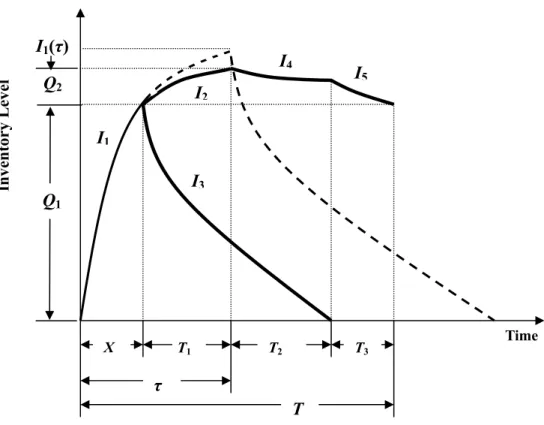
Although the time-to-shift is a random variable, we consider the time epoch from the beginning of each production run as a renewal epoch. A sample path representing the behaviour of the inventory system is depicted as in Figure 1. The path denoted by a dashed line illustrates a production cycle if no shift occurs. At time zero, the inventory level is zero and a production starts for a period of τ units

of time where the process is in the in-control state. In this time period, the inventory is gradually built up at a rate of p –d (where p>d). This rate is counteracted by a constant deterioration rate α. The inventory level increases up to its maximum level of I1(τ). After the maximum inventory is reached, production is terminated. From this point on, the on-hand inventory will be used to meet the demand and to counteract the losses due to the deterioration.

On the other hand, when a shift occurs at a random time point X before a production uptime τ is reached, i.e. a shift occurs at time x and x < τ, then items produced after this time point will have a higher deterioration rate. A sample path in this case is shown by the solid curve as in Figure 1. After the time point X, items with a higher deterioration rate β will be produced and the inventory will be built up with a rate p – d for another time period T1, where T1= τ – x. At the end of this period, the production run is terminated. The inventory been built-up should be enough to cover the losses due to deterioration for the remainder of the production cycle. In the time period T2, inventories built in the in-control state are continuously depleted till the end. The remaining inventory items contributed in the out-of-control state are then depleted in T3. Another production run will not begin until the

I

1

(τ)

I nventory Level

I

5

I

4

Q

2

I

3 Time

I

2

I

1 X T1 T2 T3

τ

T

Figure 1 Inventory level for a production cycle FIFO model

entire on-hand inventory being depleted. Note that in this case, the inventory level of items with a deterioration rate of β will be raised only up to Q2. In accordance with the FIFO policy, the on hand inventory with a lower deterioration rate of α will be depleted during the time period ofT1+T2. In other words, the inventory with β deterioration rate which is built-up after the process shift will be kept on hand during the time period of T2, and then be depleted to meet the demand during T3 period. The cycle time of the entire production cycle is T = τ +T2+T3.

Figure 1 shows that by conditioning on X = x, there are two cases to be considered depending on whether x ≥ τ or not. In the case where x ≥ τ, the model is similar to the one studied in Misra (1975). While for the case where x < τ, at the time point x, the inventory level of items produced in the in-control state reaches its maximum level, Q1. From this point onwards to the end of the production uptime, the system is in the out-of-control state. At the end of period T1, the amount of items in stock should be sufficient to cover the demand during the periods T2+T3. The cycle completes at the end of period T3. Let dIi(t) represent the change in the inventory level of each time period, during a small interval of time dt, which may be a function of the deterioration rate – α or β, the demand rate - d, and /or production rate - p. Therefore, the inventory level of the system at a time point t over the time interval (0, T) can be defined according to the different conditions by the following differential equations.

(1) Before the time point X, items with a lower deterioration rate of α will be produced and the inventory level will be built up to Q1 with a rate p - d. Therefore, the inventory level of the system at a time point t over the time interval (0, x) can be defined by the differential equation (1).

( )

_{( )}

1 1 d , for 0 d I t I t p d t X t +α = − ≤ ≤ . (1)

(2) After the time point X, items with a higher deterioration rate β will be produced and stocked. Therefore, the inventory level will be built up with a rate p for another time period T1 and can be defined by the differential equation (2).

( )

_{( )}

2 2 1 d , 0 d I t I t p for t T t +

β

= ≤ ≤ (2)

(3) During the time interval T1 + T2, the inventory level of the items with a lower deterioration rate α which was produced during the time interval (0, x) is continually consumed by demand. So, we can define I3(t) to be the inventory level function of the system and represent it by the differential

equation (3).

( )

_{( )}

3 3 1 2 d , 0 d I t I t d for t T T t +α = − ≤ ≤ + . (3)

(4) In the time period T2, the remaining inventory items with a deterioration rate β, which produced in the out-of-control state, are still in stock and deteriorating. So, we could define I4(t) function to represent the inventory level of the system.

( )

_{( )}

4 4 2 d 0, 0 d I t I t for t T t +β = ≤ ≤ . (4)

(5) After T2, the inventories which produced during the time interval (0, x) are all depleted. Therefore, the inventories with a deterioration rate of β are started to be used to support the demands and the losses due to the deterioration in T3.

( )

_{( )}

5 5 3 d - , 0 d I t I t d for t T t +β = ≤ ≤ . (5)

The boundary conditions for each differential equation are I₁

( )

0 =0 , I x₁

( )

=I₃

( )

0 = , Q₁

( )

( )

2 1 4

0

2

I T

=

I

=

Q

, I T₄

( )

₂ =I₅

( )

0 , and I T₅

( )

₃ =0.

The solutions for the above differential equations can be obtained as follows:

( )

(

-

)

1 1- , for 0 t p d I t eα t X

α

− = ≤ ≤ . (6)

( )

(

-

)

2 1- , for 0 1 t p I t eβ t T

β

= ≤ ≤ . (7)

( )

-3 1 , for 0 1 2 t d d I t Q eα t T T

α

α

⎛ ⎞ = − +_⎜ + _⎟ ≤ ≤ + ⎝ ⎠ . (8)

( )

- 4

,

2

for

0

2 t

I t

=

Q e

β

≤ ≤

t T

. (9)

( )

(

(3 )

)

5 1 , for 0 3 T t d I t eβ t T

β

− = − ≤ ≤ . (10)

(

)

1 1 x p d Q eα α − − = − . (11)

This implies that

( )

- αt - ( ) 3 1 2 p-d e - e ,for 0 α x t d p I t α t T T α α + = − + ≤ ≤ + . (12)

Next, using the initial condition I2(T1) = I4(0), we obtain

(

- 1

)

2 1 T p Q eβ β = − . (13)

This implies that

( )

(

1

)

4 1 T t p I t e β e β

β

− − = − . (14)

The objective of the model is to determine an optimal production uptime τ* _{that minimizes the} expected (long-run) total cost per unit time. As stated before, we consider the time epoch where each production run begins as a renewal epoch. Therefore, based on the renewal reward theorem (Ross, 2002), the expected total cost per unit time can be obtained by dividing the expected total cost per renewal cycle to the expected duration of a renewal cycle:

( )

E[

_{( )}

( )

]

_{( )}

( )

E[ ] G g Z T h

τ

τ

τ

τ

τ

= = . (15)

where E[G(τ)] and E[T(τ)] denote the expected total cost and the expected duration of a renewal cycle. Both are the functions of the production uptime τ.

3.2 An approximate solution

In this section, a closed-form solution as a near-optimal approximation to the production uptime is developed. Using the condition

I T

_{3 1}

(

+

T

₂

) 0

=

in equation (12), we obtain

(

1 2

)

(

1 2

)

- T T _- - - x T T ₀ d p p d eα e α α α α + + + − + = . (16)

If we use the relation T₁= −

τ

x and Taylor series approximation for exponential functions in equation (16) and assume αT << 1, we obtain an expression for T2 in terms of τ and x as follows: (see Appendix A)

2 2 1 2 px p x p T d d d α τ ⎛ ⎞ ≈ − + + _⎜ − _⎟ ⎝ ⎠

(

)

2 1 ₂ 2 p p d p d T x x d d

α

− − ⎛ ⎞ = − +_{⎜ ⎟} − ⎝ ⎠ . (17)

From Figure 1, it can be concluded that I4(T2) = I5(0). This implies that

(

)

2 1 -3 1 ln 1 p T 1- T T e e d β β

β

− ⎛ ⎞ = _⎜ + _⎟ ⎝ ⎠. (18)

By referring to the relation of T1 and T2, neglecting β2 and the higher order of β, applying the Taylor series approximation again to simplify the exponential item in equation (18), we can describe the T3as follows: (see Appendix B)

(

)

2 3 - 1 - - 1 -2 p p p T x x x d d d

β

α

τ

⎡ ⎛ ⎞ ⎛

τ

⎞⎤ ≈ _{⎢ ⎜ ⎟ ⎜} + _⎟⎥ ⎝ ⎠ ⎝ ⎠ ⎣ ⎦ . (19)

This allows us to express the production cycle time, denoted by T(1) _{for the case of x < τ:} 2 (1) _{1 ( ) 1 1} 2 2 2 px p x p p p p T x x x d d d d d d

α

⎛ ⎞

_τ

⎡

β

⎛ ⎞⎛

_τ

α

⎞⎤ = + _⎜ − _⎟+ − _⎢ − _⎜ − _⎟⎜ + − _⎟⎥ ⎝ ⎠ ⎣ ⎝ ⎠⎝ ⎠⎦. (20)

And, the production cycle time, denoted by T(2) _{, for the case of x > τ, is formulated as follows:}

2 (2) 1-2 p p p T d d d

τ

ατ

⎛ ⎞ = + _{⎜ ⎟} ⎝ ⎠. (21)

Since the time-to-shift is an exponentially distributed random variable with a mean of 1/λ, the expected cycle time of a production cycle can obtained as follows:

(1) (2) 0 E[ ( )] xd xd T T e x T e x τ λ λ τ

τ

₌

λ

− ₊∞

λ

−

∫

∫

. (22)

After carrying out the calculation and neglecting the terms with higher power of terms including α2_{, β}2_,

αβ, and λτ, we have

(

)

2

(

)(

)

3 2 / 1 E[ ( )] 2 3 2 p p d p d p T p d d d d α β α τ λ τ = − − τ −λ ⎡_⎢ − − + ⎤_⎥τ ⎣ ⎦ . (23)

Let IH denote the amount of inventory hold during a cycle and DI denote the number of deteriorating items. Hence, for the case of x < τ, we obtain

( )

1

( )

1 2

( )

2

( )

3

( )

(1) 1 2 3 4 5 0 0 0 0 0 d d d d d T T T T T x IH I t t I t t I t t I t t I t t + =

_∫

+

_∫

+

_∫

+

_∫

+

_∫

(

)

2

(

)(

)

(

2 2

)

2 2 2 2 2 p x p d x x p p d d d

τ

β τ

α

τ

− − ⎡ − + ⎤ − _{⎣ ⎦} = − . (24)

Because the inventory holding cost is assumed to be charged only to the amount of un-decayed stock, so the second item of equation (24) can be ignored. We then have the IH(1) _{presented as follows:}

(

)

(1) 2 2 p p d IH d

τ

− = . (25)

Furthermore, DI can be obtained by finding the difference between the amount produced and the demand. This means

(1)

(

)

(

)

2 3 = - -DI px d τ+T + p τ −x dT

(

2 2

)

2 1 2 p p x x d

β τ

α

⎛ _{⎞ ⎡ ⎤} = _⎜ − _{⎟ ⎣} − + _⎦ ⎝ ⎠ . (26)

Hence, for the case of x > τ, we have

(

)

(2) 2

2

p p d

IH

d

τ

−

=

. (27) 2 (2) ₁ 2 p p DI d

ατ

⎛ ⎞ = _⎜ − _⎟ ⎝ ⎠. (28)

The total cost function including setup, inventory holding, and deterioration costs can be written as follows:

( )

G

τ

= + ×A h IH c DI+ × . (29)

For the case x < τ, by substituting equations (25) and (26) into equation (29), we obtain

( )

(1) (1) (1)

(

)

2 ₁

₍

₍

2 2

₎

2

₎

2 2 p p d p p A h c x x d

τ

d

β τ

α

⎡ − ⎤ ⎡ ⎛ ⎞ ⎤ = + _{⎢ ⎥}+ _{⎢ ⎜} − _⎟ − + _⎥ ⎝ ⎠ ⎣ ⎦ ⎣ ⎦ . (30)

For the case of x > τ, by substituting equations (27) and (28) into equation (29) we obtain the total cost per cycle as follows:

( )

(2) (2) (2) G

τ

= + ×A h IH + ×c DI

(

)

2 2 ₁ 2 2 p p d p p A h c d d

ατ

τ

⎡ − ⎤ ⎡ ⎛ ⎞⎤ = + _{⎢ ⎥}+ _{⎢ ⎜} − _⎟⎥ ⎝ ⎠ ⎣ ⎦ ⎣ ⎦ . (31)

Hence, the expected total cost per cycle can be expressed as

(1) (2) 0 E[ ( ) ]_G τ_{G e} λxd_{x G e} λxd_x τ

τ

₌

λ

− ₊∞

λ

−

∫

∫

. (32)

After some algebra and neglecting the terms with a higher power λτ, we obtain

2 3 ( )( ) ( )( ) E[ ( ) ] 2 3 p p d h c cp p d G A d d

α

λ

β α

τ

= + − +

τ

+ − −

τ

. (33)

Using equation (15), the expected total cost per unit time can be expressed as follows:

( )

_{( )}

( )

(

)(

)

(

)(

)

(

)

(

)(

)

2 3 2 3 2 E[ ] _{2 3} E[ ] / 1 2 3 2 p p d h c cp p d A G _{d d} Z T p p p d p d p d d d d α λ β α τ τ τ τ τ τ α _{τ λ} β α λ _τ − + − − + + = = ⎡ ⎤ − − − − − _⎢ + _⎥ ⎣ ⎦ . (34)

For further discussion, let

1 = ,A ω 2 ( )( ) = , 2 p p d h c d

α

ω

− + 3 ( )( ) = , 3 cp p d d

λ

β α

ω

− − 4 = , p d

ω

5 2 ( ) = , 2 p p d d

α

ω

− 6 ( )( / 1) = 3 2 p d p d d

β α

λ

ω

λ

⎡_⎢ − − + ⎤_⎥ ⎣ ⎦.

Hence, we could have a simple configuration of function Z(τ).

2 3 1 2 3 2 3 4 5 6 ( ) Z

τ

ω ω τ

ω τ

ω τ ω τ

ω τ

+ + = − − . (35)

In order to determine a near optimal production uptime that minimizes Z(τ), we quote the property due to Bazaraa et al. (2006).

Property 1.

Let two function g: S → E1 and h: S → E1, where S is a nonempty convex set in En. Consider the function f: S → E1 defined by f(x) = g(x)/h(x). Then f is a pseudoconvex if the following two

conditions hold true: (a) g is convex on S, and g(x)

≥

0 for each x

∈

S, (b) h is concave on S, and h(x)

>

0 for each x

∈

S, and (c) both g and h are differentiable.

Proof. Obvious. Property 2.

The function given in Z(τ) is pseudoconvex for τ > 0. Proof.

From Property 1, we can prove that Z( )

τ

is a pseudoconvex function by showing the convexity of E[G(τ)] and the concaveness of E[T(τ)]. This can be shown by finding the second derivative of each function as follows:

( )

(

)(

)

(

)(

)

2 2 d E[ ] 2 d G p p d h c cp p d d d

τ

α

λ

β α

τ

τ

− + − − = + . (36)

( )

(

)

(

)(

)

2 2 2 d E[ ] 2 / 1 3 d T p p d p d p d d τ α β α λ λ τ τ ⎡ ⎤ − − − + = − − _{⎢ ⎥} ⎣ ⎦ . (37)

Since p > d, α < β, so _d2_{E[ ( )]G}

_τ

_d

_τ

2 _{>0 and d}2_{E[ ( )]T τ dτ <}2 _{0 for τ > 0, and both functions} are continuous. Referring to Property 1, we can conclude that

Z

( )

τ

is pseudoconvex.

Let dZ( ) /

τ

d

τ

=0. Then, the near optimal solution of τ that minimizes Z(τ) can be found by solving the equation

(

)

4 3

(

)

2

2 6 3 5

2

3 4 2 4

3

1 6

2

1 5 1 4

0

ω ω ω ω τ

−

+

ω ω τ

+

ω ω

+

ω ω τ

+

ω ω τ ω ω

−

=

. (38)

The positive root of the above equation can be solved by using numerical approaches such as the bisection methods and Newton’s methods. One can also apply the Excel Goal Seek function to obtain a solution. However, it is still complicated to solve the equation (38) directly. To simplify the problem, we ignore the fourth degree term of

τ

and transfer the equation (38) into a cubic equation as follows.

(

)

3 2

3 4 2 4 1 6 1 5 1 4

2

ω ω τ

+

ω ω

+

3

ω ω τ

+

2

ω ω τ ω ω

−

=

0

(39)

After some algebraic solving procedures, a closed-form of near optimal solution of τ can be obtained as in the following:

(

2

)

2 4 3 * 3 4 4 4 2 3 6 3 3 u u u _u v u vu u τ = − − − . (40) where 1 = 1 4 u

ω ω

,

u

₂

= 2

ω ω

_{1 5},

u

₃

= 3

ω ω ω ω

_{1 6}

+

_{2 4}, u₄ = 2

ω ω

_{3 4}, and

(

)

1 3 2 3 3 2 2 2 2 3 2 3 4 1 4 3 4 2 4 2 3 1 2 3 4 1 4 1 3 = 36 +108 -8 +12 3 4 - +18 +27 -4 v u u u u u u u u u u u u u u u u u u u .

Note that when

β α

= =

0,

the production uptime in equation (39) becomes the optimal production uptime for the classical EPQ model.

1 2 * 0, 0 2 lim ( ) Ad hp p d α→ β→τ ⎛ ⎞ = ⎜ ₋ ⎟ ⎝ ⎠ .

4. Illustrative example

The following parameters are used to illustrate the application of the model. Let production capacity be 7500 units per year and the demand rate be 2500 units per year. Other related factors are as follows: the production setup cost is $45 per order, the inventory holding cost is $0.5 per unit per year, and the deterioration cost is $5 per unit. Both the time-to-shift of productions system and the time-to-deterioration of an item are assumed to be an exponential distribution. The deterioration rates

at the in-control state and out-of-control state are 0.02 and 0.2, respectively. The mean time of the time-to-shift is assumed 10. Solving equation (40) gives the optimal production uptime (

τ

*) a value of 0.0527. Furthermore, substituting the optimal production uptime into equation (34) yields the minimum expected total cost per unit time, Z(

τ

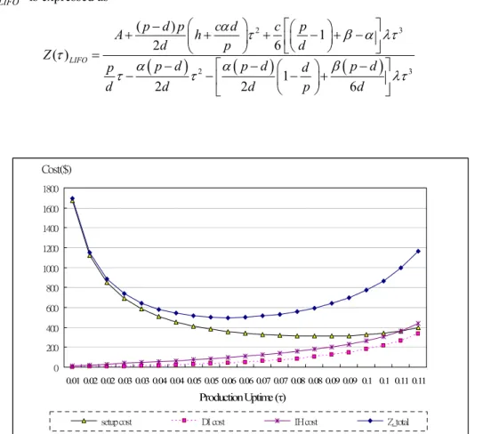
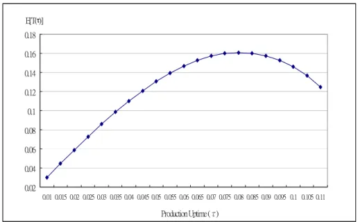
*), a value of $473.11.

Figure 2 shows the inventory of function Z(τ) and the changes of each cost component to the production uptime. The inventory holding cost and the deterioration cost increase along with the increasing of the production uptime. Figure 3 demonstrates the argument that E[T(τ)] is a concave function.

This research is extended from Lin and Gong’s (2007) work, in which an LIFO policy is applied. We are interested in comprising the impacts on the expected total cost when two distinct policies (ie., FIFO and LIFO) are concerned. The expected total cost function of LIFO policy denoted by

( )

_LIFO

Z

τ

is expressed as

(

)

(

)

(

)

2 3 2 3 ( ) 1 2 6 ( ) 1 2 2 6 LIFO p d p c d c p A h d p d Z p d p d p d p d d d d p d α _{τ β α λτ} τ α α β τ τ λτ ⎛ ⎞ ⎡ ⎤ − ⎛ ⎞ + _⎜ + _⎟ + _⎢⎜ − + −_{⎟ ⎥} ⎝ ⎠ ⎣ ⎦ ⎝ ⎠ = ⎡ ⎤ − − ⎛ ⎞ − − −_{⎢ ⎜} − _⎟+ _⎥ ⎝ ⎠ ⎣ ⎦ (41) 0 200 400 600 800 1000 1200 1400 1600 1800 0.01 0.02 0.02 0.03 0.03 0.04 0.04 0.05 0.05 0.06 0.06 0.07 0.07 0.08 0.08 0.09 0.09 0.1 0.1 0.11 0.11 Production Uptime (τ) Cost($)

setup cost DI cost IH cost Z_total

E[T(τ)] 0.02 0.04 0.06 0.08 0.1 0.12 0.14 0.16 0.18 0.01 0.015 0.02 0.025 0.03 0.035 0.04 0.045 0.05 0.055 0.06 0.065 0.07 0.075 0.08 0.085 0.09 0.095 0.1 0.105 0.11 Production Uptime (τ)

Figure 3 System production cycle time as a function of production uptime.

Let β be fixed to 0.2 and φ be the ratio of deterioration rate α to the deterioration rate β. Given different values of φ, Table 1 shows the results on τ*_{and Z}* _{with respect to FIFO and LIFO policies.} We observe that no matter what values of φ are, the LIFO policy always provides a lower expected total cost. We should not make a conclusion just based on couple instances. However, those comparisons in Table 1 indeed reveal a solid suggestion. This is also a contribution of this paper.

Table 1 Comparison between FIFO and LIFO ploicy

ϕ

FIFO LIFO * FIFO

τ

* FIFO

Z

* LIFO

τ

* LIFO

Z

0 0.05306 462.8358 0.10911 274.5965 0.2 0.05238 483.3502 0.10225 292.9125 0.4 0.05168 503.653 0.09653 310.1932 0.6 0.05097 523.7382 0.09167 326.5997 0.8 0.05024 543.6006 0.08746 342.2554

5. Sensitivity analysis

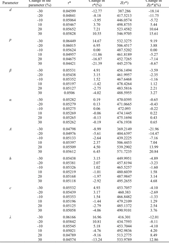
In this section, we study the effects in the parameters set {d, p, α, β, A, h, c, λ} on the optimal values of τ* _{and Z(τ}*_{) derived by the proposed FIFO model. The sensitivity analysis is performed by} changing each parameter set by -30%, -20%, -10%, 10%, 20% and 30% with all other parameters remaining unchanged. On the basis of the result shown in Table 2, the following observations can be made.

(1) There is a decrease in the τ* _{values when p, β, α, h, c or λ increase.} (2) There is an increase in the τ* _{values when d or A increase.}

(3) The expected total cost Z(

τ

*) increases with an increase in d, β, α, A, h, c or λ, but it decreases with an increase in p since the production rate increased.

(4) The expected total cost Z(

τ

*) is very highly sensitive with respect to A, highly sensitive to d and λ, but almost insensitive to a change in α.

From the above analysis, it is seen that A is a critical parameter in the sense that any change in A results in significant change in the expected total cost Z(

τ

*).

6. Conclusions

In this paper, we have developed an EPQ model for deteriorating items to be produced on an imperfect process that is subject to a random shift from in-control state to out-of control state and a FIFO inventory dispatching policy is considered. This scenario had not been considered in the Misra’s model (1975). The items produced in the out-of-control state are subject to a higher than normal deterioration rate. The time for the process shift to the out-of-control state and the time to deterioration are assumed to be exponentially. The objective is to determine a near optimal production uptime so as to minimize the expected total cost per unit time consisting of setup, inventory holding, and deterioration costs. Based on numerical examples illustrated in this paper, the following conclusions can be made:

(1) Applying FIFO policy, the expected total cost Z(

τ

*) is highly sensitive in respect to setup cost per order, A, and slightly sensitive in respect to a change in the deterioration rate after process shift, β. But, Z(

τ

*) is almost insensitive to a change in the deterioration rate before process shift, α. (2) When a deterioration item is produced in an imperfect process, the LIFO inventory dispatching

Table 2 Results of the sensitivity analysis on different parameters

Parameter _{parameter (%)} Change in the τ* Change in _τ*(%) Z(τ*) Change in _Z(τ*)(%)

d _-30 -20 -10 10 20 30 0.04599 0.04841 0.05064 0.05467 0.05652 0.05828 -12.77 -8.18 -3.95 3.70 7.21 10.55 387.286 417.5213 446.0574 498.8755 523.4582 546.9705 -18.14 -11.75 -5.72 5.44 10.64 15.61 p _-30 -20 -10 10 20 30 0.06449 0.06015 0.05624 0.04957 0.04675 0.04421 14.67 6.95 0.00 -11.86 -16.87 -21.39 532.3275 506.4517 487.5202 461.8189 452.7265 445.2576 9.19 3.88 0.00 -5.27 -7.14 -8.67 β -30 -20 -10 10 20 30 0.05531 0.05438 0.05352 0.05197 0.05127 0.0506 4.91 3.15 1.52 -1.42 -2.75 -4.02 456.1494 461.9957 467.6468 478.4264 483.5816 488.5955 -3.59 -2.35 -1.16 1.12 2.21 3.27 α -30 -20 -10 10 20 30 0.05282 0.05279 0.05275 0.05269 0.05265 0.05262 0.19 0.13 0.06 -0.06 -0.13 -0.19 470.0395 471.0665 472.093 474.1445 475.1694 476.1938 -0.65 -0.43 -0.22 0.22 0.43 0.65 A -30 -20 -10 10 20 30 0.04798 0.04976 0.05133 0.05397 0.05509 0.05612 -8.99 -5.61 -2.64 2.37 4.50 6.45 369.2149 404.6397 439.2225 506.4453 539.2902 571.7235 -21.96 -14.47 -7.16 7.04 13.99 20.84 h -30 -20 -10 10 20 30 0.05438 0.05381 0.05326 0.05219 0.05168 0.05118 3.15 2.07 1.02 -1.01 -1.97 -2.92 449.9951 457.8194 465.5257 480.6039 487.9847 495.2655 -4.89 -3.23 -1.60 1.58 3.14 4.68 c -30 -20 -10 10 20 30 0.05532 0.05439 0.05353 0.05196 0.05125 0.05058 4.93 3.17 1.54 -1.44 -2.79 -4.06 453.7057 460.383 466.8482 479.2109 485.1372 490.9101 -4.10 -2.69 -1.33 1.29 2.54 3.76 λ -30 -20 -10 10 20 30 0.06166 0.05842 0.05545 0.05021 0.04789 0.04574 16.96 10.81 5.18 -4.76 -9.16 -13.24 416.301 434.7593 453.7044 492.9836 513.2775 533.9789 -12.01 -8.11 -4.10 4.20 8.49 12.86

The second conclusion does not exactly low down the value of the FIFO model. On the other hand, because of the firm procedure provided in the FIFO model development and significant distinctions shown in Table 1, we then are able to have that summary. These two conclusions demonstrate solid suggestions in practice and the contribution about the proposed model. Future research directions can be models with effects such as price-dependent demand and other distributions for deterioration.

Appendix A: The detail derivation process of T

2

.

Here,

T

₁

= −

τ

x

, hence, we can derive from equation (16) that

(

2

)

(

2

)

- T x _- - - T ₀ d p p d e α τ e α τ α α α + − + − + = . (A1)

By solving (A1), we can get

2 ln _xd pe p d T α ατ α ⎛ ⎞ + ⎜_⎜ ⎟_⎟ − + ⎝ ⎠ = − (A2) 1 ln 1 x p e d α τ α ⎛ ₋ ⎞ = − ⎜_⎜ ⎟_⎟ ⎝ ⎠ 1 （ ） ＋ ＋ .

Using the expansion of the natural logarithm function ln (1+y), ln(1+y) = y - y2_{/2 + y}3_{/3 - y}4_{/4 + …,} where -1<y≤1. Keeping the first two terms of the series, then

2 ln(1 ) 2 y y y + ≈ − . Consequently, the approximation value of T2 can be given as

2 ( ₂ 2 x x pe p pe p T d _d α α

τ

α

⎛ _{− −} ⎞ ≈ − ⎜_⎜ − ⎟_⎟ ⎝ ⎠ 2 1 ） ＋ . (A3)

Since αx << 1, then, by using the Taylor series approximation to the exponential items in (A3) and omitting the high order item of α which is larger than 2, we can derive

2 ( ) 1 2! x x eα ≈ +

α

x+

α

. (A4)

By inserting (A4) into (A3), we can obtain

2 2 2 p 1 ( ₂x) 1 1 ₂p (1 ( ₂x) 1) T x x d d

α

α

τ

α

α

α

⎛ ⎞⎛ ⎞ = − + ⎜_⎜ + + − ⎟⎜_⎟⎜ − + + − ⎟_⎟ ⎝ ⎠⎝ ⎠ 2 2 2 2 2 ( ) ( ) 2 ₂ 2 p x p x x x d _d

α

α

τ

α

α

α

_α

⎛ ⎞ ⎛ ⎞ = − + ⎜_⎜ + ⎟_⎟− ⎜_⎜ + ⎟_⎟ ⎝ ⎠ ⎝ ⎠ 2 4 4 2 2 3 3 2 1 2 ₂ 4 px x p x x x d _d α α τ α α α ⎛ ⎞ ⎛ ⎞ = − + _⎜ + _⎟− ⎜_⎜ + + ⎟_⎟ ⎝ ⎠ _{⎝ ⎠}.

Clearly, if we omit the high order terms of α which is larger than or equal to 2 and simplify the equation, we can get

2 2 2 1 _{2 2} 2 px x p x T d d α α τ ⎛ ⎞ = − + _⎜ + _⎟− ⎝ ⎠ 2 1 2 px p x p d d d

α

τ

⎛ ⎞ = − + + _⎜ − _⎟ ⎝ ⎠.

Appendix B: The detail derivation process of T

3

.

Since I4(T2) = I5(0), thus, we can derive from equations (9) and (10) that

(

) (

)

(

3 1 2

)

1 1 1 T T T d eβ p e β e β

β

− − − − − =0. (B1)

By solving (B1), we can get

2 1 3 1ln 1 (1 ) T T pe e T d β β

β

− − ⎛ ₋ ⎞ = ⎜_⎜ + ⎟_⎟ ⎝ ⎠ . (B2)

where -1<y≤1. Keeping the first two terms of the series, then 2

ln(1

)

2

y

y

y

+

≈ −

.

Consequently, the approximation value of T3 can be given as

2 1 2 1 2 3 1 (1 ) 1₂ (1 ) T T T T pe e pe e T d d β β β β

β

− − − − ⎛ _{⎛ ⎞} ⎞ − − ⎜ ⎟ ≈ _⎜ − ⎜_⎜ ⎟_{⎟ ⎟} ⎜ _{⎝ ⎠} ⎟ ⎝ ⎠ . (B3)

Since βT1<< 1 and βT2<< 1, then, by using the Taylor series approximation to the exponential terms in (B3) and omitting the high order terms of β which is larger than 2, we can get

1 2 1 1

(

)

1 (

)

2

T

T

e

−β

= + −

β

T

+

−

β

, and 2 2 2 2 ( ) 1 ( ) 2 T T e−β = + −

β

T + −

β

. (B4) Substituting (B4) into (B3), we find

(

)

(

)

(

)

(

)

2 2 2 1 _{2 2} 2 1 2 1 3 2 1 (1 )( ) 1 _{2 2} 1 (1 )( ) 2 2 2 T T p T T _{p T T} T T T d d β β β β _{β β} β β β − − − + − _{⎛ − − ⎞} ⎜ ⎟ = − − + − ⎜ ⎟ ⎝ ⎠ 2 2 2 2 2 3 2 2 1 1 2 2 1 1 2 1 1 2 2 2 2 4 T T T T T T T p T T T d β _β β β β ⎛ ⎞ = _⎜ − − + + − _⎟ ⎝ ⎠ 2 2 3 2 3 2 4 2 2 2 1 1 2 2 1 1 2 1 1 2 1 ( ) 2 2 2 2 4 T T T T T T T p T T T d β β β β β β ⎛ ⎞ − − − + + − ⎜ ⎟ ⎝ ⎠.

By omitting the high order terms of β which is larger than or equal to 2, we can have: 2 1 1 3

(

1 1 2

)(1

)

2

2

T

p T

p

T

T

TT

d

d

β

_β

β

=

−

−

−

2 2 2 3 2 2 1 1 1 1 2 1 1 2 ( ) 2 2 4 2 T p T p T p T T p T TT d d d d

β

_β

β

β

β

= − − − + + .

Still, we can omit the high order terms of β which is larger than or equal to 2 and simplify the equation, thus, the equation of T3 can be

2 2 1 1 3

(

1 1 2

)

2

2

T

p T

p

T

T

TT

d

d

β

_β

β

=

−

−

−

(

)

1 1 2 2

2

(

)

2

2

pT

d

p d T

dT

d

β

β

−

+

−

=

. (B5)

Substituting

T

₁

= −

τ

x

and (17) into (B5), after some simplifications, we thus obtain

(

)

2 3 - 1 - - 1 -2 p p p T x x x d d d β α τ ⎛ ⎛ ⎞ ⎛τ ⎞⎞ = _{⎜ ⎜ ⎟ ⎜} + _⎟⎟ ⎝ ⎠ ⎝ ⎠ ⎝ ⎠ .

References

Bazaraa, M. S., Sherali, H. D., and Shetty, C. M., Nonlinear Programming: Theory and Algorithms, 3rd ed., New York: John Wiley & Sons, 2006.

Chung, K.-J. and Hou, K.-L., “An Optimal Production Run Time with Imperfect Production Processes and Allowable Shortages,” Computers & Operations Research, Vol. 30, No. 4, 2003, pp. 483-490. Giri, B. C., Moon, I., and Yun, W. Y., “Scheduling Economic Lot Ssizes in Deteriorating Production

Systems,” Naval Research Logistics, Vol. 50, Iss. 6, 2003, pp. 650-661.

Ghare, P. M. and Schrader, G. F., “A Model for Exponential Decaying Inventory,” Journal of Industrial Engineering, Vol. 14, No. 5, 1963, pp. 238-243.

Goyal, S. K. and Giri, B. C., “Recent Trends in Modeling of Deteriorating Inventory,” European

Journal of Operational Research, Vol. 134, Iss.. 1, 2001, pp. 1-16.

Lin, C.-S., “Integrated Production-inventory Models with Imperfect Production Processes and A Limited Capacity for Raw Materials,” Mathematical and Computer Modeling, Vol. 29, Iss. 2, 1999, pp. 81-89.

Lin, G. C., Dennis, E. K., and Lin, C. J., “Determining a Common Production Cycle Time for an Economic Lot Scheduling Problem with Deteriorating Items,” European Journal of Operational

Research, Vol. 173, Iss. 2, 2006, pp. 669-682.

Lin, G. C. and Gong, D.-C., “On a Production-inventory Model for Deteriorating Items Subject to an Imperfect Process,” Journal of the Chinese Institute of Industrial Engineers, Vol. 24, No. 4, 2007, pp. 319-326.

Mak, K. L., “A Production Lot Size Inventory Model for Deteriorating Items,” Computers and

industrial engineering, Vol. 6, No. 4, 1982, pp. 309-317.

Misra, R. B., “Optimum Production Lot Size Model for a System with Deteriorating Inventory,”

Nahmias, S., Production and Operations Analysis, 4th ed., Boston: McGraw-Hill Irwin, 2001.

Osteryoung, J. S., Nosari, E., McCarty, D. E., and Reinhart, W. J., “Use of EOQ Model for Inventory Analysis,” Production and Inventory Management, Vol. 27, Iss. 3, 1986, pp. 39-45.

Porteus, E. L., “Optimum Lot Sizing, Process Quality Improvement and Setup Cost Reduction,”

Operations Research, Vol. 34, Iss. 1, 1986, pp.137-144.

Raafat, F., “Survey of Literature on Continuously Deteriorating Inventory Models,” Journal of

Operational Research Society, Vol. 42, Iss. 1, 1991, pp. 27–37.

Rosenblatt, M. J. and Lee, H. L., “Economic Production Cycles with Imperfect Production Process,”

IIE Transactions, Vol. 18, Iss. 1, 1986, pp. 48-55.