用於自動對焦數位相機之音圈馬達及其伺服控制IC之分析與設計

國 立 交 通 大

國 立 交 通 大

國 立 交 通 大

國 立 交 通 大 學

學

學

學

電 機 與 控 制 工 程 學 系

碩 士 論 文

用於自動對焦數位相機之音圈馬達及其伺服控

制IC之分析與設計

Design and Analysis of a Voice Coil Motor with the

Servo Control IC for Auto-Focusing Digital Cameras

研 究 生：許智達

指導教授：鄒應嶼 博士

用於自動對焦數位相機之音圈馬達及其伺服控

用於自動對焦數位相機之音圈馬達及其伺服控

用於自動對焦數位相機之音圈馬達及其伺服控

用於自動對焦數位相機之音圈馬達及其伺服控

制

制

制

制IC之分析與設計

之分析與設計

之分析與設計

之分析與設計

Design and Analysis of a Voice Coil Motor with the

Servo Control IC for Auto-Focusing Digital Cameras

研 究 生：許智達

Student: Jhih-Da Hsu

指導教授：鄒應嶼 博士 Advisor: Dr. Ying-Yu Tzou

國立交通大學

電機與控制工程學系

碩士論文

A Thesis

Submitted to Department of Electrical and Control Engineering College of Electrical Engineering and Computer Science

National Chiao Tung University in Partial Fulfillment of the Requirements

for the Degree of Master in

Electrical and Control Engineering July 2007

Hsinchu, Taiwan, Republic of China

用 於 自 動 對 焦 數 位 相 機 之 音 圈 馬 達 及 其 伺 服 控 制 IC之

分 析 與 設 計

研究生：許智達

指導教授：鄒應嶼 博士

國立交通大學電機與控制工程學研究所

摘

摘

摘

摘

要

要

要

要

本篇論文說明用於行動電話之數位相機自動對焦控制系統之音圈馬達設計與建 模，並針對此自動對焦模組提出控制器設計方法，使用 FPGA 實現全數位之定位控制 IC。在音圈馬達中，由於其機械結構及磁路架構，力常數及反抗電動勢常數呈現高度非 線性之特性。傳統透過幾何結構導出磁力線分佈以鑑別馬達之等效參數的建模方式過於 複雜且不切實際。針對此特殊用途之音圈馬達，基於其機械結構及材料，藉由 Ansoft 公司之電磁模擬軟體 Maxwell 2D，發展一套建立其數學模型之流程。本文所使用之音圈 馬達乃非傳統使用於手機相機自動對焦系統致動器之步進馬達或需要彈簧之音圈馬 達。為了達到在受限的體積之下，具有最大之力常數之音圈馬達設計，本篇論文提出一 套利用模擬軟體輔助設計之方法。最後模擬與實驗結果之比對將呈現模型之正確性及其 所滿足之效能。根據音圈馬達之建模與設計，其伺服驅動控制 IC 設計規劃中包含數位 伺服控制器、數位電流迴路及全橋式直流-直流轉換器。針對高效能、輕薄型手機相機 及錄像機之鏡頭自動對焦定位控制，此伺服控制 IC 提供全數位化之方法。此自動對焦 系統直線運動範圍全行程為 0.6 mm，在 30 ms 內定位，且控制解析度在 30 µm 之內。 馬達最大驅動力輸出為 30 mN，輸出之峰值電流為 120 mA。

Design and Analysis of a Voice Coil Motor with the Servo Control IC

for Auto-Focusing Digital Cameras

Student: Jhih-Da Hsu

Advisor: Dr. Ying-Yu Tzou

Department of Electrical and Control Engineering

National Chiao Tung University

Abstract

This thesis presents the modeling of a voice coil motor (VCM) used for the auto-focusing control of a digital camera in applications to high-performance mobile phones. The force constant and its associated back-EMF constant of a VCM can be highly nonlinear with the mechanical structure. Conventional modeling technique using the derived flux distribution based on geometrical structure is quite involved and impractical to identify its equivalent parameters. A modeling procedure for a specially designed VCM is developed based on its mechanical structure and used material by using an electromagnetic simulation software─the Ansoft’s Maxwell 2D. An iterative optimal design process is then proposed to maximize the force constant of the VCM with a specified volume. Simulation results with experimental verification are given to illustrate that the proposed design procedure can achieve a satisfactory performance. According to the modeling and design of the VCM, this thesis presents the design methodology to implement a fully digital control IC for the position control of the auto-focus (AF) lens module in applications to mobile phone camera using the field programmable gate array. As compared with the conventional stepping motor control with a spring return fixture, the AF lens module is driven by a voice coil motor with a digital servo drive IC, which includes a digital servo controller, a digital current controller, and a full-bridge dc-dc converter. The designed digital servo drive IC provides a total digital solution to the position control of the AF lens module in applications to high-performance light-weight slim-type mobile phone camera and video. The designed AF lens module can reach a control range of 0.6 mm within 30 ms with a control resolution less than 30 µm, a peak driving force of 30 mN, and a peak output current of 120 mA.

誌 謝

首先一定要特別感謝我的老師鄒應嶼教授這兩年來在研究上的悉心指導與 諄諄教誨，除了提供良好的實驗室設備，更是時常訓練我們學生的思考方式及邏 輯觀念，使我在研究之路上，增進了許多對事物懷疑、分析及判斷的能力。在每 一次的討論之中，對於專業領域的知識，都讓我有新的體會。 感謝產學合作計畫中，吉佳科技公司的蔡慶隆先生在硬體電路實現上的貢 獻及實驗資源的提供，使得本研究能順利進行。在合作的過程上良好的互動關 係，使得彼此都有獲得成長，這個美好的經驗相信是畢生難忘。 感謝口試委員：謝冠群教授與陳鴻琪教授在口試時給予的寶貴建議，使論 文能更趨完善。 感謝育宗學長在研究上的幫忙，無論我有什麼問題，總是不厭其煩並且知 無不言，言無不盡地教導。 感謝同窗夥伴晏銓、少軍、韋吉與翊仲這兩年來在研究之路上互相砥礪， 使得許多觀念在討論中獲得釐清，並且在需要的時候給予鼓勵，我將永遠懷念這 段同甘共苦的日子。 最後，感謝我的父母與家人的體諒，在交大的這六年來總是在新竹的時間 多而在家的時間少。因為他們的愛與支持，才有今日的我，願此榮耀和喜悅，與 他們一起分享。

僅以此論文獻給所有關心我的師長、親戚與朋友…

許智達 2007 夏天 於新竹交大

TABLE OF CONTENTS

Abstract (Chinese) ...i

Abstract (English) ... ii

Table of Contents...iv

List of Tables ...vi

List of Figures ... vii

Chapter 1 Introduction ...1

1.1 Research Background and Recent Development ...1

1.2 Research Motivation and Objectives ...2

1.3 Thesis Organizations ...3

Chapter 2 Modeling and Design of the Voice-Coil Motor ...4

2.1 Magnetic-Field Analysis ...4

2.2 Features of Maxwell 2D...4

2.3 Optimum Design Procedure...8

2.4 Modeling of the Lens Module...15

2.5 Error Analysis for the modeling of a VCM ...19

Chapter 3 Design and Analysis of the Voice-Coil Motor Servo Control IC...23

3.1 Current Loop Design...24

3.2 Servo Loop Design ...31

3.2.1 Velocity Loop ...31

3.2.2 Position Loop ...32

3.3 Simulation Results and Analysis ...34

Chapter 4 Hardware Realization and Experimental Results ...37

4.1 Laboratory System ...37

4.2 Implementation of the VCM servo control IC ...39

4.3 Experimental Results and Analysis ...41

Chapter 5 Conclusions...46

LIST OF TABLES

Table 2.1 Parameters of the Test VCM. ...16 Table 3.1 THD Under Several Different Bit Lengths... 29

LIST OF FIGURES

2.1 The structure of the mobile phone camera ...5

2.2 Definition of geometry parameters...5

2.3 Flow chart of solving the VCM design optimization problem...9

2.4 Searching process for fobj,max...12

2.5 Comparison of Bgr(z) in the air gap of the four steps. ...13

2.6 (a) The flux density of the optimized permanent magnetic circuit. (b) The flux lines of the optimized permanent magnetic circuit ...14

2.7 Simulation derived force constant as a function of mover position. ...17

2.8 Calculated coil inductance of the VCM as a function of current and mover position ...17

2.9 Block diagram representation of the VCM for auto-focusing...18

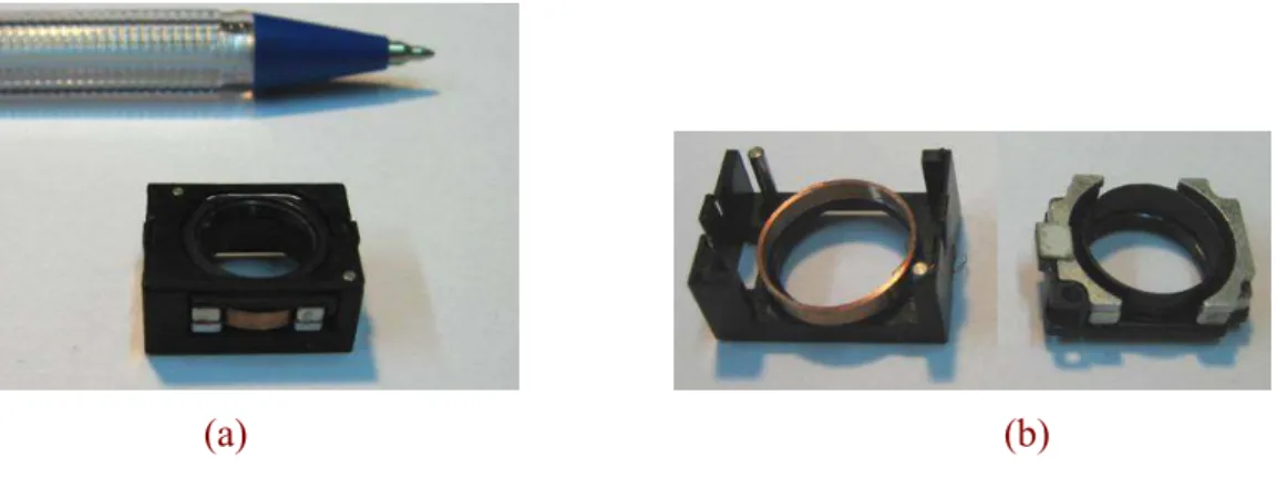
2.10 (a) Experiment model of the lens actuator, (b) stator and mover ...19

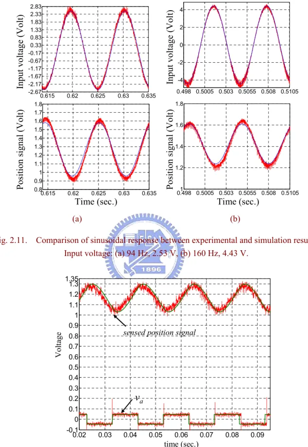
2.11 Comparison of sinusoidal response between experimental and simulation results. Input voltage: (a) 94 Hz, 2.53V, (b) 160 Hz, 4.43V. ...20

2.12 Comparison of step response between experimental and simulation results. Input square wave: 50Hz, 100 mV. ... 20

2.13 Comparison of impulse response between experimental and simulation results. Impulse time: (a) 1 ms, (b) 2 ms, (c) 3 ms. ...22

3.1 Block diagram of the proposed digital control scheme. ...23

3.2 Full-bridge converter used in the current loop. ...24

3.3 Block diagram of the simplified current loop...26

3.4 The current loop bandwidth is designed to be 10k Hz: (a) loop gain, (b) closed loop frequency response...27

3.5 FFT of the inductor current under several different fcs...29

3.6 Simulation of the current loop sinusoidal response...30

3.7 Simulation of the current loop step response. ...30

3.8 Block diagram of the velocity loop ...31

3.9 Block diagram of the position loop ...32

3.10 Simulation of position response under several different

ε

. ...34 3.11 (a) Simulation of the position and velocity response, (b) current response for

3.12 (a) Simulation of the position and velocity response, (b) current response for

a small position command change...36

4.1 Schematic of the prototype lens module servo control system. ...37

4.2 Experimental setup for the lens module servo control system ...38

4.3 Pin assignment of the constructed servo control IC ...39

4.4 Timing analysis of the ALU sharing effort ...40

4.5 Block diagram of the ALU ...40

4.6 Experimental results of the current loop step response: (a) 25%, (b) 50%, (c) 75% of the maximum current ...42

4.7 Transient of the current loop step response: (a) 30 mA, (b) 60 mA, and (c) 90mA ...43

4.8 Experimental results of the position and current response, 90% of the full stroke: (a) the lens module moves up-and-down, (b) the transient response ...44

4.9 Experimental results of the position and current response, 15% of the full stroke: (a) the lens module moves up-and-down, (b) the transient response ...45

Chapter 1

Introduction

1.1. Research Background and Recent Development

In recent years, mobile phones have been evolved to a development trend to integrate almost every digital media function, such as MP3, voice recorder, digital camera, broadband radio, and even digital TV. At the same time, a mobile phone is also required to be more lighter, thinner, and longer usage time, this means lower power consumption and efficient dynamic power management is a must. Auto-focus is a fundamental requirement for a digital camera or a video recorder. In the conventional approach, the auto-focusing is accomplished via a stepping motor with open-loop control. This solution has disadvantages of low control resolution, possible losing steps for fast image tracking, large volume, and large power consumption for its continuous winding excitation. Because of these disadvantages, voice coil motor (VCM) is one of many promising candidates for next generation digital cameras.

The VCM is evolved from the principle of a loudspeaker in vibrating its diaphragm by exciting its voice coil with a controlled current. Therefore, the VCM is used in applications of linear positioning control systems with small control range, such as an optical read/write head of DVD or an auto-focus module of a digital camera. In recent marketing, the VCM in applications for camera lens actuator use spring in return to achieve open-loop position control [1]. The mechanism is hard to assemble and consumes much power especially when large displacement due to the elastic force, thus it is not a good solution.

On the other hand, due to the development of microcontrollers, the different control loops have changed from analog to digital implementation, which allows more advanced control features. The analog approach (based on op-amps, resistors and capacitors) does not easily allow change of control parameters and noise may limit the performance. However, the bandwidth of analog controllers can be made very high. The advantage of digital programmable controllers is that the control parameters are easily changed. Field- programmable-gate-arrays (FPGA) now offer sufficiently high gate-density on a single IC that the flexibility of digital software controllers can be realized in hardware.

1.2. Research Motivation and Objectives

The VCM designed in this thesis needs no spring in return. It is composed of a coil and two yoke plates (top and bottom) where permanent magnets are bonded in a fixture. Its operation principle follows the Lorentz force law and it offers the advantages of simple and rigid structure, fast response, no cogging force, no force ripples, and can be controlled with high accuracy. The design issue resides in how to arrange a fixed volume of the magnet within a restricted volume to achieve the largest force constant [2]-[4] and at the same time to lower its power dissipation [5]. In additional to the energy saving and minimum volume requirements, fast dynamic response and high accuracy are also required for the positioning control of the VCM module [6]. Therefore, an iterative optimal design process is proposed to maximize the force constant of the VCM with a specified volume. In order to achieve this optimization-oriented design goal, an accurate model of the VCM is important both for the motor design and the servo control chip design. Thus a modeling procedure for the specially designed VCM is developed based on its mechanical structure and used material by using an electromagnetic simulation software—the Ansoft’s Maxwell 2D.

This thesis also presents a systematic solution that integrates the slim-type VCM and the dedicated digital servo control IC for the auto focus lens module in applications to high performance mobile phone camera. The servo control IC is composed of two parts—the controller and the power drive circuit. The former adopts fully digital control scheme, in which the highest sampling frequency is 200 kHz. The latter uses a full-bridge dc-dc converter as the power amplifier, and the switching frequency is 100 kHz. The controller generates PWM signal directly and thus no D/A converter is needed. The DC link voltage is 3.3 V and the maximum output current is 120 mA. This thesis presents the design and modeling procedure of the VCM and proposes the design scheme of each control loop of the digital servo drive IC. The design is implemented by FPGA and the experimental results are verified that the AF lens module can reach a control range of 0.6 mm within 30 ms with a control resolution less than 30 µm. Therefore, the design can achieve the requirement of low power consumption, high resolution and fast response.

1.3. Thesis organization

The thesis is organized as follows. In chapter 2, the fundamentals and the mathematical modeling of the voice coil motor is introduced, and the optimal design procedure is presented. Simulation results with experimental verification show the closeness of the mathematical model and the physical model.

In chapter 3, the design methodology to implement a fully digital control IC for the position control of the VCM in applications to auto-focus lens module of mobile phone camera is presented. Simulation analyses are also given in this chapter.

In chapter 4, the laboratory setup of the auto-focus lens module drive is introduced, and the FPGA-based implementation issue is discussed. The overall performance is verified through experimental results. Some concluding remarks related to this research are summarized and discussed in Chapter 5.

Chapter 2

Modeling and Design of the Voice-Coil Motor

2.1. Magnetic-Field Analysis

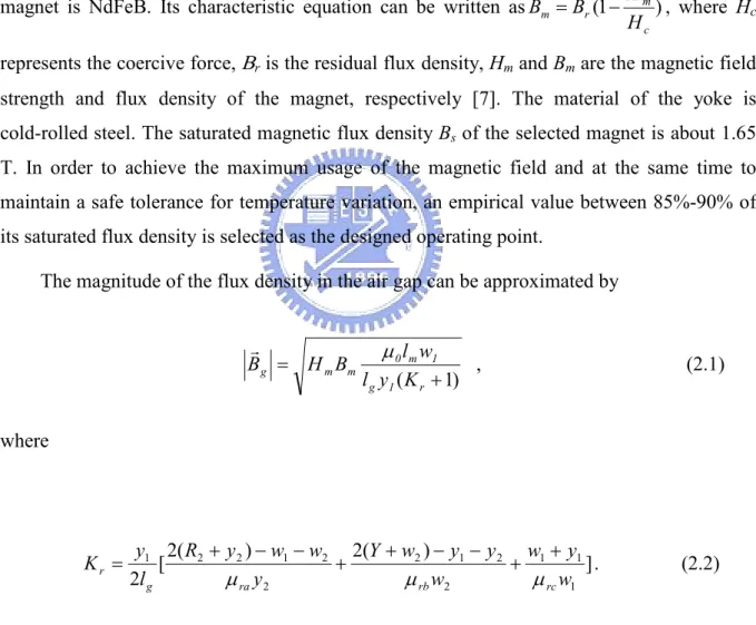
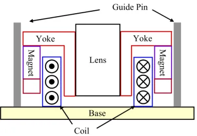
Fig. 2.1 shows the cross-sectional structure of the VCM used for auto-focusing control of the lens for a digital CCD camera and Fig. 2.2 illustrates its defined design parameters. The permanent magnetic circuit includes a magnet, two yokes, and the air gap. The material of the

magnet is NdFeB. Its characteristic equation can be written as (1 )

c m r m H H B B = − , where Hc

represents the coercive force,

Β

r is the residual flux density, Hm and Bm are the magnetic field strength and flux density of the magnet, respectively [7]. The material of the yoke is cold-rolled steel. The saturated magnetic flux density Bs of the selected magnet is about 1.65 T. In order to achieve the maximum usage of the magnetic field and at the same time to maintain a safe tolerance for temperature variation, an empirical value between 85%-90% of its saturated flux density is selected as the designed operating point.

The magnitude of the flux density in the air gap can be approximated by

) 1 ( + = r 1 g 1 m 0 m m g K y l w l B H B

µ

r , (2.1) where ] ) ( 2 ) ( 2 [ 2 ₁ 1 1 2 2 1 2 2 2 1 2 2 1 w y w w y y w Y y w w y R l y K rc rb ra g r

_µ

_µ

_µ

+ + − − + + − − + = . (2.2)

If yoke A, yoke B, and yoke C work on the same operation point, their relative permeability

µ

ra =

µ

rb =

µ

rc. The VCM’s operation principle follows the Lorentz force law:

dV B J F V g c

∫

× = r r r , (2.3)

Base Lens Yoke M ag n et Yoke Guide Pin M ag n et Coil

Fig. 2.1. The structure of the mobile phone camera.

360˚ d_m l_g y₂ y₁ l_m Y R₁ w₂ wc w₁ y_c S N Yoke A Yoke C Coil R_{2 r} z Y o k e B

where Jc is the current density and V represents the volume of the coil. The average length per

winding lc is approximately π(2R1+ 2w2 + lg ). Let Bgr be the quantity of Bg

v

in the r-direction on the central of the air gap. Assume that the current density is uniform distributed, and Bgr is

uniform distribution in the r-direction since the width of the air gap is very small. The magnitude of F v in the z-direction: dz z B l D l i K i F c m m d y d gr c g a F a m 2

∫

( ) + ⋅ ⋅ ⋅ = ⋅ = , (2.4)

where ia is the motor current and D is the diameter of the coil. Let the operation point of the

magnet be its maximum energy product that generates larger flux density in the air gap. Enlarging w1 will increase Bg

v

. However, if lg is suppressed, then less windings are included.

If w2 is suppressed, then yoke B becomes saturated. Both the conditions decrease KF. On the

other hand, increasing lm makes yoke A or yoke C become saturated, thus Kr is increased, and

g

B v

is decreased so that KF is reduced. Therefore, a design procedure must be constructed to

decide how to arrange a fixed volume of magnet within a restricted volume to achieve the largest force constant.

2.2. Features of Maxwell 2D

Maxwell 2D is the electromagnetic simulation software program that helps users develop

virtual prototypes of electric machines, actuators, transformers, and other electromagnetic

devices that can be represented in two dimensions. Maxwell 2D includes five solver modules:

Transient, AC Magnetic, DC Magnetic, Electric Field, and Thermal. The modules are

designed to solve problems in the static, frequency, and time-varying electromagnetic

domains, including motion and thermal coupling. Each module uses the 2D Finite Element

Method (FEM), tangential vector finite elements, and automatic adaptive meshing techniques

to compute the electrical/electromagnetic behavior of low-frequency components. With

Maxwell 2D, users solve for electromagnetic-field parameters, such as force, torque, and

impedance, as well as generate state-space models, visualize 2D electromagnetic fields, and

optimize design performance [8].

This thesis adopted the DC Magnetic solver module of Maxwell 2D and the function of

geometric parameter sweep during parametric analysis. The DC Magnetic solver module

computes static magnetic fields where the source originates from a DC current or voltage,

permanent magnets, or externally applied magnetic fields. The properties of the materials can

be linear, nonlinear or anisotropic. The simulation results show the magnetic force or torque

applied to the designate object, inductance of the windings, stored energy and visualization of

magnetic fields.

The parametric analysis module breaks a Maxwell 2D project down into two parts: a

nominal model and a parametric model. The nominal model is created like any other 2D

model, except that the design parameters which will be changed during a parametric sweep

must be defined as variables while drawing the geometry, assigning material properties, and

properties, or functional boundary/source quantities are assigned the values that specified

while setting up the parametric sweep. The number of variations that can be defined for a

parametric model is limited only by computation resources. The simulation results obtained

for each setup can be compared to determine how each design change affects the model

performance.

In this thesis, the geometric parameters y1, y2, w1 and w2 in Fig. 2.2 are set to be swept

during parametric analysis. The simulation results show the magnetic field distribution and

the magnetic force on the mover of the VCM. The statistical data can be used in the optimum

design procedure.

2.3. Optimum Design Procedure

Let KF be the objective function and assume that yc = y1 + lm and the gap between the

coil and the yokes is very small, i.e. l ≈_g w_c. The optimization problem is described as follows: Maximize dz z B l D l f c m m d y d gr c g obj 2

∫

( ) + ⋅ ⋅ = (2.5) subject to 2 2 1 w l R w + + _g = , (2.6) Y l y y₁+ ₂ + _m = , (2.7)

where R1, R2 and Y are fixed numbers according to the dimensions specification of the lens module.

The objective function has four independent variables y1, y2, w1 and w2. Under the constraint, by sweeping every possible combination of the variables, one can find the solution. However, this is time consuming. The flow chart that using Ansoft’s Maxwell 2D to solve the

problem is shown in Fig. 2.3. The first half of the flow chart is the standard steps to construct a model with definition of geometric variables. After the environment is set up, let W = (w1, w2) and Y = (y1, y2). Select an initial value of Y, named Y0, and sweep W, until the maximum value of fobj(W0) under Y0 is present. Next, fix W = W0 and sweep Y until the maximum value of fobj(Y1) under W0 is present. If the two values of fobj are equal or in the range of

calculation error, the solution is converged. Otherwise, the algorithm finds the next value of fobj to compare with the one before.

Define Model & Define Variables Setup Materials Select Boundaries & Sources Define Items to Be Solved Setup Solution

Select an initial value of Y

Defined the Sweep Range and Step Size

Fix Y_n, sweep W, Find f_obj,m(W_n,Y_n) f_obj,m(W_n,Y_n+1) > f_obj,m(W_n,Y_n) ? Fix W_n, sweep Y, Find f_obj,m(W_n,Y_n+1)

Find the maximum of f_obj,m(W,Y) m = K ? Yes No No Yes START END n = n+1 m = m+1

This method takes much less calculation time than sweep every combination of the four variables. However, it doesn’t guarantee to find out the global maximum, thus the outer loop of the flow select K different initial value to compare with one another. Larger K takes more computing resources, and increases the possibility to get the global maximum. Another tip to reduce the computing time is adding the two inequalities: y ≥₂ w₂ and y ≥₁ w₁, since flux leakage happens especially at the corner of the L-shaped steel and in the air gap.

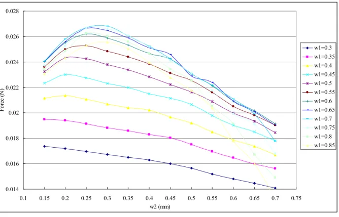
Let R1 = 4 mm, R2 = 2 mm, Y = 2.5 mm and the current density Jc = 2.8 A/mm2. Fig. 2.4

shows the simulation result of searching fobj,max using the flow mentioned above. Fig. 2.4(a) shows that at first, select Y0 = (0.3, 0.2), sweep W from (0.05, 0.05) to (0.8, 0.8). The simulation result shows that there exists a local maximum of Fm around W0 = (0.65, 0.25). This result is definitely to be modified in the next step since y2 < w2 is not reasonable.

In Fig. 2.4 (b), the solution is moved to W = W0 and Y1 = (0.5, 0.3), the magnetic force is about 26 mN, which is larger than the one in the first step. It also shows that if y2 is about 0.2 mm to 0.4 mm, increasing y1 from 0.05 mm to 0.5 mm tends to make more magnetic flux flow through the air gap so that the magnetic force is increased. When lm is suppressed less

than 1.2 mm, the flux density in the air gap falls extremely, thus the magnetic force is decreased. According to the simulation result, the maximum value of the magnetic force in this step is in the range of y2 = 0.2~0.4 mm. If y2 is too small, then yoke A becomes saturated. If y2 is too large, then the magnet is suppressed. Both the conditions decrease the flux in the air gap. Figs. 2.4(c) and 2.4(d) show that the solution is converged around W = (0.7, 0.3), Y = (0.5, 0.35), and the maximum magnetic force is 26.8 mN.

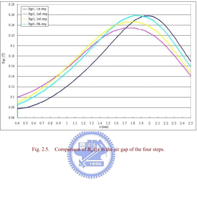
To show how the flux density is improved during the optimization process, Fig. 2.5 illustrates Bgr(z) on the central of the air gap of the four steps. Because the initial value of y1 in the first step is selected very small, the flux lines are gathered in the section of y1 and the flux density in the rest part of air gap is very low. In the second step, y1 is increased so that the flux is spread in a wider range. Next, w1 is increased and the permanent magnet generates more flux, thus the flux density in the air gap is increased. Finally, the solution is converged in the fourth step, and the distribution of flux density is Bgr4.

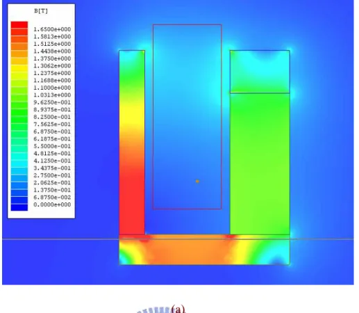
Figs. 2.6(a) and 2.6(b) show the distribution of the flux density and the flux lines, respectively. Since yoke B is a little thinner than yoke A, the magnetic density is about 1.5 T, which is near the magnetic saturation point. The flux density is under 1.3 T in yoke A and yoke C, thus no magnetic saturation occurs, the permeability is relatively high.

0 0.002 0.004 0.006 0.008 0.01 0.012 0.014 0.016 0.018 0.02 0.022 0.024 0.05 0.1 0.15 0.2 0.25 0.3 0.35 0.4 0.45 0.5 0.55 0.6 0.65 0.7 0.75 w2 (mm) F o rc e (N ) w1=0.05 w1=0.1 w1=0.2 w1=0.3 w1=0.4 w1=0.5 w1=0.6 w1=0.7 w1=0.8 (a) 0.01 0.012 0.014 0.016 0.018 0.02 0.022 0.024 0.026 0.028 0.05 0.1 0.15 0.2 0.25 0.3 0.35 0.4 0.45 0.5 0.55 0.6 0.65 0.7 0.75 0.8 0.85 0.9 0.95 1 1.05 y2 (mm) F o rc e (N ) y1=0.05 y1=0.2 y1=0.3 y1=0.4 y1=0.5 y1=0.6 y1=0.7 y1=0.8 y1=0.9

0.014 0.016 0.018 0.02 0.022 0.024 0.026 0.028 0.1 0.15 0.2 0.25 0.3 0.35 0.4 0.45 0.5 0.55 0.6 0.65 0.7 0.75 w2 (mm) F or ce ( N ) w1=0.3 w1=0.35 w1=0.4 w1=0.45 w1=0.5 w1=0.55 w1=0.6 w1=0.65 w1=0.7 w1=0.75 w1=0.8 w1=0.85 (c) 0.018 0.019 0.02 0.021 0.022 0.023 0.024 0.025 0.026 0.027 0.028 0.15 0.2 0.25 0.3 0.35 0.4 0.45 0.5 y2 (mm) F o rc e (N ) y1=0.4 y1=0.5 y1=0.6 y1=0.7 y1=0.8 (d)

Fig. 2.4. Searching process for fobj,max: (a) Y = Y0, search W for fobj,max(W0,Y0), (b) W = W0,

search Y for fobj,max(W0,Y1), (c) Y = Y1, search W for fobj,max(W1, Y1), (d) W = W1, search Y

(a)

(b)

Fig. 2.6. (a) The flux density of the optimized permanent magnetic circuit. (b) The flux lines of the optimized permanent magnetic circuit.

2.4. Modeling of the Lens Module

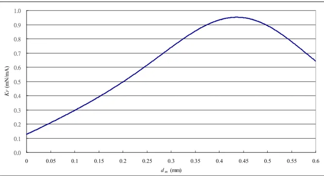
In a well designed motor, the torque (or force) constant is tuned to be a constant value for its rotating range. However, for a linear motor, especially a mall linear motor with very small transverse distance, limited space, and an aspect ratio close to unity, the resulted force may not be a linear function of the stator current due to a nonlinear flux linkage. According to the design procedure illustrated in the previous section, let Bgr4 be Bgr in (2.4), the force

constant KF is a function of mover position due to the changing coupling field as shown in Fig.

2.7. The minimum of KF is 0.128 mN/mA at dm = 0 mm, and the maximum is 0.952 mN/mA

at dm = 0.43 mm. The average value is 0.63 mN/mA.

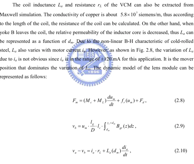
The coil inductance La and resistance rL of the VCM can also be extracted from

Maxwell simulation. The conductivity of copper is about 5 ×.8 107siemens/m, thus according to the length of the coil, the resistance of the coil can be calculated. On the other hand, when yoke B leaves the coil, the relative permeability of the inductor core is decreased, thus La can

be represented as a function of dm. Due to the non-linear B-H characteristic of cold-rolled

steel, La also varies with motor current ia. However, as shown in Fig. 2.8, the variation of La

due to ia is not obvious since ia is in the range of ±120 mA for this application. It is the mover

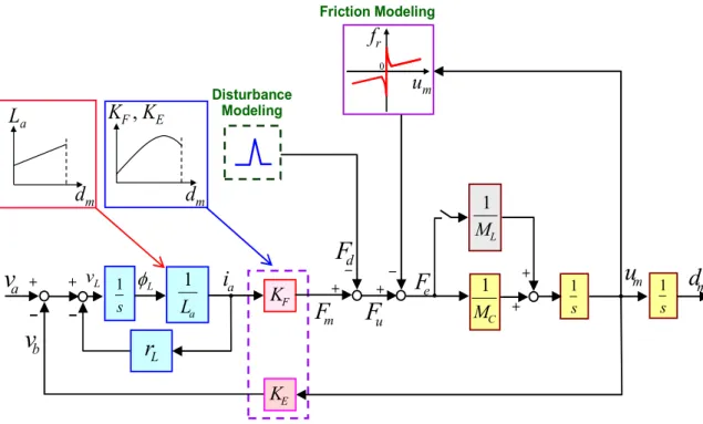
position that dominates the variation of La. The dynamic model of the lens module can be

represented as follows: d m r m L c m f u F t d u d M M F =( + ) + ( )+ , (2.8)

∫

+ ⋅ ⋅ ⋅ = c m m d y d gr c g m b l B z dz D l u v ( ) , (2.9) t d i d d L r i v v a m a L a b a − = ⋅ + ( ) , (2.10)

where Mc and ML are the mass of VCM and camera lens, respectively, vb is the back-EMF of

the VCM, and um is the velocity of the VCM. The variation of La due to ia is ignored in (2.10).

been characterized as nonlinear functions of mover position. The force constant reveals a large variation that can not be ignored even with a small range of motion and this is due to the large magnetic force resulted by the stator. The force disturbance comes from the weight of the module. When the module does not move horizontally, the weight of the module should be taken in to consideration. The friction modeling is the standard Coulomb plus static plus viscous friction model [9]-[10]. Let Fm – Fd be Fu and the stick region width be ±∆um, when

the lens is still, |um| < ∆um :

   ⋅ ≤ = ohterwise F f f F if F u f u s s u u m r ) sgn( | | ) ( , (2.11)

and when the lens is in motion, |um| > ∆um :

m B m c m r u f u K u f ( )= sgn( )+ , (2.12)

where fc > 0 is the Coulomb friction level, fs is the static friction force, and KB > 0 is the

viscous friction coefficient. These parameters are extracted from experiments.

TABLE 2.1

PARAMETERS OF THE TEST VCM

Parameter Value Unit

VCM inductor, L 410 mH

ESR of inductor, rL 25 Ω

force constant (averaged), KF 0.63 mN/mA

back-EMF constant (averaged), KE 0.63 V/mm/ms

mass of the mover, MC 0.3 g

mass of the lens, ML 0.7 g

maximum stiction force (with load), fs 5.9 mN

0.0 0.1 0.2 0.3 0.4 0.5 0.6 0.7 0.8 0.9 1.0 0 0.05 0.1 0.15 0.2 0.25 0.3 0.35 0.4 0.45 0.5 0.55 0.6 dm (mm) KF (m N /m A )

Fig. 2.7. Simulation derived force constant as a function of mover position.

0.35 0.36 0.37 0.38 0.39 0.40 0.41 0.42 0.43 0.44 0.45 0.46 0.47 0.48 0.49 0.50 -120 -100 -80 -60 -40 -20 0 _{20 40 60 80} 100 120 current (mA) in d uc ta nc e (m H ) ) dm=0 mm dm=0.1 mm dm=0.2 mm dm=0.3 mm dm=0.4 mm dm=0.5 mm dm=0.6 mm

_ m

u

m

F

d

F

a

v

+ −−−− a

i

a L 1 b

v

L

r

E K + −−−− KF e

F

Electro-to-Mechanical Power Conversion Disturbance Modeling s 1 L v φ_L s 1 C M 1 s 1 Friction Modeling

u

_m

f

_r 0 m

d

d

_m

K

_F

, K

_E

L

_a

d

_m + + _ + + L M 1 u

F

2.5. Error Analysis for the modeling of a VCM

A VCM is constructed based on the proposed design procedure. The experiment model of the lens actuator is shown in Fig. 2.10. The size of the module is10mm×14mm×4mm. The stator of the actuator consists of a set of coil and a pair of guide pin. The mover is composed of a pair of permanent magnet that bounded in two plates of yoke. A position sensor by using a non-contact photo transistor has been designed to convert the physical position 0-0.6 mm to 0.5-1.7 V. In order to verify its performance of the designed VCM and modeling accuracy, a set of sinusoidal voltage signals with different frequencies have been applied to the VCM. Fig. 2.11 shows the closeness of the measured experimental results with the block diagram based simulation results. It should be noted that the motor parameters are derived from the Maxwell 2D—a two-dimensional finite-element based electromagnetic simulation software. The parameters of the test VCM are shown in Table 2.1. Though the sinusoidal response of the experiment and simulation looks much alike at the two specific frequencies, it can not guarantee the accuracy of the mathematic model at every frequency. Thus the step response of experiment and mathematic model is tested. Fig. 2.12 shows that a square wave is applied to the VCM, and the position response of experiment and simulation are consistent. Furthermore, in order to excite the nonlinear behavior of the model, the comparison of the impulse response of experiment and mathematic model is shown in Fig. 2.13. The actuator is set to move up and down. It can be seen that in Fig. 2.13 (b), the position signal of experiment lags that of simulation during 25 ms to 30 ms. This phenomenon arises from the viscous friction of the experiment model larger than that of the simulation at that place. Thus a friction model that varies with displacement should be constructed.

(a) (b)

In

p

u

t

v

o

lt

ag

e

(V

o

lt

)

Time (sec.)

P

o

si

ti

o

n

s

ig

n

al

(

V

o

lt

)

0.615 0.62 0.625 0.63 0.635 -2.67 -2.17 -1.67 -1.17 -0.67 -0.17 0.33 0.83 1.33 1.83 2.33 2.83 0.615 0.62 0.625 0.63 0.635 0.8 0.9 1 1.1 1.2 1.3 1.4 1.5 1.6 1.7 1.8 0.498 0.5005 0.503 0.5055 0.508 0.5105 -4 -2 0 2 4

In

p

ut

v

o

lt

age

(

V

ol

t)

Time (sec.)

Po

si

ti

on

s

ig

n

al

(

V

o

lt

)

0.498 0.5005 0.503 0.5055 0.508 0.51051 1.2 1.4 1.6 1.8 (a) (b)

Fig. 2.11. Comparison of sinusoidal response between experimental and simulation results. Input voltage: (a) 94 Hz, 2.53 V, (b) 160 Hz, 4.43 V.

0.02 0.03 0.04 0.05 0.06 0.07 0.08 0.09 -0.1 0 0.1 0.2 0.3 0.4 0.5 0.6 0.7 0.8 0.9 1 1.1 1.2 1.3 1.35 time (sec.) sensed position signal

v

_a

V

ol

ta

ge

Fig. 2.12. Comparison of step response between experimental and simulation results. Input square wave: 50 Hz, 100 mV.

0 0.01 0.02 0.03 0.04 0.05 -0.5 0 0.5 1 1.5 2 2.5 3

Time (sec.)

V

o

lt

sensed position signal

v

_a (a) 0 0.01 0.02 0.03 0.04 0.05 -0.5 0 0.5 1 1.5 2 2.5 3

Time (sec.)

V

o

lt

sensed position signal

v

_a

0 0.01 0.02 0.03 0.04 0.05 -0.5 0 0.5 1 1.5 2 2.5 3

Time (sec.)

V

o

lt

_{sensed position signal}

v

_a

(c)

Fig. 2.13. Comparison of impulse response between experimental and simulation results. Impulse time: (a) 1 ms, (b) 2 ms, (c) 3 ms.

Chapter 3

Design and Analysis of the Voice-Coil Motor Servo

Control IC

The design of VCM in this thesis is composed of a set of permanent-magnetic circuit and coil. Its operation principle follows Lorentz force law. Instead of using spring-return method, the lens’ motion is under closed loop control. Therefore, compared with the mechanism that with spring in return, the holding power is lowered and the ringing phenomenon does not exist. The size of the lens module is 10mm× 14mm × 13mm and the mass of the mover with lens is 1 g.

The proposed VCM servo control IC provides total digital solution for fast auto focus mobile phone camera applications. As shown in Fig. 3.1, the driver stage uses a full-bridge dc-dc converter as the power amplifier, and the switching frequency is 100 kHz. The DC link voltage is 3.3V and the maximum output current is 120 mA. The settling time is less than 30 ms with a control resolution less than 30 µm. Therefore, the design can achieve the requirement of low power consumption, high resolution and fast response.

2nd order IIR Filter L r Ls + 1 f K s 1 + - Ms 1 F_pin + + f ( v, po) Mg + ₊ PWM K cf K + -e K 2 s T pf K lv K Velocity Estimator + - + -+ 1 1− z− Kic pc K + + pcmd po i_o v_o icmd vcmd

Digital Controller Physical System and Feedback Filter

Anti-alias Filter v back-EMF non-linear position loop gain 2 s T 1 s T p_fbk perr v_est v_err i_fbk

3.1. Current Loop Design

V_dc T_A+ T_A -T_B+ T_B -L r_L back-EMF Digital PWM Current Loop Controller cf K 2 s T PWM0~ PWM3 +-i_cmd i_o i_fbk

Fig. 3.2. Full-bridge converter used in the current loop.

Fig. 3.2 shows the current driver is realized by a digital control loop, in which the driver stage is a full-bridge converter. The digital pulse width modulator generates switch control signals by means of unipolar voltage switching.

Compared with bipolar voltage switching, under the same switching frequency, unipolar has less output current ripple. The amplitude of the current ripple is:

L DT D V i_L = _d( −1 ) _s/4 ∆ . (3.1)

When D = 0.5, ∆i_L reaches the maximum value, named∆i_L,max . The switching frequency is 100 kHz so that ∆i_L,max is less than 5% of the maximum motor current, i.e.

L d

L V r

i _,max ≤0.05 /

∆ .

The main advantage in using a current driver is to fasten the response. On the other hand, the current through the VCM is insensitive of variations in winding impedance and back-EMF. The back-EMF can be viewed as a disturbance in the current loop. The transfer function Gc (s)

2 2 ) ( e L c K Ms r MLs Ms s G + + = . (3.2)

In this application, the VCM has small inductance and relatively large equivalent series resistance (ESR), thus

M K L

r_L2 4 _e2

>> . (3.3)

The transfer function Gc (s) can be reduced to

L c r sL s G + ≈ 1 ) ( . (3.4)

In order to improve dynamic response, the bandwidth of current loop can be extended with pole-zero cancellation to speed up the response time. Therefore, a PI controller is applied and the current-loop bandwidth is decided by the controller gain. Let i_e[k]=i_cmd[k]−K_cf ⋅i_o[k], the current-loop control low is designed as

] 1 [ ] 1 [ ] [ ) ( ] [k = K +K i k +K i k− +v k− v_{c ic pc e pce c} , (3.5) cf PWM c pc K K L K K = 2

π

, (3.6) cf PWM sc L c ic K K f r K K = 2

π

, (3.7)

where fsc is the sampling frequency of the current-loop controller and Kc is the controller gain

that decides current-loop bandwidth. However, the switching frequency of the full-bridge converter is 100 kHz, according to sampling theorem, the current-loop bandwidth can not lager than 50 kHz. Actually, in addition to the limitation of the switching frequency, the

-+ i_o ±V_d L r sL + 1 1 s T tri d V V ˆ 1 1− z− Kic pc K + + c K G_c(z) ZOH G_h(s) digital controller cf K Calc. Delay Calc T i_fbk i_cmd v_o

Fig. 3.3. Block diagram of the simplified current loop.

sample-and-hold and calculation delay also add limitation to bandwidth. The block diagram of the simplified current loop is shown in Fig. 3.3. The phase delay caused by sample-and-hold and calculation at the gain crossover frequency Fc is represented as:

Calc c s c Calc H S d F T T F × + °× × × ° = + = 360 2 360 1 / φ φ φ , (3.8)

and the phase margin φ_m = 90°−φ_d. Approximate the phase response by the second order system, the relation between φ_m and damping ratio ξ is

        − + = − 0.5 2 4 1 ) 2 1 4 1 ( 2 tan

ξ

ξ

ξ

φ

m . (3.9)

Assume that the calculation time of the digital controller is 2.5 µs and Ts1 is 10 µs, from (3.8), °

= 27

d

φ . If little overshoot is allowed in the close loop step response, select ξ =0.7, and from (3.9), φ_m = 65°. Fig. 3.4(a) shows the gain crossover frequency is designed at 10 kHz and the phase margin is 65°. The current loop bandwidth is about 10 kHz as shown in Fig. 3.4(b).

=65˚

m

φ

(a)

(b)

Fig. 3.4. The current loop bandwidth is designed to be 10 kHz; (a) loop gain, (b) closed loop frequency response.

In a digital control loop, there should be appropriate proportional relation among sampling period, quantification, and bandwidth. Sampling period represents the division on the horizontal axle (time) while quantification represents the division on the vertical axle (magnitude). Too much the bit length or too fast the sampling frequency expends system resources, or conversely, leads to distortion of signal. Let the frequency f_t and the amplitude A_t of the test sinusoidal wave be

m f f s t 2 = , (3.10) 1 2 / − = d_n t R V m A , (3.11)

where fs is the switching frequency, n is the bit length and m is an integer. According to the

previous design, the current loop bandwidth is 10 kHz and fs is 100 kHz, thus m = 5. Consider

the working point at the maximum common used current, 70 mA, according to (3.1), the amplitude of the current ripple is 5.25 mA. Let the amplitude of the test sinusoidal wave at this working point be at least larger than 5.25 mA, according to (3.11), the bit length of the digital controller output n = 8. Because the converter uses unipolar voltage switching scheme, the equivalent switching frequency is 200 kHz, the command rate of the current controller output fcs is 200 kHz. Fig. 3.5 shows the harmonics of the inductor current under several

different fcs. It is obvious that if fcs is select to be 2fs, then there is no harmonic other than the

fundamental frequency and the even-numbered harmonics due to switching frequency, which means lower THD.

Table 3.1 shows the comparison of THD under several different bit lengths: 6-bit, 8-bit, and 10-bit, in which fcs = 2fs = 200 kHz. The THD of n = 6-bit is 35.88%, which is about three

times larger than that of n = 8-bit. Though the THD of n = 10-bit is lower than that of n = 8-bit, the difference is less than 2%, which can be ignored.

Let the working point be 70 mA, Fig. 3.6 shows the current loop provides good tracking ability for a 10 kHz, 5.5 mA sinusoidal command. Next, the step response is also tested. As shown in Fig. 3.7, the step commands are 20 mA, 40 mA, and 50 mA. The rise time tr is about

f_cs=f_s/ 2=50 kHz

f_cs=f_s=100 kHz

f_cs=2 f_s=200 kHz Unipolar Voltage Switching

50kHz 100kHz

150kHz

Fig. 3.5. FFT of the inductor current under several different fcs.

TABLE 3.1

THDUNDER SEVERAL DIFFERENT BIT LENGTHS

Bit Length THD

6-bit 35.88%

8-bit 11.5%

i

_cmd

/ K

_cf

i

_L

(A)

Fig. 3.6. Simulation of the current loop sinusoidal response.

35 µs i_L(A)

70 m

Saturation

3.2. Servo Loop Design

3.2.1. Velocity Loop

cf K 1 3 s T pf K lv K Velocity Estimator T_s3 ZOH _s 1

-v

_cmd

+

p

_o

current

loop

Ms 1 f K

+

+

force

disturbances

v

_est

G

_h3

(s)

i

_cmd

v

Fig. 3.8. Block diagram of the velocity loop.

Since the position signal is present in the digital controller, a numerical method is used to estimate the motor speed. The velocity estimator is implemented using the second-order Taylor series expansion [11]:

)] ( 2 / 1 [∆ + ∆ −∆ ₋₁ = _{D k k k} est K x x x v , (3.12)

where v_est is the estimated velocity during k-th period, ∆xk and ∆xk-1 represent measured position change during k-th and (k-1)-th sampling interval. As Fig. 3.8 is shown, Kpf is the

position sensor gain. The velocity feedback acts when the transient of the position response and rests when the lens module is in position. The velocity controller gain Klv is decided by

D pf f cf cv lv K K K MK K =

ω

, (3.13)

where ωcv is the velocity loop bandwidth that is proportional to Klv. The zero order hold (ZOH)

models the delay of the discrete sampling time of the velocity controller. The transfer function Gh3(s) of the ZOH is:

2 / sT −

The velocity estimator’s and ZOH’s contribution to the phase can be represented as: 3 3 , ZOH , 180 2 360 ) ( ) ( _{dvest s s} d vd T f T f f f + = °× × + °× × =

φ

φ

φ

, (3.15)

where f is the frequency of interest. Therefore, the velocity loop bandwidth is limited by the discrete time sampling delay of the digital controller. Let the sampling frequency of the velocity loop be 40 kHz, i.e., Ts3= 25 µs and the bandwidth of the velocity loop be 2.5 kHz, and then

φ

_vdon the gain crossover frequency is 11.25∘. The phase margin is about 79∘, which satisfy the stability. In fact, the mover of the VCM is so light (1 gw) such that the audible noise is a severe problem. Based on the experiments, ωcv is designed at 800 Hz to 1

kHz. Since the current-loop bandwidth is designed at 10 kHz, the current loop can be viewed as a DC gain 1/Kcf while designing the velocity loop.

3.2.2. Position Loop

D pfK K 1 3 s T pf K 3 s T ZOH s 1

-pcmd

+

po velocity loop look-up table p_fbk perr vcmd v

G

_h3

(s)

Fig. 3.9. Block diagram of the position loop.

Fig. 3.9 shows that the position controller is a look-up table that has higher gain when the position error is small and lower gain when the position error is large. The output of the controller is velocity command which is defined as

     − < ∆ ⋅ − ⋅ < ∆ ⋅ + ⋅ ≤ ⋅ =

ε

ε

ε

ε

ε

err p err p err p err p err err p cmd p if K p K p if K p K p if p K v 2 2 1 , (3.16)

where ∆Kp = Kp1 - Kp2, Kp1and Kp2 are the controller gain of different region of the position error defined by ε. Appling higher gain at low position error makes the controller generate larger current command to overcome the force disturbances such as the weight of the lens (Mg), guide pin magnetic force (Fpin(po)), and static friction (fs) when the VCM is beginning

to move. The higher gain Kp1 also reduces position steady state error since no integrator is present in the servo loop controller. The reason that not using an integrator is to prevent the system suffers from stick-slip oscillation. The steady state position error produced from Mg and Fpin(po) is f lv p o pin ess K K K I p F Mg P p 1 max max 2 ) ( + = , (3.17)

where Imax is the maximum motor current and Pmax is the full stroke of the lens module. It can be seen that the parameters Pmax, Imax and Kf are fixed by motor specification, and Klv is

restricted by audible noise consideration, thus Kp1 is the major parameter designed to reduce steady state position error. However, rising Kp1 may introduce system oscillation, thus Kp2 is designed to make the position response have more following error to prevent system from oscillation. The following error eflv under this variable position loop gain is

) ( _{2 1} 1 2 fl fl fl fl flv e e e e e = −

ε

− , (3.18)

where efl1 and efl2 are the following error under constant position loop gain Kp1 and Kp2, respectively. The position loop bandwidth BWp is equal to 1/eflv, thus ε can be decided by the

specified BWp. Let Kp1 = 40, Kp2 = 10, Fig. 3.10 shows how the parameter

ε

affects the position response. The test position command pcmd is given in the bandwidth of position loop

so that the position response follows the command. When

ε

= efl1, according to (3.16) the following error eflv = efl1, i.e., the controller gain is equivalent to Kp1. When

ε

is decreased, the following error is increased, and the equivalent bandwidth is lowered. When

ε

= 0, the equivalent controller gain is Kp2.

0.02 0.022 0.024 0.026 0.028 0.03 0.032 0.034 2000 2200 2400 2600 2800 3000 3200 3400 3600 3800 4000 p_fbk2: ε=100 p_fbk3: ε=40 p_fbk4: ε=20 p_fbk1: ε=e_fl1 p_fbk5: ε=0 p_fbk3 p_fbk4 p_fbk5 p_fbk1 p_fbk2 p_cmd

Fig. 3.10. Simulation of position response under several different

ε

.

3.3.

Simulation Results and Analysis

Figs. 3.11 and 3.12 illustrate the position, velocity, and current response of a large and small position command change, respectively. In Fig. 3.11(a), the magnitude of the step change is about 90% of the full stroke. The mover is in-position in 30 ms that meets the specification. The range of the estimated speed is -2048~ 2047 which is mapped to

±80 µm/ms. Fig. 3.11(b) illustrates the current response. For saving simulation resources, the linear model of the current loop is adopted since the current loop bandwidth is much higher than the outer loops. According to the position and velocity response, during most of the transient, the mover is in uniform motion. However, the average of the current is not kept in constant. It is resulted from the non-linearity of the force constant, which is modeled as a function of mover position in section 2.3.

In order to overcome the static friction, extra force is needed when the mover is beginning to move, and the static friction becomes zero as long as the mover starts. Therefore, there is a little oscillation at the starting of the mover. This phenomenon affects the performance especially when the change of position command is small as shown in Fig. 3.12(a). One way to decrease the overshoot is to lower the slop of the ramp command when a small position commend is taken place. The steady-state error is about 2% of the full stroke that meets the specification, and no stick-slip limit cycle is present.

0.02 0.04 0.06 0.08 0.1 0.12 -1000 -500 0 500 1000 1500 2000 2500 3000 3500 4000 time (sec.) po si ti on c om m and, f ee d b ac k a nd est im at ed sp ee d ( di g it ) estimated speed position feedback position command (a) 0.02 0.04 0.06 0.08 0.1 0.12 -0.1 -0.08 -0.06 -0.04 -0.02 0 0.02 0.04 0.06 time (sec.)

m

o

to

r

cu

rr

en

t

(A

)

(b)

Fig. 3.11. (a) Simulation of the position and velocity response, (b) current response for a large position command change.

0.02 0.025 0.03 0.035 0.04 0.045 0.05 2500 2550 2600 2650 2700 2750 2800 2850 2900 2950 3000 time (sec.) p o si ti o n c o m m an d , fe ed b ac k ( d ig it ) position feedback position command 0.02 0.025 0.03 0.035 0.04 0.045 0.05 -1500 -1000 -500 0 500 1000 1500 time (sec.) es ti m at ed v el o ci ty ( d ig it ) (a) 0.02 0.025 0.03 0.035 0.04 0.045 0.05 -0.08 -0.06 -0.04 -0.02 0 0.02 0.04 0.06 0.08

m

o

to

r

cu

rr

en

t

(A

)

time (sec.) (b)

Fig. 3.12. (a) Simulation of the position and velocity response, (b) current response for a small position command change.

Chapter 4

Hardware Realization and Experimental Results

In order to verify the effectiveness of the developed servo control strategy, an FPGA-based drive system is setup for the experiments. In this chapter, the laboratory setup is first introduced. Then, the practical realization issues of the control IC are discussed.

4.1. Laboratory System

Fig. 4.1 illustrates the hardware architecture of the experimental system constructed in this thesis. The developed servo control IC works as a coprocessor with a single-chip MCU (AT89C51RD2) from ATMEL. The MCU serves as a host processor and governs the work of tuning control parameters. The developed servo control IC receives sensed position signal and inductor current from the lens module. The feedback signals are multiplexed before feeding into the 12-bit A/D converter. The position sensor maps the physical position 0-0.6 mm to 1.2-2.5 V, and the motor current is between ±120 mA. The converted digital data is then sent to FPGA for further processing. The experimental setup is shown in Fig. 4.2.

Control IC

MCU

VCM with

a Camera Lens

and a Position

Sensor

ADIN SCK SDA V+ V-SCK SDA

sensed position signal

sensed inductor current

EEPROM

DONE CCLK DIN

ADC

CONVST

Mux

12 RS232

Lens Module

FPGA Board

MCU Board

Power Supply

PC

4.2. Implementation of the VCM Servo Control IC

Fig. 4.3 shows the interface and functional block diagram of the constructed servo control IC for the VCM lens module. This IC allows user to set the controller parameter according to the load (camera lens) and response time. All modules including current controller, position filter, position controller, velocity estimator and velocity controller share the same ALU unit by time-sharing scheme for arithmetic operation. The time-sharing scheme is mixed with 40 kHz and 200 kHz sampling frequency as shown in Fig. 4.4.

Fig. 4.5 shows the detail block diagram of the ALU unit, which supports both of add, minus and single cycle operation for arithmetic operation a×b+c.

A/D Converter Position Controller Velocity Controller Current Controller Position Filter Velocity Estimator ALU System Manager Position Profile Generation _{40k Hz} 40k Hz 40k Hz 200k Hz 200k Hz 200k Hz 12 12 12 12 12 12 12 12 12 12 12 12 12 12 12 12 12 4 4 12 12 12 12 Full Bridge Converter 12 12 Register File I2_C Module 12 PIN IIN SCK SDA V+ V-12 12 200k Hz

Current

Controller

Position

Filter

Position

Controller

Velocity

Estimator

Velocity

Controller

5µ

25µ

5µ

5µ

5µ

5µ

time (sec.)

Fig. 4.4. Timing analysis of the ALU sharing effort.

Multiplier 1 0 Reformation Adder Shifter 2’s complement 1 0 mult_a [11:0] mult_b [11:0] mult_insigned mult_o [23:0] add_o [23:0] sub_add_a [11:0] mac_en shift_ref sub_add_b[11:0] sub_en shift_add [3:0]

4.3. Experimental Results and Analysis

To verify the design of the digital control IC, the current loop step response is first tested. In order to capture the waveform of current command and current response at the same time, the two digital signals are sent to D/A converter and the voltage signals are shown in Fig. 4.6. The maximum current is limited at 120 mA and the current commands are 25%, 50%, and 75% of the maximum current, respectively. The transient of current loop step response is shown in Fig. 4.7. It can be seen that the period of the current ripple is 5 µs. For unipolar voltage switching scheme, the switching frequency is 100 kHz. The rise time tr is defined as

the time required for the current changes from 10% to 90% of its final value. The current loop bandwidth BWc≅0.35/tr=10 kHz, which is consistent with the simulation results in section

3.1.

Fig. 4.8 illustrates the trapezoidal position response of the VCM with the designed digital servo drive IC, in which pcmd and pfbk are position command and position feedback,

respectively. The transverse distance is 0.54 mm with a feed rate of 20 µm/ms and can achieve a position control resolution of 30 µm. The magnitude of holding current at the lower position is 10 mA while that at the higher position is 40 mA. The magnitude of the peak current during the period is 60 mA, which is 50% of the maximum current. Compare the position and current response of Fig. 4.8 with that of Fig. 3.11, the experimental and simulation results are closed to each other. Next, a smaller change in position command is given. The slope of the ramp command is 20 µm/ms, the same as before. The magnitude of the position command is 0.09 mm, i.e. 15% of the full stroke. The magnitude of the peak current during one period is about 80 mA, which is 67% of the maximum current. Compare the position and current response of Fig. 4.9 with that of Fig. 3.12, the experimental and simulation results are consistent. Experimental results verify the designed digital servo drive IC can meet the design specifications of an auto-focus module used for high-performance slim-type digital camera applications.

i_cmd i_fbk (a) i_cmd i_fbk (b) i_cmd i_fbk (c)

Fig. 4.6. Experimental results of the current loop step response: (a) 25%, (b) 50%, (c) 75% of the maximum current.

t

_r

= 35 µs

(a)

t

_r

= 35 µs

(b)

t

_r

= 35 µs

(c)

i

_o

p

_fbk (a) p_cmd p_fbk p_fbk i_o i_o p_fbk p_cmd p_fbk (b)

Fig. 4.8. Experimental results of the position and current response, 90% of the full stroke: (a) the lens module moves up-and-down, (b) the transient response.

i

_o

p

_fbk (a) i_o p_fbk p_cmd pfbk i_o p_fbk p_cmd p_fbk Ch 2 DC offset -1V Ch 2 DC offset -1V (b)

Fig. 4.9. Experimental results of the position and current response, 15% of the full stroke: (a) the lens module moves up-and-down, (b) the transient response.

Chapter 5

Conclusions

The VCM used for the auto-focusing of a high-performance slim-type mobile phone must meet the requirements of small size, high accuracy, fast response, and energy saving. The purpose of the magnetic circuit design is to make the VCM achieve maximum force constant under the constraints of limited volume and available current. This thesis proposed a systematic method in searching for the maximum value of force constant of the VCM with given design constraints by using an electromagnetic software, the Maxwell 2D of Ansoft. The nonlinear characteristics of the force constant can be derived from the 2D electromagnetic model and be used for the synthesis of its servo controller. The mathematical model of the VCM has been developed and represented by a block diagram with characterized nonlinear elements. A slim-type auto-focusing module with a transverse distance of 0.6 mm has been designed and constructed by using the designed VCM. Simulation results with experimental verification are given to illustrate the proposed design procedure can achieve satisfactory performance.

An FPGA-based servo control IC for the closed-loop control of VCM used in an auto-focus module of a mobile phone has been developed. This thesis also proposed a fully digital cascaded loops control scheme. On the aspect of the current loop design, the effects of switching, sampling and calculation delay are considered and analyzed to decide the current loop bandwidth. The design is verified by simulation and experiment. The velocity loop compensates the mechanical pole and fastens position response. The outer position loop is designed to meet the specifications such as response time and steady-state error. In the hardware realization, by using time-sharing scheme, the ALU is shared to each component of the controller to save resources. The simulation and experimental results show that the position response time meets the specification and no stick-slip limit cycle oscillation occurs, thus the solution is realizable.

In summary, this thesis provides a system design procedure from the magnetic circuit design of the VCM to the design and implementation of the dedicated servo control IC. The mathematical model of the lens module has been constructed and verified with experiments so that the digital controller can be well designed according to the model.

References

[1] Sung-Min Sohn, Sung-Hyun Yang, Sang-Wook Kim, Kug-Hyun Baek, and Woo-Hyun Paik, “Soc Design of An Auto-Focus Driving Image Signal Processor for Mobile Camera Applications,” IEEE Trans. Consumer Electronics, vol. 52, Issue 1, pp. 10-16, Feb., 2006.

[2] G.P. Widdowson, D. Howe, and P.R. Evison, “Computer-aided optimization of rare-earth permanent magnet actuators,” IEEE Conf. Computation in Electromagnetics, pp. 93-96, 1991.

[3] L. Encica, J. Makarovic, E.A. Lomonova, and A.J.A Vandenput, “Space mapping optimization of a cylindrical voice coil actuator,” IEEE Conf. Electric Machines and Drives, pp. 1831-1837, May 2005.

[4] Y.B. Tang, Y.G. Chen, B.H. Teng, H. Fu, H.X. Li, and M.J. Tu, “Design of a permanent magnetic circuit with air gap in a magnetic refrigerator,” IEEE Trans. Magn., vol. 40, Issue 3, pp. 1597-1600, May 2004.

[5] Hsing-Cheng Yu, Tzung-Yuan Lee, Shyh-Jier Wang, Mei-Lin Lai, Jau-Jiu Ju, Der-Ray Huang, and Shir-Kuan Lin, “Design of a voice coil motor used in the focusing system of a digital video camera,” IEEE Trans. Magn., vol. 41, Issue 10, pp. 3979-3981, Oct. 2005.

[6] B. A. Awaddy, Wu-Chu Shih, and D. M. Auslander, “Nanometer positioning of a linear motion stage under static loads,” IEEE Trans. Mechatronics, vol. 3, Issue 2, pp. 113-119, June 1988.

[7] Ozgur Ustun and R. Nejat Tuncay, “Design, Analysis, and Control of a Novel Linear Actuator,” IEEE Trans. Industry Applications, vol. 42, Issue 4 pp. 1007-1013, July-Aug. 2006.

[8] Ansoft corporation homepage: www.ansoft.com.

[9] Craig T. Johnson and Robert D. Lorenz, “Experimental identification of friction and its compensation in precise, position controlled mechanisms,” IEEE Trans. Industry Applications, vol. 28, Issue 6, pp. 1392-1398, Nov./Dec. 1992.

[10] Liyu Cao and H. M. Schwartz, “Stick-slip friction compensation for PID position control,” American Control Conference, vol. 2, pp. 1078-1082, June 2000.

[11] Xiaoyin Shao and Dong Sun, “Development of an FPGA-Based Motion Control ASIC for Robotic Manipulators,” Intelligent Control and Automation, vol. 2, pp.

Vita

Jhih-Da Hsu was born in Taichung, Taiwan, R.O.C., in 1982. He received the B.S. degree in electrical and control engineering from National Chiao Tung University, Hsinchu, Taiwan, in 2005 and is currently pursuing the M.S. degree in electrical and control engineering at National Chiao Tung University, Hsinchu, Taiwan. His research interests are in the areas of magnetic circuit design and brushless dc motor control.

姓名: 許智達 性別: 男

生日: 中華民國71年11月19日

論文題目: 中文:用於自動對焦數位相機之音圈馬達及其伺服控制IC之分析與設計

英文: Design and Analysis of a Voice Coil Motor with the Servo Control IC for Auto-Focusing Digital Cameras

學歷:

2005.9~2007.7 國立交通大學電機與控制工程研究所