在視訊壓縮標準H.264/AVC下的一個有效率畫面內編碼方法

全文

(1)國立交通大學資訊科學系碩士論文. 在視訊壓縮標準 H.264/AVC 下的一個有效率畫面內編碼方法. An Efficient Intra-frame Encoding Process For Video Compression Standard H.264/AVC. 研究生：陳致生指導教授：陳玲慧. 教授. 中華民國九十四年六月.

(2) 在視訊壓縮標準 H.264/AVC 下的一個有效率畫面內編碼方法 An Efficient Intra-frame Encoding Process For Video Compression Standard H.264/AVC. 研究生：陳致生. Student：Zhi-Sheng Chen. 指導教授：陳玲慧. Advisor：Ling-Hwei Chen. 國立交通大學資訊科學系碩士論文. A Thesis Submitted to Department of Computer and Information Science College of Electrical Engineering and Computer Science National Chiao Tung University in partial Fulfillment of the Requirements for the Degree of Master in Computer and Information Science June 2005 Hsinchu, Taiwan, Republic of China. 中華民國九十四年六月 I.

(3) 在視訊壓縮標準 H.264/AVC 下的ㄧ個有效率畫面內編碼方法. 研究生：陳致生. 指導教授：陳玲慧. 博士. 國立交通大學資訊科學研究所. 摘. 要. 國際組織 ISO/IEC 和 ITU-T 共同制定了一套名為 H.264/AVC 的最新視訊壓縮標準。H.264/AVC 可以達到比以往其他視訊壓縮標準更高的壓縮倍率，然而卻因此付出極多的壓縮時間。畫面內模式選擇在標準裡，對於 4x4 大小的區塊，提供了 9 種模式選擇，而對於 16x16 大小的區塊，提供了 4 種模式的選擇。在這篇論文裡，我們對於畫面內模式選擇提供了一套有效率的演算法。我們將會使用一種名為 ”快速過濾畫面內模式方法”，將一些模式成為候選模式，並且針對候選模式來做選擇。同時我們也使用一些空間上的資訊，使畫面內預測的演算法提早結束，達到加快編碼時間的效果。實驗結果顯示，我們的演算法在我們設定的編碼環境下，與暴力法搜尋比較能節省 28.288% II.

(4) 的編碼時間，且品質僅降低 0.056dB，位元率僅上升 0.939%。同時此結果也優越於 Pan 等人所發表的方法。. III.

(5) An Efficient Intra-frame Encoding Process For Video Compression Standard H.264/AVC Zhi-Sheng Chen and Ling-Hwei Chen Department of Computer and Information Science, National Chiao Tung University 1001 Ta Hsueh Rd., Hsinchu, Taiwan 30050, R.O.C.. ABSTRACT Two international organizations named ISO/IEC and ITU-T had developed the H.264/AVC video coding standard that is the newest one by now. Although H.264/AVC can achieve higher coding efficiency than the previous standards, its encoding time complexity is unbearable. In this thesis, we will present an efficient algorithm for the intra mode decision which has nine prediction modes for a 4x4 block coding, and four prediction modes for a 16x16 block coding. A Fast Intra-mode Filtering Method (FIFM) is provided to quickly find out the candidate modes, and the spatial coherence is utilized to achieve some earlier termination. Experimental results show that the proposed algorithm can reduce the time complexity about 28.288% with 0.056dB loss of PSNR and 0.939% increment of bit-rate comparing with the RDO full search scheme. This result also shows that the proposed method is superior to the algorithm proposed by Pan et. al. under the same encoding conditions.. IV.

(6) 誌謝碩士班這兩年的時間著實讓我充實不少，也更清楚自己未來的方向。我很慶幸能在陳玲慧老師的指導下進行研究，這讓我學到了許多做研究應有的態度。由衷感謝陳老師給予我的教導，這讓我受用無窮。在自動化處理實驗室的這兩年，十分感謝我的摯友們，感謝邵育睿、黃合吉、翁崇荏、王朝君以及李佳峰同學。我從你們身上學到了很多面對問題以及事情的態度。還要特別感謝博班井民全學長，我很幸運能夠有你這樣的好學長，期望自己將來也能如此提攜後輩。同時謝謝貼心的尤瓊雪學妹、李惠龍以及郭宜聖學長。最後感謝我的父母、哥哥以及我女友，感謝一路上有你們的支持。希望我能盡我所學，使得我所關心的人能得到快樂。. V.

(7) TABLE OF CONTENTS ABSTRACT (IN CHINESE)..................................................................................................... II ABSTRACT .............................................................................................................................IV ACKNOWLEDGEMENT (IN CHINESE) ............................................................................... V TABLE OF CONTENTS..........................................................................................................VI LIST OF FIGURES ................................................................................................................ VII LIST OF TABLES ................................................................................................................. VIII CHAPTER 1 INTRODUCTION................................................................................................1 CHAPTER 2 PROPOSED METHOD .......................................................................................6 2.1 Most Probable Mode (MPM) .......................................................................................6 2.2 Fast Intra-mode Filtering Method (FIFM)....................................................................8 2.3 Intra Block Type Prediction........................................................................................12 2.4 Intra Encoding Procedure ...........................................................................................15 CHAPTER 3 EXPERIMENTAL RESULTS............................................................................19 CHAPTER 4 CONCLUSION ..................................................................................................22 REFERENCES .........................................................................................................................23. VI.

(8) LIST OF FIGURES Fig. 1 Prediction modes for intra coding. (a) Nine intra prediction for a 4x4 block. (b) Four intra prediction modes for a 16x16 block......................................................3 Fig. 2 Nine predicted samples for a 4x4 block. .............................................................3 Fig. 3 Four predicted samples for a 16x16 block...........................................................4 Fig. 4 The current encoding block C and it’s adjacent blocks. ......................................7 Fig. 5 The video sequences. (a) container.cif. (b) coastguard.cif. (c)stefan.cif. ............7 Fig. 6 The pixel index of a 4x4 block. ...........................................................................9 Fig. 7 The pixel index of the current encoding 4x4 block. .......................................... 11 Fig. 8 The procedure of intra prediction algorithm for the extreme QP value. (a) QP value is extremely large; (b) QP is extremely small. ...........................................15 Fig. 9 The block diagram of the intra prediction for the QP value neither extremely large nor small......................................................................................................16 Fig. 10 The proposed 4x4 intra prediction diagram.....................................................18 Fig. 11. The RD curves of the sequences. (a) Foreman_cif, (b) Mobile_cif. ..............21. VII.

(9) LIST OF TABLES Table 1 The percentage of the orders of most probable mode in RDO full search with QP = 5, 16, 31 and 48. (a) denotes the Container.cif sequence; (b) denotes the Coastguard.cif sequence and (c) denotes the Stefan.cif sequence. ........................8 Table 2 The formulations of predicted samples. (to be continued)................................9 Table 3 The formulations of predicted samples. ..........................................................10 Table 4 The difference pairs of all the nine modes. ..................................................... 11 Table 5 The percentage of using 16x16 intra prediction with different QP.................13 Table 6 The experimental results. ................................................................................20. VIII.

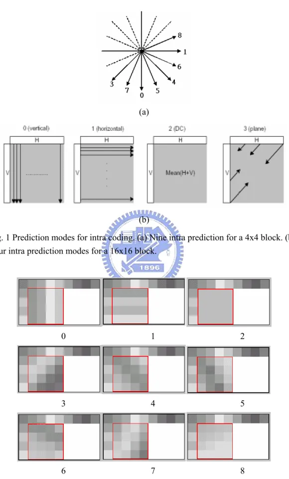
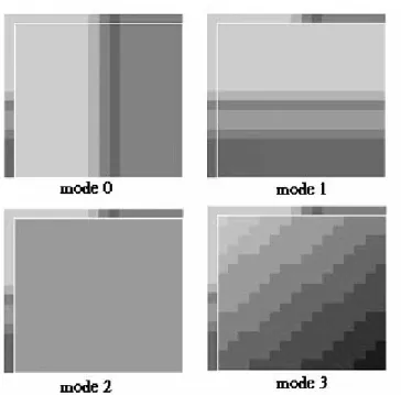
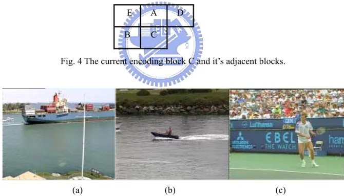
(10) CHAPTER 1 INTRODUCTION Video Coding Experts Group (VCEG-ITU-T SG16 Q.6) launched a project called H.26L in 1998. The goal of the project was to double the coding efficiency compared with previous standards. A new standard named H.264 [1], also named Advanced Video Coding (AVC), was finalized by VCEG and Moving Pictures Expert Group (MPEG-ISO/IEC JTC 1/SC 29/WG 11). H.264/AVC can offer about 50 percent improvement in compression than other previous video coding standard. In order to achieve this goal, some new techniques are used, such as 1/4 pixels resolution of Motion Estimation (ME), variable block size of ME, Integer Discrete Cosine Transformation (Int-DCT), Long-term Memory reference, directional intra mode selection, rate distortion optimization (RDO) technique, in-the-loop deblocking filter, and so on. Although these components can provide efficient compression and high quality, lots of computational time has paid. As shown in Fig. 1, for a 4x4 intra block encoding, H.264 provides nine directional spatial prediction modes to estimate the original 4x4 block, and for a 16x16 intra block encoding, only four directional spatial prediction modes are given to approximate the texture of the 16x16 macroblock (MB). For a 16x16 MB with complicated texture pattern, only dividing it into 4x4 blocks and using more directional spatial prediction modes can get better prediction result. However, for a MB with smooth texture pattern, we could get the good prediction by directly predicting it using less directional spatial prediction modes. In the reference software Joint Model (JM) 8.4 [2] provided by Joint Video Team (JVT), all available modes will be considered, and their corresponding predicted samples can be evaluated via some given equations, Fig. 2 shows the corresponding 1.

(11) predicted samples of each mode for a 4x4 block, which are calculated by the adjacent reconstructed pixels of the 4x4 block, and Fig. 3 shows the same thing but the four predicted samples are a 16x16 block. These predicted samples will be calculated with the original block to get their corresponding prediction errors, and the mode that has the smallest prediction error will be considered as the best mode. The encoder computes the prediction error using rate distortion optimization (RDO) [3]. The RDO cost is given by. J ( s, c, m | QP, λm ) = SSD( s, c, m | QP) + λ m ⋅ R( s, c, m | QP) , where the parameter s denotes the original 4x4 (16x16) luminance block, and c denotes the reconstructed 4x4 block. Parameter m is the available intra mode, QP is the quantization parameter, and the last one λ m is Lagrangian multiplier. The function of J(.) is the Lagrangian function which is calculated by the function SSD(.), sum of square difference between the parameters s and c, and R(.), the number of the coding bits. In the original JM software, the exhaustive search is used to get the best mode. It takes a lot of time. In order to speed up the encoding time, some efforts have been made in intra prediction. Pan et al. [4,5] proposed a directional field based intra mode decision algorithm. The algorithm first applies the Sobel operation to find the edge direction occupied in a block. According to this edge direction, some modes are considered as candidates, and the other modes are discarded. This means that they only search on those candidate modes, so the encoding time are decreased. Although speeding up the time, they still spend much time in deciding candidate modes. Their time saving is about 25%, the average decrement in PSNR is about 0.08dB, and the average increment in bit rate is about 1.76% under certain encoding conditions. 2.

(12) (a). (b) Fig. 1 Prediction modes for intra coding. (a) Nine intra prediction for a 4x4 block. (b) Four intra prediction modes for a 16x16 block.. 0. 1. 2. 3. 4. 5. 6. 7. 8. Fig. 2 Nine predicted samples for a 4x4 block.. 3.

(13) Fig. 3 Four predicted samples for a 16x16 block.. Bojun Meng et. al. [6] also provided an algorithm to speed up intra mode decision. The concepts of their algorithm are described as follows. The mode of the current encoded block has a close correlation to the modes of its adjacent blocks, and this information provides the initial prediction for their algorithm. This initial prediction is called most probable mode (MPM) prediction, and is also used in our proposed algorithm. The other idea of their algorithm is that a mode with direction close to the direction of the best prediction mode is usually a good mode. This concept, which is combined with the downsample prediction, is utilized for the 4x4 intra prediction. For 16x16 intra prediction, they use a condition to detect whether to do 16x16 intra prediction or not, and use the modes of 16 4x4 blocks to predict the 16x16 intra mode. In terms of complexity, they roughly estimate it by the number of pixels that their algorithm need to check, and computational reduction is about 25% 92%. Although the significant reduction of computational time, the computation of predicted samples are not counted in their analysis. 4.

(14) In this thesis, we will propose an efficient algorithm that just takes few amounts of computational operations. First, we will apply the MPM prediction [6] to get the initial guess. Then, based on being predicted samples’ spatial characteristics, a method called Fast Inra-mode Filtering Method (FIFM) is presented to quickly find out the candidate modes, and the final predicted mode for 4x4 intra prediction is then decided. After doing 4x4 intra prediction and before doing 16x16 intra prediction, we investigate a new condition to decide whether to do the 16x16 intra prediction or not. Experimental result shows that our proposed algorithm has gain about 28.288% of time saving with lossless quality and a mere bit-rate increase compared with the standard software under certain encoding conditions. Our algorithm is also superior in time saving, peak signal to noise ration (PSNR), and bit rate to the algorithm proposed by Pan et. al. The rest of the paper is organized as follows. Chapter 2 will describe our proposed algorithm. Chapter 3 gives the experimental results to show the improvement of our algorithm. And the conclusion will be made in Chapter 4.. 5.

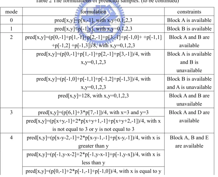
(15) CHAPTER 2 PROPOSED METHOD Intra prediction in JM software can be organized as three parts, 4x4 intra prediction, 16x16 intra prediction, and intra block type decision. For a MB, 16 4x4 blocks will be predicted first that using 4x4 intra prediction, then 16x16 intra prediction is adopted for this MB. Finally, the block type will be decided according to the prediction error. In our proposed algorithm, for a MB, a new 4x4 intra prediction method which will be presented in Sections 2.1 and 2.2, will be adopted first, and then we use the 4x4 intra block type prediction result to decide if it is worth to do 16x16 intra prediction, this part will be described in Section 2.3. If we have decided to do 16x16 intra prediction, 16x16 intra prediction will be conducted, and finally intra block type decision will be adopted as in the JM intra prediction scheme. Section 2.4 will summarize our method and gives a totally encoding scheme of intra prediction.. 2.1 Most Probable Mode (MPM) For an image, adjacent blocks usually have the same edge direction. The reason is that an object usually has similar texture in its interior part. Let C be the block being encoded, A, B, D and E be the adjacent blocks, see Fig. 4. Note that when encoding block C, prediction modes of blocks A and B have been known. By the previous discussion, we know that the prediction mode of block C will be the same as the prediction mode of block A or B with high probability. The JM software uses the modes of block A and B to generate the most probable mode of block C, MPM(C), as follows:. MPM (C ) = Min{IPM ( A), IPM ( B )} , where IPM(A) and IPM(B) represent the intra prediction modes of the reconstructed 6.

(16) blocks A and B respectively. That is, it takes the mode with smaller mode index as the MPM of block C. Here is our experimental analysis shown in Table 1. We take 3 video sequences “Container”, “Coastguard” and “Stefan” files, see Fig. 5, as our test bank. Each test sequence contains 300 frames, and the quantization parameter (QP) is 5, 16, 31 and 48. We compare the MPM with JM 8.4 RDO full search algorithm. We sort the prediction errors of all modes that were calculated by the RDO full search scheme for finding the best intra-coding mode of block C, and if the prediction error of using MPM as the intra-coding mode of block C is the ith smallest in the sorted list, then the block C has an order i. Each block has an order, and the percentage of each order in the whole video sequence will be counted and list in Table 1.. E. A. B. C. D. Fig. 4 The current encoding block C and it’s adjacent blocks.. (a). (b). (c). Fig. 5 The video sequences. (a) container.cif. (b) coastguard.cif. (c)stefan.cif.. 7.

(17) Table 1 The percentage of the orders of most probable mode in RDO full search with QP = 5, 16, 31 and 48. (a) denotes the Container.cif sequence; (b) denotes the Coastguard.cif sequence and (c) denotes the Stefan.cif sequence. QP order. 5. 16. 31. 48. 1. (a) (b) (c) (a) (b) (c) (a) (b) (c) (a) (b) (c) 39.85 44.29 38.87 47.85 46.74 45.95 78.07 62.62 56.18 93.93 95.97 88.44. 2. 15.20 14.20 13.03 15.07 14.32 11.64. 6.95 12.38. 9.15. 2.77. 2.10. 5.22. 3. 10.95. 4. 9.73 10.20. 9.70. 9.49. 9.10. 4.54. 7.47. 8.13. 1.89. 1.13. 3.46. 7.74. 6.97. 7.35. 6.37. 6.64. 6.38. 2.60. 4.39. 5.42. 0.58. 0.35. 1.11. 5. 6.38. 5.85. 6.61. 5.14. 5.44. 5.80. 1.90. 3.46. 4.76. 0.27. 0.18. 0.62. 6. 5.36. 5.09. 6.05. 4.29. 4.74. 5.26. 1.62. 2.88. 4.21. 0.20. 0.11. 0.43. 7. 5.12. 4.81. 6.24. 4.15. 4.47. 5.52. 1.57. 2.60. 4.44. 0.14. 0.08. 0.36. 8. 5.19. 4.87. 6.26. 4.25. 4.51. 5.56. 1.68. 2.64. 4.37. 0.15. 0.08. 0.30. 9. 4.20. 4.20. 5.41. 3.17. 3.65. 4.79. 1.07. 1.56. 3.35. 0.07. 0.02. 0.07. From Table 1, we can see that the MPM has a higher hit rate while the QP value is increasing. This is due to that larger QP value will make MB texture smoother, and the detail in the MB will be removed, this make neighboring MBs have similar content. MPM prediction supports the basic hit rate without costing any computational operations. Therefore, we will use the MPM for the first prediction in our proposed 4x4 intra prediction.. 2.2 Fast Intra-mode Filtering Method (FIFM) Now, we will focus on predicted samples in 4x4 intra prediction. Each predicted sample is calculated by the interpolation according to the direction of the mode. Fig. 6 shows the pixel index of a 4x4 block, where x and y represent the horizontal and vertical coordinate respectively.. 8.

(18) 0. 1 2. 3. x. 0 1 2 3. y Fig. 6 The pixel index of a 4x4 block.. The predicted samples are calculated as shown in Table 2 [1], where p[x,y] represents the reconstructed pixel gray value of coordinate (x,y), pred[x,y] represents the predicted gray value of pixel (x,y), and “>>” denotes the binary shift operation.. Table 2 The formulations of predicted samples. (to be continued) mode. formulation. constraints. 0. pred[x,y]=p[x,-1], with x,y=0,1,2,3. Block A is available. 1. pred[x,y]=p[-1,y], with x,y=0,1,2,3. Block B is available. 2. pred[x,y]=(p[0,-1]+p[1,-1]+p[2,-1]+p[3,-1]+p[-1,0]+ +p[-1,1] +p[-1,2] +p[-1,3])/8, with x,y=0,1,2,3. Block A and B are available. pred[x,y]=(p[0,-1]+p[1,-1]+p[2,-1]+p[3,-1])/4, with x,y=0,1,2,3. Block A is available and B is unavailable. pred[x,y]=(p[-1,0]+p[-1,1]+p[-1,2]+p[-1,3])/4, with x,y=0,1,2,3. Block B is available and A is unavailable. pred[x,y]=128, with x,y=0,1,2,3. Block A and B are unavailable. pred[x,y]=(p[6,1]+3*p[7,-1])/4, with x=3 and y=3. Block A and D are available. 3. pred[x,y]=(p[x+y,-1]+2*p[x+y+1,-1]+p[x+y+2,-1])/4, with x is not equal to 3 or y is not equal to 3 4. pred[x,y]=(p[x-y-2,-1]+2*p[x-y-1,-1]+p[x-y,-1])/4, with x is greater than y. Block A, B and E are available. pred[x,y]=(p[-1,y-x-2]+2*p[-1,y-x-1]+p[-1,y-x])/4, with x is less than y pred[x,y]=(p[0,-1]+2*p[-1,-1]+p[-1,0])/4, with x is equal to y 9.

(19) Table 3 The formulations of predicted samples. 5. Let zVR be set equal to 2*x-y. pred[x,y]=(p[x-(y>>1)-1,-1]+p[x-(y>>1),-1])/2, with zVR equal to 0,2,4, or 6. Block A, B and E are available. pred[x,y]=(p[x-(y>>1)-2,-1]+2*p[x-(y>>1)-1,-1] +p[x-(y>>1),-1])/4, with zVR equal to 1,3, or 5 pred[x,y]=(p[-1,0]+2*p[-1,-1]+p[0,-1])/4, with zVR equal to -1 pred[x,y]=(p[-1,y-1]+2*p[-1,y-2]+p[-1,y-3])/4, with zVR equal to -2 or -3. 6. Let zHD be set equal to 2*y-x. pred[x,y]=(p[-1,y-(x>>1)-1]+p[-1,y-(x>>1)])/2, with zHD equal to 0,2,4, or 6. Block A, B and E are available. pred[x,y]=(p[-1,y-(x>>1)-2]+2*p[-1,y-(x>>1)-1] +p[-1,y-(x>>1)])/4, with zHD equal to 1,3, or 5 pred[x,y]=(p[-1,0]+2*p[-1,-1]+p[0,-1])/4, with zHD equal to -1 pred[x,y]=(p[x-1,-1]+2*p[x-2,-1]+p[x-3,-1])/4, with zVR equal to -2 or -3. 7. pred[x,y]=(p[x+(y>>1),-1]+p[x+(y>>1)+1,-1])/2, with y is equal to 0 or 2. Block A and D are available. pred[x,y]=(p[x+(y>>1),-1]+2*p[x+(y>>1)+1,-1]+ p[x+(y>>1)+2,-1])/4, with y is equal to 1 or 3 8. Let zHU be set equal to x+2*y. pred[x,y]=(p[-1,y+(x>>1)]+p[-1,y+(x>>1)+1])/2, Block B is available with zHU is equal to 0,2, or 4 pred[x,y]=(p[-1,y+(x>>1)]+2*p[-1,y+(x>>1)+1] +p[-1,y+(x>>1)+2])/4, with zHU is equal to 1 or 3 pred[x,y]=(p[-1,2]+3*p[-1,3])/4, with zHU is equal to 5 pred[x,y]=p[-1,3], with zHU is greater than 5. From Fig. 2 and Table 2, we can see that the pixels in the predicted samples have the same intensity along the mode’s direction. For example, Fig. 7 shows the pixel index of block C. For mode 3, those pixels with the same predicted value are grouped together, there are five groups: (b,e), (c,f,i), (d,g,j,m), (h,k,n), and (l,o). If most edge points in the original block C has the same direction as that of a certain 10.

(20) modei, then modei will provide the best predicted samples and be considered as the best mode. On the other hand, if the pixels are quite different in the intensity along the direction of modei, then modei will have little chance to be the best intra predicted mode. To implement the above idea, we use six subtraction operations to calculate the directional difference for each mode, see Table 3. Since mode 2 is DC mode, it has no directional information, we can not get a directional difference. Thus, here we ignore this case. a. b. c. d. e. f. g. h. i. j. k. l. m. n. o. p. Fig. 7 The pixel index of the current encoding 4x4 block.. Table 4 The difference pairs of all the nine modes. mode. calculated pair. 0. (a,e),(a,i), (a,m), (c,g), (c,k), (c,o). 1. (a,b), (a,c), (a,d), (i,j), (i,k), (i,l). 2. x. 3. (b,e), (c,f), (c,i), (d,g), (d,j), (d,m). 4. (c,h), (b,g), (b.l), (a,f), (a,k),(a,p). 5. (a,j),(e,n),(b,k),(f,o),(c.l),(g,p). 6. (a,g),(b,h),(e,k),(f,l),(i,o),(j,p). 7. (b,i),(f,m),(c,j),(g,n),(d,k),(g,i). 8. (c,e),(d,f),(g,i),(h,j),(k,m),(l,n). In each mode, we select six pixel pairs. And the directional difference corresponding to mode m is defined as DD(m),. DD (m ) =. ∑ g (α ) − g ( β ) ,. (α , β ). 11.

(21) where (α,β) is the selected pair in mode m (see Table 3), and g(α) and g(β) are the corresponding pixel values in the original block C. We maintain the three modes that have the smallest directional difference and DC mode, and these four modes are considered as candidate modes. In order to save computing time, for each candidate mode m, we will use the downsampling concept to estimate its prediction error and the estimated prediction error is defined as follows:. DS (m) =. ∑ g (α ) − f. α∈H '. where. m. (α ) ,. H ' = {a, c, f , h, i, k , n, p} is the down sampled set, g(α) is the pixel value in the. original block C, and fm(α) is the predicted sample value using mode m. After all DS(m)s are evaluated, the mode m’ with the smallest DS(m’) is considered as the final mode, and this mode will be the result of FIFM. Note that, in this algorithm, only the candidate modes need to be calculated.. 2.3 Intra Block Type Prediction In JM software, intra block type decision that is made after 4x4 intra prediction and 16x16 intra prediction is inefficient. If we can know that a MB should be encoded in 4x4 intra block type in JM8.4 RDO search scheme, then it is not necessary to do 16x16 intra prediction. Therefore, developing a method to determine if a MB uses 4x4 or 16x16 intra block type coding in advance can help reduce computing time. For a MB using 16x16 intra prediction, we find that its 16 4x4 blocks usually have similar edge directions or the MB tends to be a smooth area. Table 4 shows the simulation results of applying JM8.4 software on some videos. For the QP value equal to 22, the percentages of using 16x16 intra prediction in sequences “container” and “stefan” are both larger than. 12.

(22) “coastguard”. This is caused by the smooth area of the sea surface in “container” sequence and the smooth area of the ground in ”stefan”, while the sea surface contains the detail waves in “coastguard” sequence. Another observation is that the percentage increases abruptly in sequence “coastguard” while the QP value is 22 to 40. This is due to that larger QP makes the detail waves be removed, so the sea surface in “coastguard” becomes smoother. By these observations, for smooth area, the 16x16 intra block type has a high probability to the best mode.. Table 5 The percentage of using 16x16 intra prediction with different QP sequence. container. coastguard. stefan. 10. 6.07%. 0.08%. 6.41%. 16. 15.84%. 0.46%. 14.18%. 22. 29.50%. 1.87%. 17.30%. 28. 50.88%. 10.73%. 20.69%. 34. 59.37%. 38.10%. 27.02%. 40. 68.07%. 67.72%. 39.39%. 46. 86.09%. 89.98%. 79.80%. QP. After doing 4x4 intra prediction, the best prediction mode for each 4x4 block in a MB is decided. According to the above discussion, if there is a dominant mode in the MB (i.e. most of the 16 4x4 blocks in the MB have the same best prediction mode), then the MB may use the 16x16 intra prediction. In the practical implementation, if there is a mode used by most 4x4 blocks and appearing more than Tnum times which is a predetermined threshold, we will consider the mode as a dominate mode in the MB. Here, we give the first constraint for the intra block type decision.. Constraint (1)： Max m. Number (m) > Tnum ,. 13.

(23) where m denotes the intra mode from 0 to 8, and Number(m) represents the number of 4x4 blocks using mode m as the best prediction mode. We now take a look at the prediction error of a 4x4 block. The prediction error for block C using mode m is defined as,. PE (C , m) = ∑ g (C , α ) − f m (C , α ) , α ∈C. where g(C, α) represents the gray value of pixel α in the original block C, and fm(C, α) represents the gray value of pixel α in the corresponding predicted sample of block C using mode m. Obviously, PE(C,m) stands for the sum of the absolute difference (SAD) between block C and its predicted sample using mode m. If a 4x4 block has a large intra prediction error, it means that we can not find a mode to predict this block well. On the other hand, for the 16 prediction errors of the 4x4 blocks in MB, if the variance of these 16 prediction errors is large, then it may have some blocks with a larger errors. This means that some blocks can not be predicted well using 4x4 intra modes, thus the MB has less chance to use 16x16 intra block type coding. By now, we will give the second constraint for the intra block type decision.. 16. Constraint (2)：. ∑ PE (c , m ) − PE * ≤ T i =1. i. i. var. ,. Tvar is a present threshold, ci is the block that has the block index i, mi is the intra prediction mode that has been decided by the 4x4 intra prediction, and PE* is the mean of PE(ci,mi), with i from 1 to 16. We use absolute summation to replace the square summation in the original definition of variance in order to reduce the computation time. For a certain case, only a few blocks have large prediction errors, and others have small prediction errors. For such a MB, if our decision criterion is that if there is a certain block 14.

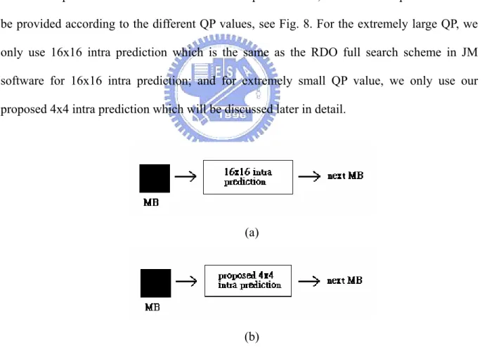
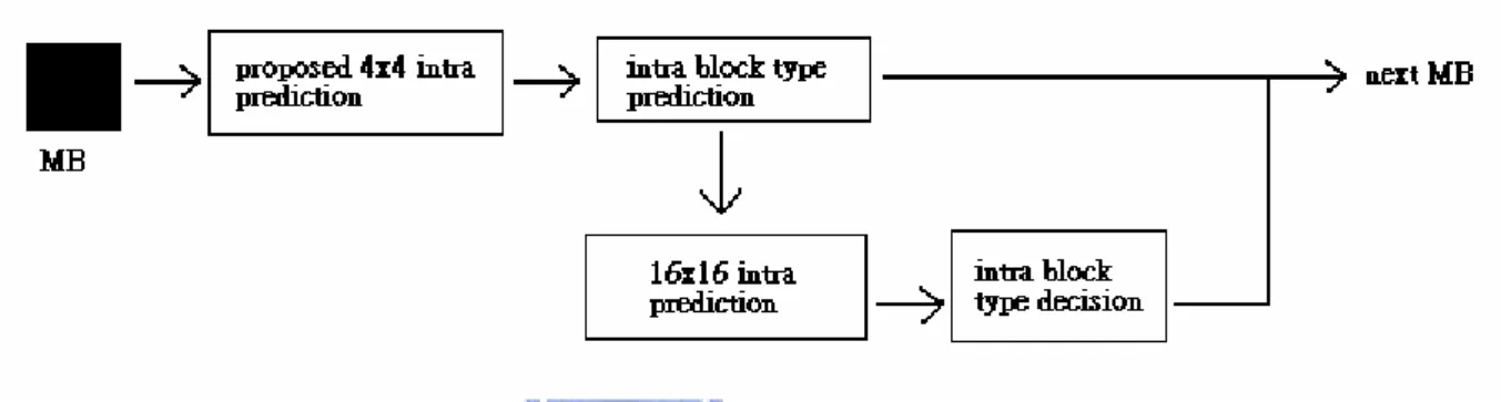
(24) with prediction error lager than a threshold T, then consider the MB is considered to use 4x4 intra prediction. However, the MB still has a chance to use 16x16 intra prediction in the RDO search scheme. This is the reason we use variance of all the prediction errors. In summary, the 16x16 intra block type will be considered as a candidate mode for a MB, if the MB satisfies constraints (1) and (2).. 2.4 Intra Encoding Procedure From Table 3, we have seen that different QP values cause the different percentage of using 16x16 intra prediction. Larger QP causes MB smoother thus, the percentage of using 16x16 intra prediction will increase. To treat this phenomenon, three different procedures will be provided according to the different QP values, see Fig. 8. For the extremely large QP, we only use 16x16 intra prediction which is the same as the RDO full search scheme in JM software for 16x16 intra prediction; and for extremely small QP value, we only use our proposed 4x4 intra prediction which will be discussed later in detail.. (a). (b) Fig. 8 The procedure of intra prediction algorithm for the extreme QP value. (a) QP value is extremely large; (b) QP is extremely small. If the QP value is neither extremely large nor extremely small, we will use the proposed method. The block diagram of the proposed method is shown in Fig. 9. For an MB, our 15.

(25) proposed 4x4 intra prediction is applied first, and, all the 4x4 blocks in this MB will have their intra prediction modes and prediction errors. Next, the intra block type prediction described in Section 2.3 will be adopted to decide whether this MB will use 16x16 intra prediction or not. If the MB does not satisfy constraint (1) or (2) described in Section 2.3, the 4x4 block type coding result will be the final block type mode for this MB, and then next MB will be encoded. Otherwise, we will use the 16x16 intra prediction, which is the same as the RDO full search scheme in JM software for 16x16 intra prediction, then “intra block type decision” will be finally used to decide whether uses 4x4 or 16x16 block type coding according to which block type has the smaller prediction error.. Fig. 9 The block diagram of the intra prediction for the QP value neither extremely large nor small.. The component “proposed 4x4 intra prediction” in Fig. 8(b) and Fig. 9 is shown in Fig. 10. Before describing the flow chart of this component, we introduce two elements first, “Good Enough Test” and “Boundary Test”. “Good Enough Test” is defined as. PE (C , mc ) < PE ( A, IPM ( A)) and PE (C , mc ) < PE ( B, IPM ( B )) , where A, B, and C are the blocks described before. IPM(A) and IPM(B) are the intra prediction modes of reconstructed blocks A and B respectively. mC represents the mode we. 16.

(26) predicted by our prediction method. We will consider the mC is a good mode for block C if the prediction error is smaller than the prediction error of block A and B. And the other element “Boundary Test” is to check if the current encoded block is locating on the top boundary or left boundary in an image. For each 4x4 image block, we will first do “Boundary Test”, if the block locates on the boundary, “Full Prediction” will be adopted which will be given a fine definition later, otherwise we use “MPM Prediction” to get a initial prediction mode. Then the “Good Enough Test” is used to decide whether the MPM is a good mode or not. If the MPM is good enough, IPM(C) will set to MPM, then we check if there still have some blocks do not be encoded in this MB or not. Otherwise, “FIFM Prediction” will be adopted. The mode mfifm predicted by the FIFM will be tested by the “Good Enough Test” too, as the same situation as before, if the mode mfifm is considered as a good mode, IPM(C) will set to mfifm. Otherwise, the final step “Full Prediction” will be used. The mode mfull of “Full Prediction” is defined as follows,. m full = arg min{PE (C , m)} . 0 ≤ m ≤8. After doing “Full Prediction”, IPM(C) will set to mfull, and then check if there still have blocks that do not be encoded.. 17.

(27) Boundary Test. Yes. 4x4 image block No. MPM Prediction. Yes. Good Enough Test. Yes. No Still has block not. FIFM. encoded. Prediction. No. Yes. Good Enough Test No Full. Next Step. Prediction. Fig. 10 The proposed 4x4 intra prediction diagram.. 18.

(28) CHAPTER 3 EXPERIMENTAL RESULTS The proposed algorithm is implemented into H.264 JM8.4 codec. It is compared with the RDO full search scheme in H.264. We also compared the method proposed by Pan et. al. and list the comparison results in Table 5. Sequences used are “Coastguard.qcif”, “Container.qcif”, “Foreman.qcif”, “News.qcif”, “Silent.cif”, “Bus.cif”, “Mobile.cif”, “Paris.cif”, “Stefan.cif” and “Tempete.cif”, and the period of I-frames is set to 100, i.e., there is one I-frame for every 100 coded frames, and the rest are the P-frames. QP values are set to be 28, 32, 36, and 40, which are the same as that in Pan’s paper. “△Bits”, “△Time”, and “△Psnr” denotes the average change of the bit rate, average change of the total encoding time, and average change of the PSNR respectively, comparing to the results of RDO full search scheme. The negative value means less than the compared data, and the positive value means more than the compared data. In Table 5, we can see that our proposed method provides about 28.288% time saving, PSNR loss about 0.0564 dB, and bit rate rising about 0.939%. On the other hand, Pan’s method provides about 25.272% time saving, 0.0637 dB PSNR loss, and 1.427% bit rate rising. These results show that our method is superior to Pan’s. We also plot the RD cost of the “Foreman.qcif” and “Mobile.cif” sequences in Fig. 11. As shown in Fig. 11, our proposed process has a much-closed curve with the original JM8.4 scheme. This means that we could pay few bit-rates and loss a little quality to gain lots of time saving.. 19.

(29) Table 6 The experimental results. Sequence. △Time(%). △Psnr(dB). △Bits(%). Proposed Pan’s. Proposed Pan’s. Proposed Pan’s. Coastguard(qcif). -24.785. -22.594. -0.010. -0.006. 0.405. 0.214. Container(qcif). -27.936. -22.310. -0.080. -0.106. 1.947. 2.439. Foreman(qcif). -23.657. -21.864. -0.040. -0.104. 0.984. 2.190. News(qcif). -28.018. -22.987. -0.108. -0.113. 1.157. 2.143. Silent(qcif). -25.781. -22.697. -0.123. -0.071. 0.774. 1.608. Bus(cif). -29.239. -27.652. -0.015. -0.018. 0.57. 0.431. Mobile(cif). -31.908. -29.266. -0.023. -0.032. 0.699. 0.822. Paris(cif). -32.826. -27.804. -0.065. -0.075. 1.401. 1.643. Stefan(cif). -28.925. -27.401. -0.060. -0.055. 0.821. 1.238. Tempete(cif). -29.807. -28.147. -0.040. -0.057. 0.631. 1.545. average. -28.288. -25.272. -0.056. -0.064. 0.939. 1.427. (a) Fig. 11. The RD curves of the sequences. (a) Foreman_qcif, (b) Mobile_cif. (continued). 20.

(30) (b) Fig. 11. The RD curves of the sequences. (a) Foreman_cif, (b) Mobile_cif.. 21.

(31) CHAPTER 4 CONCLUSION We have proposed an efficient algorithm for H.264 intra encoding process in this paper. The algorithm uses MPM, FIFM and intra block type prediction algorithm to speed up the intra encoding process. Experimental result shows that we can gain about 28.288% time saving for the sequence of intra period 100. It also shows that the loss of PSNR is negligible and the bit rate is similar to that of the original scheme. Comparing to the Pan’s algorithm, our proposed method has better result in time saving, increase of bit rate, and loss of PSNR.. 22.

(32) REFERENCES [1] “Draft ITU-T recommendation and final draft international standard of joint video specification ITU-T Rec. H.264/ISO/IEC 14 496-10 AVC,” in Joint Video Team (JVT) of ISO/IEC MPEG and ITU-T VCEG, JVTG050, 2003. [2] Joint Video Team (JVT), reference software “Joint Module Version 8.4,” http://iphome.hhi.de/suehring/tml/download/old_jm/jm84.zip [3] C. Kim, H. H. Shih, and C. C. Jay Kuo, “Feature-Based Intra-Prediction Mode Decision for H.264,” IEEE International Conference on Image Processing, Vol. 2, pp. 769-772, Oct. 2004. [4] F. Pan, X. Lin, S. Rahardja, K. P. Lim, and Z. G. Li, “A Directional Field Based Fast Intra Mode Decision Algorithm For H.264 Video Coding,” IEEE International Conference on Multimedia and Expo, Vol. 2, pp. 1147-1150, June 2004. [5] F. Pan, X. Lin, et. al., “Fast Mode Decision for Intra Prediction,” ISO/IEC JTC1/SC29/WG11 and ITU-T SG16 Q.6, JVT 7th Meeting, Pattaya ІІ, Thailand, March 2003. [6] B. Meng, O. C. Au, C. W. Wong, and H. K. Lam, “Efficient Intra-Prediction Algorithm in H.264,” IEEE International Conference on Image Processing, Vol. 3, pp. 837-840, Sept. 2003. [7] I. E. G. Richardson, “H.264/MPEG-4 Part 10: Intra Prediction,” http://www.vcodex.com, April 2003.. 23.

(33)