國 立 交 通 大 學
電子工程學系電子研究所
博 士 論 文
大鄰近層細胞非線性網路與比例式記憶細胞非線性
網路之設計與分析
THE DESIGN AND ANALYSIS OF
LARGE-NEIGHBORHOOD CELLULAR
NONLINEAR NETWORKS AND RATIO-MEMORY
CELLULAR NONLINEAR NETWORKS
研 究 生:陳勝豪
指導教授:吳重雨 博士
大鄰近層細胞非線性網路與比例式記憶細胞
非線性網路之設計與分析
THE DESIGN AND ANALYSIS OF
LARGE-NEIGHBORHOOD CELLUNLAR
NONLINEAR NETWORK AND RATIO-MEMORY
CELLULAR NONLINEAR NETWORK
研 究 生:陳勝豪 Student: Sheng-Hao Chen
指導教授:吳 重 雨 博士 Advisor: Dr. Chung-Yu Wu
國立交通大學
電子工程系電子研究所
博士論文
A Dissertation Submitted toDepartment of Electronics Engineering and Institiute of Electronics College of Electrical and Computer Engineering
National Chiao-Tung University In Partial Fulfillment of the Requirements
For the Degree of Doctor of Philosophy
In
Electronics Engineering June 2009
Hsinchu, Taiwan, Republic of China
i
大鄰近層細胞非線性網路與比例式記憶細胞非
線性網路之設計與分析
研究生:陳勝豪 指導教授:吳 重 雨 博士 國立交通大學電子工程系電子研究所摘 要
此論文研究針對於類神經網路(細胞非線性網路)的研究與應用,細胞非線性 網路模仿神經聯結方式運算,可視為一類比式計算機處理單元陣列,適合運用在 影像處理,雖然目前數位式計算機處理單元可以達到數個GHz的處理速度,但在影 像處理方面,若以各個圖元分別作運算,仍需要大量的處理時間,因此若以細胞 非線性網路陣列平行運算,可達到高速運算的結果,並針對神經網路之特性與其 優缺點,以類比電路實現為主軸,分別實現以下兩個部分: 1. 設計分析一可程式化之大鄰近層細胞非線性網路通用機器核心部分。 2. 設計分析一可學習之免衰減比例式記憶細胞非線性網路與一反覆學習比例式 記憶細胞非線性網路。 目前細胞非線性網路通用機器僅能處理3x3的範本,即僅有鄰接的各圖元間有 係數的關聯,而大鄰近層細胞非線性網路的主要構想,在於若可將關聯推性廣至 更遠之細胞上,可增加細胞非線性網路的功能性;此外,亦有其他團隊針對將大 鄰近層細胞非線性網路的範本,分解成數個3x3的範本來達到相同的功能,因此若 能設計一大鄰近層細胞非線性網路,一步完成大鄰近層細胞非線性網路的功能, 可節省所需之處理時間與消耗功率;因為大鄰近層細胞非線性網路為一大型陣 列,電路設計方面主要考慮其功率消耗與面積大小,並以傳導式連結的電路架構, 使其可實現大鄰近層細胞非線性網路的功能,論文中許多大鄰近層細胞非線性網ii 路的範本,皆可在模擬中實現,而 所設計之大鄰近層細胞非線性網路陣列大小為 20 × 20,晶片大小為1543 μm × 1248 μm,功率消耗在待機時僅0.7 mW,一般操作 下為 18 mW,操作頻率為20 MHz,並在實現中驗證可實現人的錯覺範本。 可學習之比例式記憶細胞非線性網路目的在於學習各種樣本,並將含有雜訊 的樣本復原,原理是將兩個圖元間的關係,紀錄在比例式記憶體的電容中,並利 用其漏電的缺點強化圖元間的關係,並將各個圖元周圍的範本常態化(normalized), 因此稱之為比例式記憶,藉此可提高其辨識率;然而,由於各個圖元間的差異, 若以相同的放電時間強化圖元間關係,可能會造成此關係被破壞或是強化不足, 因此各個關係改以與圖元周圍的關係平均來決定其值的去留,以此方式可節省除 法器的運用並簡化比例式記憶細胞非線性網路的複雜度。另外,從機率統計方面 亦可推論出臨界值範本的必要性,即為其臨界值範本(Threshold),由此提出以遞迴 學習的方式,統計出雜訊與辨識後的臨界值,藉此可更加增加其辨識率。 本論文之主要貢獻為,建立一完整大鄰近層細胞非線性網路之架構,並以簡 單之電路實現,因此可達到小面積、低功率,經實驗量測可用於二元(binary)的影 像運算;另外不需放電之可學習之比例式記憶細胞非線性網路方式,亦簡化了電 路的複雜度,使其容易實現。亦討論了可學習比例式記憶細胞非線性網路之機率 統計模型,並依據推論結果,運用臨界值範本的學習,更增進其辨識率。
iii
THE DESIGN AND ANALYSIS OF LARGE-
NEIGHBORHOOD CELLULAR
NONLINEAR NETWORK AND RATIO-
MEMORY CELLULAR NON-LINEAR NETWORK
Student: Sheng-Hao Chen Advisor: Dr. Chung-Yu Wu
Institute of Electronics Engineering National Chiao-Tung University
Abstract
This dissertation focuses on the studies and applications of the cellular neural/nonlinear networks (CNN). CNN is an analog CPU array which can imitate the operations of neural connections which is suitable for image processing. Although the speed of the recent digital CPUs can reach higher than several GHz, when the digital CPU is applied on the image processing, it takes a lot of time to achieve the processing separately. Hence, the advantage of parallel processing of CNN array is required to achieve high speed processing. According to the properties of CNN, two major topics are realized by using analog circuit design.
I. The design and analysis of a CMOS low-power, large-neighborhood CNN with propagating connections
II. The design and analysis of a ratio memory CNN
Recently, cellular nonlinear network universal machine (CNNUM) can only achieve the 3 × 3 templates of nearest connecting correlations. The main concept of large-neighborhood cellular nonlinear network (LNCNN) is to extend the connecting correlations and to increase the capability of CNN. Moreover, some studies have
iv
decomposed the LNCNN templates into several 3 × 3 templates to realize the same functions. However, this may take more cost to achieve one LNCNN function. Hence, it is necessary to design a LNCNN for the templates larger than 3 × 3.
Because LNCNN is a very large scale array, the power consumption and chip area are considered first. With the propagating connections, the functions of LNCNN are realized by the designed 20 × 20 LNCNN array and the chip size is 1543 μm × 1248 μm. The power consumption is 0.7 mW on standby and 18 mW in operation with a system clock frequency of 20 MHz.
The purpose of the learnable ratio memory cellular nonlinear networks is to learn the every kind of patterns and recover the learned noisy patterns. The concept is to store the correlations of two neighboring cells on the capacitor in the ratio memories and use the intrinsic leakage to enhance the common characteristics. Moreover, the templates are normalized by the correlation with neighboring cells to increase the recognition rate and thus, it is called ratio memory. However, due to the difference of any two cells, if the same elapsed time for leakage is applied to enhance the characteristics, it may cause only the self-feedback term to remain or the enhancement of common characteristics to be smaller. Hence, the templates are decided by the correlation and the mean of the four correlations around one cell. This can make the design much easier and the divider can be abandoned. Besides, by the deviation of the statistics and probability, there exists a dc term except for the templates. It is found that the threshold template is required and learned by recursive learning to gather the information of the noisy patterns to increase the recognition rate.
The main contribution of this dissertation is that the complete architecture of large-neighborhood CNN has been established and realized by a simple circuit design. Hence, a small-size, low-power LNCNN chip has been fabricated and measured. According to the experimental result, the LNCNN chip can be applied on the binary image processing. Moreover, the statistic and probability models of the learnable ratio memory CNN has also been derived and, according to the results, the learning of the threshold templates are used to increase the recognition rate. Furthermore, the learnable
v
ratio memory CNN without elapsed time has also been proposed to simplify the complexity of the circuits for realization.
vi
致 謝
首先感謝我的指導教授吳重雨教授,學術上循序漸進地細心指導,適時給予 建議,使我能順利的完成學業,而教授在生活上也時時刻刻關心,了解學生的想 法,因此不僅在研究方面,學習到老師嚴謹的態度,亦於待人處世上獲益良多; 另外也要感謝和藹可親的師母曾昭玲女士,謝謝她常常給予我關懷與打氣加油。 感謝實驗室的學長姐、同學以及學弟妹的協助,使我在這六年來的博士班生 涯更加的豐富,也使得我的研究更加順遂。感謝鄭秋宏、黃冠勳、廖以義、施育 全、賴瑞麟、周忠昀、林俐如、虞繼堯、王文傑及蘇烜毅學長姐的經驗與教導, 不論是知識的啟發或是處事的方法上,皆幫助了我許多;也感謝楊文嘉、黃祖德、 陳煒明、雄霆等同期的同學,一同討論、聊天、發洩,共同做研究、傾洩攻讀博 士班的壓力;另外也感謝學弟妹們,幫忙處理事務以及計畫研究;感謝實驗室助 理卓慧貞小姐(蛤~~~),以及中心助理何淳伶及小小黃瑋屏,在行政事務上的協 助;還有好朋友小邱跟小邱姐姐的鼓勵,常常一起去大潤發瞎拼發洩,我會好好 照顧妳們送的漂亮包包;有了學長姐、同學、學弟妹以及好朋友的幫助鼓勵下, 我的論文才得以順利完成,因此在此也祝福諸位學業上能順利畢業,事業上能一 帆風順。 最後我要致上最深的的感謝,給我的父親陳振源先生與我的母親葉柳青女士, 由於您們的從小的教養以及支持鼓勵,讓我得以最大的力量,來完成博士班的學 業,感謝您們無怨無悔的付出,並且在我心情不好時承受了我的不滿,在此對您 們表示深深的歉意,我愛您們,我的爸媽。 陳 勝 豪 誌於 風城交大 九十八年夏vii
CONTENTS
ABSTRATE (CHINESE) ...i
ABSTRATE (ENGLISH)... iii
ACKNOWLEDGEMENTS...vi
CONTENTS ... vii
TABLE CAPTIONS...ix
FIGURE CAPTIONS ...x
CHAPTER 1 INTRODUCTION...1
1.1 BACKGROUND OF ARTIFICIAL NONLINEAR NETWORKS...1
1.2 RESEARCHESONCNNSANDTHEIRAPPLICATIONS...11
1.3 REVIEWOFLNCNNS ANDRMCNNS...14
1.4 RESEARCHMOTIVATIONANDORGANIZATIONOFTHIS DISSERTATION...17
CHAPTER 2 THE DESIGN AND ANALYSIS OF A CMOS LARGE-NEIGHBORHOOD CNN WITH PROPAGATING CONNECTIONS...21
2.1 INTRODUCTIONS ...21
2.2 ARCHITECTURE AND MODELS ...23
2.3 CIRCUIT IMPLEMENTATION AND SIMULATION RESULTS ...30
2.4 EXPERIMENTAL RESULTS...49
2.5 SUMMARY...54
CHAPTER 3 THE DESIGN AND ANALYSIS OF A CMOS RATIO-MEMORY CNN WITHOUT ELAPSED TIME...56
3.1 INTRODUCTION ...56
3.2 ARCHITECTURE AND MODELS ...58
3.3 CIRCUIT IMPLEMENTATION WITH SIMULATION RESULTS ...65
3.4 EXPERIMENTAL RESULTS...79
viii
CHAPTER 4 THE ANALYSIS OF THE RECURSIVE LEARNING RMCNN...87
4.1 INTRODUCTION ...87
4.2 MATHEMATICAL ...88
4.3 SIMULATIONRESULTS...93
4.4 SUMMARYANDFUTUREWORK ...95
CHAPTER 5 CONCLUSIONS AND FUTURE WORK...98
5.1 CONCLUSIONS...98
5.2 FUTURE WORK...100
ix
TABLE CAPTIONS
Table 2.1 DERIVED EQUATIONS OF TEMPLATE COEFFICIENTS AND GAINSOFSYNAPSES ...29 Table 2.2 COMPARISON OF DEVICE NUMBERS AND
INTERCONNECTIONLINES ...40 Table 2.3 COMPARISON OF LNCNN WITH CNNUC3 [132]-[133] AND
ACE16K[131]...53 Table 2.4 COMPARISONOFTHEPROPOSED LNCNNANDLNCNNWITH
SYMMETRICTEMPLATES...54 Table 3.1 THECOMPARISONSOFTEMPLATESAINCELL(4,5),CELL(5,3),
CELL(8, 5), AND CELL(7, 5) BETWEEN RMCNN WITH AND WITHOUTELAPSEDTIME...74 Table 3.2 THEDESCRIPTIONOFEACHCONTROLSIGNAL ...80 Table 3.3 THE COMPARISON OF THE ABSOLUTE WEIGHTS A44 WITH
MATLABANDHSPICEINDIFFERENTCONDITIONS...84 Table 3.4 COMPARISON BETWEEN RMCNN AND RMCNN REQUIRING
NO ELAPSED TIME ...85 Table 4.1 THEREQUIREDITERATIONSTOFITTHECONSTRANSWHERE
7PATTERNSARELEARNED ...95 Table 4.2 THEREQUIREDITERATIONSTOFITTHECONSTRANSδ=0.03
x
FIGURE CAPTIONS
Fig. 1.1 The simplest computational element or node which forms a weighted
sum of N inputs and passes the result through the nonlinearity...2
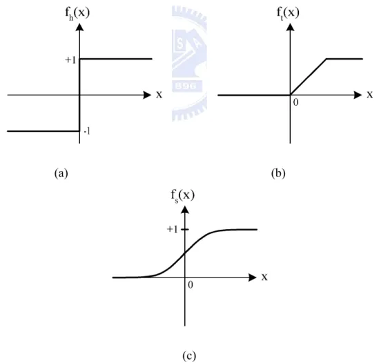
Fig. 1.2 The three common types of nonlinearity of (a) hard limiters, (b) threshold logic elements, and (c) sigmoidal nonlinearities. ...2
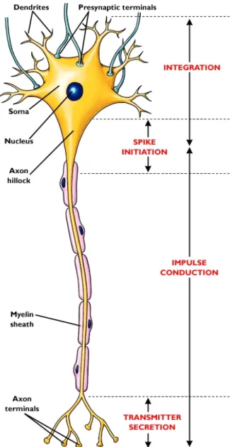
Fig. 1.3 The biological model of a neuron cell which contains the cell body (nucleus) and the I/O terminals of dendrites and axon terminals...4
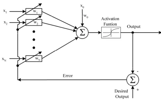
Fig. 1.4 The simplest architecture of an adaptive linear element where its weights are determined by the normalized least mean square training law by a preset desired output. ...6
Fig. 1.5 A perceptron with a sigmoidal activation function. The threshold value w0 are initialized to small non-zero values. ...7
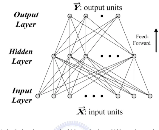
Fig. 1.6 A simple three-layer network which contains input, hidden, and output layers...8
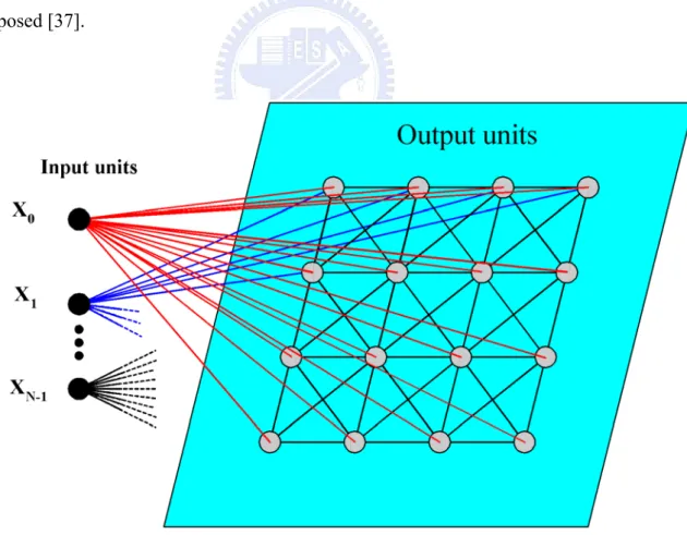
Fig. 1.7 Two-dimensional array of Kohonen’s self-organizing feature maps. ...9
Fig. 1.8 The RC circuit model of a CNN cell. ...10
Fig. 1.9 The core architecture of CNN with templates A and B...11
Fig. 2.1 The architecture of a LNCNN kernel unit...24
Fig. 2.2 The structure of the BODY in Fig. 2.1...25
Fig. 2.3 The large-neighborhood template generated by a LNCNN with propagating connections...28
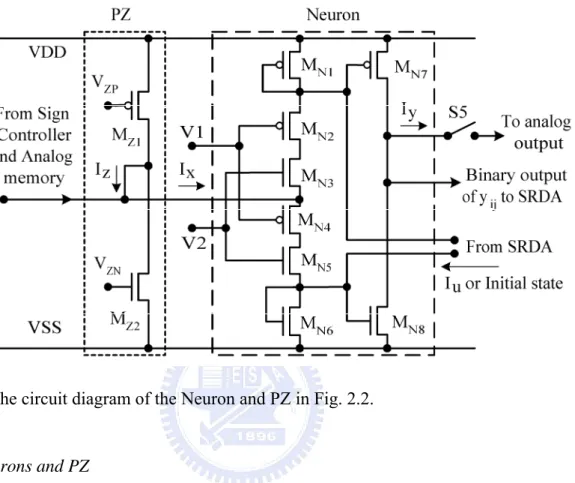
Fig. 2.4 The circuit diagram of the Neuron and PZ in Fig. 2.2. ...31
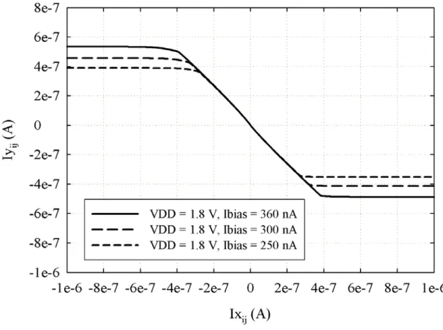
Fig. 2.5 The transfer characteristic of a neuron with different external bias currents Ibias. ...32
Fig. 2.6 The circuit diagrams of (a) the synapses PL2, PR2, PD2, and PU2; (b) the synapses PL1, PR1, PD1, and PU1; (c) the synapses PRU, PRD, PLU, PLD, and PS; (d) the Sign Controller. ...35
xi
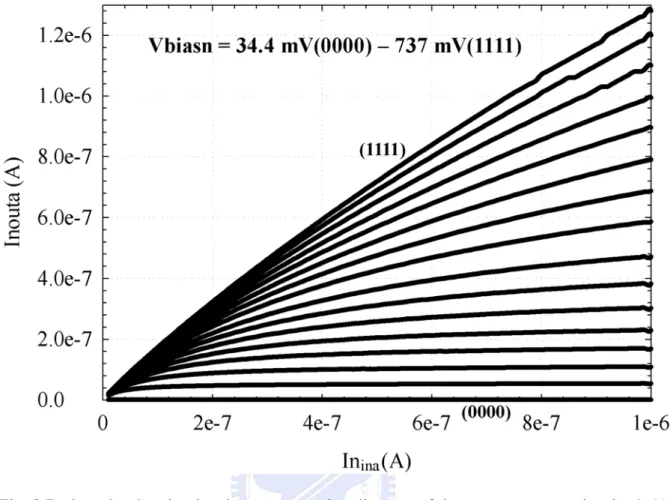
Fig. 2.7 The HSPICE simulated Inouta vs. Inina diagram of the N-type synapse
in Fig. 2.6(a) with 16 different values for Vbiasn. ...36
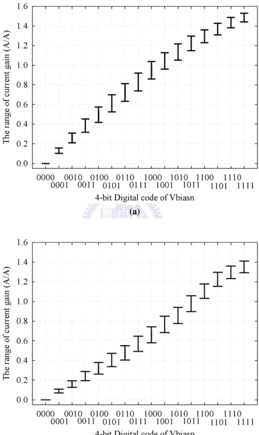
Fig. 2.8 The range of (a) the N-type current gains and (b) the P-type current gain of the synapses with an input current range from 300 nA to 500 nA...37
Fig. 2.9 The circuit diagram of the PSW. ...39
Fig. 2.10 The circuit diagram of the analog memory. ...41
Fig. 2.11 The architecture of the 20x20 LNCNN system...42
Fig. 2.12 The timing diagram of the controlled signals in LNCNN...43
Fig. 2.13 The 5 x 5 templates B, A and Z for Muller-Lyer illusion [40]...44
Fig. 2.14 The extracted values of the diamond-shaped template from a HSPICE post-layout simulation. ...45
Fig. 2.15 (a) The input patterns of Muller-Lyer illusion. (b) The resultant output pattern of Muller-Lyer illusion from the HSPICE simulation result...45
Fig. 2.16 The template B of 5x5 and diamond-shaped templates of (a) diffusion [138] and (b) de-blurring [40]. ...47
Fig. 2.17 The input patterns and simulation results of (a) diffusion and (b) de-blurring. ...48
Fig. 2.18 The input and output patterns of erosion with 3 × 3 neighborhood templates [40] in two iterations and with diamond-shaped templates in one iteration. ...49
Fig. 2.19 A photograph of the fabricated 20 × 20 LNCNN chip...50
Fig. 2.20 The experimental resultant output pattern of Muller-Lyer illusion...51
Fig. 2.21 The experimental results of Pixel B with the signal Operation_Start. ...52
Fig. 3.1 The general architecture of the RMCNN. ...62
Fig. 3.2 (a) The input stage and neuron, (b) RM, and (c) comparator and counter in the kernel unit of RMCNN...63
Fig. 3.3 (a) The circuits of the blocks VTI1 and Neuron. (b) The transfer characteristic of the block VTI1. ...66
Fig. 3.4 (a) The circuit of the blocks VTI2 (with ME) and VTI3 (without ME) (b) The transfer characteristic of the block VTI2 and VTI3. ...68
xii
Fig. 3.5 The circuit of the block W...69
Fig. 3.6 The block diagram of the sign controller where the detector is composed of two cascaded inverters. ...69
Fig. 3.7 The circuit of the block COMP. ...69
Fig. 3.8 The four absolute currents from VTI3 are averaged and compared with the mean current. ...71
Fig. 3.9 Input patterns in the learning period...72
Fig. 3.11 The recognition rates by using proposed RMCNN and by being directly amplified...73
Fig. 3.12 The comparison of the recognition rates by using proposed RMCNN with self-feedback, without self-feedback of 50% tolerance and by being directly amplified...74
Fig. 3.13 The comparison of recognition rates with 3 × 3 neighborhood templates and large neighborhood diamond templates of r’=3...75
Fig. 3.14 The ratio weights of RMCNN with different elapsed time. ...76
Fig. 3.15 The recognition rates of (a) 3 × 3 neighborhood and large neighborhood templates by repeating the operation of the proposed algorithm (marked with ‘modified’) where 7 patterns are learned. ...78
Fig. 3.16 The modified circuits of block COMP that can realize the repeated proposed algorithm...78
Fig. 3.17 The architecture of a 9x9 RMCNN without elapsed time chip. ...79
Fig. 3.18 The timing diagram of control signals...81
Fig. 3.19 The photograph of the RMCNN without elapsed time chip...81
Fig. 3.20 The uniform noisy patterns for measurement...82
Fig. 3.21 Experimental results of recognized patterns in the recognition period after a set of patterns with noise level 0.25 are recognized...82
Fig. 3.22 Experimental output waveform of the third recognized pattern...83
Fig. 3.23 The modified circuit of the block W. ...85
xiii
Fig. 4.2 The probability density of the input uC2...90 Fig. 4.3 The probability density of the state xC1 after recognition...90 Fig. 4.4 The error rates produced by the shadow part when the output of the pixel
C1 should be (a) 1 and (b) -1...92 Fig. 4.5 The procedure of the recursive learning algorithm. ...92 Fig. 4.6 The recursive learning of THR(i,j) in nth iteration...92 Fig. 4.7 The recognition rates of RMCNN requiring no elapsed time without and
with recursive learning of constrains 0.01, 0.03, and 0.05 where 7 patterns are learned...94 Fig. 4.9 The recognition rates where 6 patterns and 8 patterns are learned with
C H A P T E R 1
INTRODUCTION
1.1 BACKGROUND OF ARTIFICIAL NONLINEAR
NETWORKS
Brain, one of the world’s best computers, makes human devoted to investigating it to expose the source of powerful functions. With the analog neuron models, the artificial neural networks (ANNs) proposed by Hopfield [1]-[5] and Chua et al. [6]-[8] have firstly been implemented in circuitry [10]. Since then, ANNs have attracted strong interest of researchers to explore their scientific and engineering applications. The models of ANNs [9], [5], [11] which are based on the understanding of biological nervous systems, attempt to achieve good performance by the dense interconnection of simple computational elements. Computational elements or nodes are connected via weights that are typically adapted during the operation such as Hopfield net [1]-[10], [11], Hamming net [11]-[15], et al. The simplest node sums N weighted inputs and passes the result through the nonlinear function f(•) as shown in Fig. 1.1 [11], [16]. In Fig. 1.1, the output y can be illustrated as
⎟ ⎠ ⎞ ⎜ ⎝ ⎛ − =
∑
− = 1 0 N i i ix w f y θ (1.1).Fig. 1.1 The simplest computational element or node which forms a weighted sum of N inputs
and passes the result through the nonlinearity.
(a) (b)
(c)
Fig. 1.2 The three common types of nonlinearity of (a) hard limiters, (b) threshold logic
where xi is the ith input, wi is the ith weight factor, and θ is the internal threshold. The node is
characterized by an internal threshold or offset θ and by the type of the nonlinearities. Fig. 1.2(a)-(c) illustrate three common types of nonlinearity: hard limiters (threshold functions), piecewise linear functions, and sigmoidal nonlinearities. The common characteristic of these three nonlinearities is that the output y is saturated at both ends. More complex nodes may include temporal integration or other types of time dependencies and more complex mathematical operations than summation.
For comparison, silicon devices have an intrinsic speed about 100,000 times faster than that of natural neurobiological devices. However, in solving problems like face recognition, the neurobiological system is more effective by a factor of 108 [17]. In the biological model of a neuron cell as shown in Fig. 1.3, the neuron contains cell body (nucleus) and the synapses, which are the I/O terminals of the neuron and can be classified as dendrites and axon terminals by their essential functions, are illustrated. Dendrites can receive excitation or inhibition signals from other neurons or external environment. Axon terminals can pass the excitation or inhibition signals to next neurons. Through different functions, different intensities of the excitation or inhibition signals can be transferred to next neurons. The second neuron next to the first one receives the signals from the axon terminals of the first neuron and other neurons, makes a decision by the sigmoidal nonlinearity, and sends another excitation or inhibition signals to next neurons through axon terminals. By using the similar this architecture that a brain-style computational device is richly connected to one another, an artificial neural or nonlinear network is constructed. The function it computes is determined by the pattern of connections. Based on the models of ANNs, many new topologies and algorithms are developed.
Fig. 1.3 The biological model of a neuron cell which contains the cell body (nucleus) and the
I/O terminals of dendrites and axon terminals.
Work on the models of ANNs has a long history. Development of detailed mathematical models has begun about 60 years ago in the work of McCullock and Pitts [18], Hebb [19], Rosenblatt [20], Widrow [21], et al. In 1980s, the work by Hopfield [1]-[10], Rumelhart and McClelland [22], Sejnowski [23], Feldman [9], Grossberg [24]-[25], et al. has led to a new resurgence of the field. There seems to be five reasons for the rebirth. First, the faster and faster computer makes it possible to simulate and experiment with much larger and more
interesting networks than that in 1950s and 1960s. Second, it is believed that the faster computers must be in parallel computation. However, it is generally easier to build parallel computers than to find algorithms that are efficient. Third, the empirical tools of neuroscience are expanding and more and more knowledge about how the neuron functions is learned. Besides, it is hoped that the theoretical tools developed in the study of neural network computational systems will allow for the modeling of the real neural networks. Fourth, theoretically, Hopfield provides the mathematical foundation for understanding the dynamics of the recurrent networks. The mathematical model has been extended and applied by Hinton and Seinowski [26], Cohen and Grossberg [27], Smolensky [28] and a number of scientists to provide more mathematical models and solve important problems such as optimization. Fifth, with the extension of Rosenblatt, Widrow, and Hoff’s work dealing with learning in a complex, multi-layer network [20]-[21], this provided a technique, known as the back-propagation learning algorithm [29], is developed that multilayer perceptron-like devices can be reliably trained.
The interest in ANNs comes from the networks’ ability to mimic human brain as well as its ability to learn and respond. Adaptation or learning is a major focus of ANN research that provides a degree of robustness to the ANN model. An adaptive linear element is a single neuron of McCulloch-Pitts type, where its weights are determined by the normalized least mean square (LMS) training law. The LMS learning algorithm was originally proposed by Widrow and Hoff [21]. This learning rule is also referred to as the delta rule. It is a well-established supervised training method that has been used over a wide range of diverse applications [30]-[33]. The simplest architecture of an adaptive linear element is shown in Fig. 1.4. In the simplest adaptive linear element, the neuron with a linear activation function is used. The weights are adjusted by the LMS error of comparing the output with the desired output.
Fig. 1.4 The simplest architecture of an adaptive linear element where its weights are
determined by the normalized least mean square training law by a preset desired output.
Once the weights are properly adjusted, the response of the trained unit can be tested by applying various inputs which are not in the training set. If the network produces consistent responses to a high degree with the test inputs, it is said that the network can generalize. Therefore, the process of training and generalization are two important attributes of the network. Similar to the adaptive linear element, the original idea of the perceptron has been develop by Rosenblatt in the late 1950s along with a convergence procedure to adjust the weights [20]. The original perceptron convergence procedure is developed by Minsky and Papert [34] as shown in Fig. 1.5. The perceptron [20] by Rosenblatt is based on the McCulloch-Pitts model of the neuron with the hard limitation activation function where the inputs are binary and no bias is included. The perceptron of Minsky and Papert is similar to that by by Rosenblatt except for the addition of an activation function and the non-zero value of the threshold w0 [34].
Fig. 1.5 A perceptron with a sigmoidal activation function. The threshold value w0 are
initialized to small non-zero values.
The perceptron convergence procedure and its variants are limited to simple one-layer networks involving only input and output units. It maps similar input patterns to similar output patterns. The similarity of patterns in the system is determined by their overlap which is decided outside the learning system by whatever produces the patterns. Therefore, the constraint of the system leads to an inability to learn certain mappings from input to output. In a multilayer network, the information coming to the input units is re-coded into an internal representation and the outputs are generated by the internal representation rather than by the original pattern. Multi-layer perceptrons are feed-forward nets with one or more layers of nodes between the input and output nodes called hidden layer. A simple two layer perceptron with one layer of hidden units is shown in Fig. 1.6. Each node is a perceptron with hard limiting nonlinearity. The hidden layer can be increased as the tasks are more complex. A
Fig. 1.6 A simple three-layer network which contains input, hidden, and output layers.
single-layer perceptron can form half-plane decision regions whereas a two-layer perceptron can form any, possibly unbounded, convex region in the space spanned by the inputs. Moreover, a three-layer perceptron can form arbitrarily complex decision regions and can separate the meshed classes. Hence, no more than three layers are required in perceptron-like feed-forward nets. Similar behavior is exhibited by multi-layer perceptrons with multiple output nodes when sigmoidal nonlinearities are used and the decision rule is to select the class corresponding to the output node with largest output. The behavior of these nets is more complex because decision regions are typically bounded by smooth curves instead of by straight line segments and analysis is thus more difficult. As a result, these nets can be trained with the new back-propagation training algorithm [29]. The back-propagation algorithm uses a gradient search technique to minimize a cost function equal to the mean square difference between the desired and the actual net outputs. The network is trained by initially selecting
small random weights and internal thresholds and then presenting all training data repeatedly. Weights are adjusted after every trial using side information specifying the correct class until weights converge and the cost function is reduced to an acceptable value.
One important organizing principle of sensory pathways in the brain is that the placement of neurons is orderly and often reflects some physical characteristics of the external stimulus being sensed [35]. Kohonen presents the algorithm which produces the self-organizing feature maps similar to those that occur in the brain [36] as shown in Fig. 1.7. Output nodes are extensively interconnected with many local connections. The algorithm that form feature maps requires a neighborhood to be defined around each node and the neighborhood slowly decreases in size with time. With the algorithm, a speech recognizer as a vector quantizer is proposed [37].
Similar to Kohonen’s two dimension array of self-organizing feature maps, the cellular neural/nonlinear network (CNN) has first been presented as a preferred implementation of locally connected neural networks [6]-[7]. Unlike the former learning models, CNN involves a large-scale nonlinear analogic architecture for real time processing. In 1993, a further architecture of CNN universal machine is presented [38]-[39] and many researches are verified by the cellular nonlinear network universal machine (CNNUM) [38]-[46]. CNN consist of arrays of elementary processing units (cells) and each one is connected to a set of adjacent cells. This local connection property makes CNN physical design easy, especially for the translational invariant CNNs. Chua and Yang’s CNN cell circuit model [6]-[7], [40], where the neuron is model by a resistor R shunt with a capacitor C, is shown in Fig. 1.8 and can be presented by the equation
( )
[
( )
]
∑
∈ + + + − = ij S kl kl kl kl kl Z ij ij Vu Gb t Vy Ga I R t Vx t Vx C d d (1.2)where Vxij is the state voltage, Vyij is the output voltage, and Iz is the threshold current of
neuron cell (i, j). Gakl and Gbkl are the transconductance set that can multiply the state voltage
and the output voltage, and are called templates A and B, respectively. As a result, all the currents are summed and introduce a voltage drop, state voltage, on the neuron of a resistor R and a capacitor C. With the core architecture as shown in Fig. 1.9 [38]- [40] demonstrating such a large-scale array of CNN and the further architecture with logic operational units and memories of CNNUM, many algorithms and applications have been investigated and proposed [38]-[46].
Fig. 1.9 The core architecture of CNN with templates A and B.
1.2 RESEARCHES ON CNNS AND THEIR APPLICATIONS
The cellular nonlinear/neural network (CNN) which was proposed by Chua and Yang in 1988 [6]-[7], [40] involves a large-scale nonlinear analogic architecture for real-time signal processing. Similar to the composition of the cellular automata, it is comprised of a massive aggregation of regularly spaced circuit clones, called cells, which communicate with each
other directly and locally. In a basic CNN, each cell is connected to its nearest layer of neighboring cells. Such a CNN, called a 3× 3 neighborhood CNN, is the most popular CNN structure. Their local connectivity makes CNNs easy to be implemented in a VLSI design and there is great tolerance to errors depends on templates. Some research results and their applications are listed as following.
A. Autowaves, Chaotic, and oscillatory elements
The studies of dynamic phenomena in arrays composed of autowaves, chaotic, and oscillatory elements are very important for understanding natural phenomena in biology, chemistry, physics, etc [47]-[51]. Pattern formation and various types of autowaves, such as excitability waves, concentration waves, and so on, are discussed [47]-[48], [52]-[58]. CNNs are usually used as the approximations of the various types of nonlinear partial differential equations [52]-[55]. Chaos engineering has also been steadily studied in Japan and many applications are developed such as controlling power for the thawing function of microwave ovens [56]. Moreover, it can be applied to associative memory networks that have been intensively studied in the field of artificial neurocomputing [59]-[61] and some applied the chaotic structure in solving combinatorial optimization.
B. Recognition
Neural networks have been used in a number of applications due to their ability to learn and generalize. One application of the learning ability is to recognize different patterns such as characters and sounds [41]-[42], [43], [62]-[70]. Dual cellular neural network architecture can extract the global features of the handwriting and makes the decision [62]-[63]. Character template learning operates with separated characters on a basis of the character patterns or applies segmentation and recognition of text line image simultaneously via dynamic programming [64]. Ratio-memory CNN (RMCNN) can learn correlations between cells and
the features of images are stored in the ratio memories [65]-[67]. As a result, it can recognize the noisy images with templates generated by ratio-memories. For the human immune systems, sounds also can be recognized and detected [41]-[42]. The basic idea is to make a system search video images for objects that are not supposed to be there and trigger an alarm message when it occurs [43], [68]-[70].
C. Classification and Segmentation
Classification and segment are also the mainly functions of neural networks and sometimes go along with recognition or detection [71]-[72]. Classification and segment can be applied on the blind source separation [73], motion estimation for MPEG-4 encoder [74]-[78], bubble-debris classification [71]-[72], DNA microarrays analysis [79]-[81], image descreening [82]-[83], object-oriented segmentation [38]-[45], [84] etc. Genetic algorithm is attempted to minimize the objective function or the cost function and use the independent properties of initial conditions and the domain of applications combined with the implicit parallelism [82]-[83]. For the algorithm, three kinds of different CNN templates (average, inverse and time-interpolated templates) can be trained by GA [85], while ICA mixture models are conditional independence model and unsupervised classification [73].
D. Image Processing
CNN has shown a vast computing power, especially for image processing [6]-[8], [39]. Early CNN implementation were designed to perform one specific function in image processing such as edge detection, connected component detection, or hole filling. Recently, the ability to change or program the template values [86]-[90] has made image processing easily to be studied and verified. Filtering is one of the interested areas for image processing [91]-[96]. Besides, some studies focus on color image or gray level image processing by using the state of neuron and multilayer structure [97]-[98] and are applied on medical image
processing, image restoration, and weather forecasting. Many other tasks can also be resolved such as halftoning of digital images [99]-[100], image compression [101]-[102], skeletonization etc.
There still many applications of CNN such as optimization [103]-[104], control systems [105]-[109] etc. Furthermore, some has applied the fuzzy set theory into CNN architecture [83], [110]-[113]. Fuzzy cellular nonlinear networks (FCNN) can be used as an interface between the human expert and the classical CNN [114]. Meanwhile, there are some researches studying the discrete-time CNN (DTCNN). DTCNN contains two categories: an analog-array architecture and a digital-pipeline architecture. Both continuous-time CNN (CTCNN) and DTCNN have powerful ability of parallel image processing. The growth of CNNUM and DTCNN processor has made the studies on applications of CNN more easily.
1.3 REVIEW OF LNCNNs AND RMCNNs
A. LNCNNs
The cellular neural network proposed by Chua and Yang [6]-[8], [40], involves a large-scale nonlinear analogic architecture for real-time signal processing. In 1992, a programmable CNN universal machine (CNNUM) is proposed by Chua and Roska [115]. Many tasks can be resolved by CNNUM [38]-[45] and even now, many applications are studied with CNNUM. However, in many CNN applications such as image halftoning [99] and subcortical visual pathway [40], [116], the large-neighborhood templates are required. Although the large-neighborhood template can be decomposed into 3 × 3 templates [117]-[118], it needs more efforts and more iterations to deal with a task and, hence, more energy is consumed. Hence, in 2001, a large neighborhood CNN with a compact neuron-bipolar junction transistor (νBJT) is proposed by C. Y. Wu and W. C. Yen [119]. A
device called lambda bipolar transistor [120] is applied to be a neuron called neuron-lambda BJT (νλBJT), where the bipolar junction transistor is replaced by νBJT. In the Wu and Yen’s LNCNN, one NMOS device is used to be a synaptic gain controller and makes the whole chip smaller. Meanwhile, νλBJT is also used by C. Y. Wu and C. W. Hsiao [121] to implement a LNCNN. In both LNCNNs, the structure is similar but the circuit implementation methods are different and they can realize the templates with r > 1.
In Wu and Yen’s [119] LNCNN, there is only one single path to link cells and transfer the signals one by one. Although single path can make the connections simple and implemented easily, it also means that the two synaptic gain blocks for bridging cells attach the input of one block to the output of the other. The loop gain of these two gain blocks makes complicated the mapping between the gains of the synaptic blocks and the coefficients of the templates. Because the degree of freedom is less than the coefficients of the LN templates, the coefficients of second layer can not be determined arbitrarily under the constraint of propagating connections. Hence, it cannot realize the LN templates arbitrarily due to the architecture. However, in Wu and Hsiao’s LNCNN [121], the path is separated into bi-direction but templates A and B in LNCNNs are separated and designed in the circuit. This takes a large area to realize them separately. Moreover, because BJTs are used to generate LN templates, the gain of the used BJTs is hard to be predicted and it still causes the coefficients of a template to be asymmetric. Furthermore, in both design, νλBJT are used to realize the neuron with a self-feedback, but the self-feedback term is not a fixed value and cannot be adapted arbitrarily.
B. RMCNNs
The previous researches on the learning neural networks with associative memory have been studied since 1995 [65]-[66] and still keep on going [67], [122]-[125]. The learning
algorithm is based on Grossberg mathematical model called the outstar to realize the ratio of the learned weights. The outstar as a classical conditioning learner can learn the related things and be refreshed by reminding and memorize the relative strengths of the input pattern but not the absolute values. The associative memory is also called ratio memory which is first proposed by J. F. Lan and C. Y. Wu in 1995 [66] and implemented with an analog neural net with on-chip learning.
In 2000, the ratio memory has been applied on cellular neural network called RMCNN which is proposed by C. Y. Wu and C. H. Cheng. The ratio memory is incorporated with the modified Hebbian learning and the ratio memory generates the absolute weights and transforms them into template A to perform the image recognition. The ratio memory stores the correlations of neighboring cells and the information of the correlations is enhanced on a capacitor with a small leakage current. Hence, due to such a small leakage, a long storage time can be achieved. By utilizing the leakage of the capacitor, an elapsed time is also applied to extract or enhance the features with large correlations to recognize the noisy patterns. Although the small leakage during an elapsed time can enhance the feature, the uncertain leakage currents in cells may make the enhancement different from that with the ideal leakage current. Moreover, a long elapsed time may destroy the correlation on capacitors.
An RMCNN chip where the learning circuitry is integrated on-chip makes the learning task operate alone without other external aids. Moreover, the learning algorithm would generate numerous space-variant templates. If the learning process were performed off-line, it must take a long loading time for each cell. In 2002, the modified Hebbian learning algorithm in RMCNN is re-modified. A self-feedback term is introduced to make the output of each cell be stable at a saturated point and the RMCNN with a self-feedback term is called
self-feedback RMCNN (SRMCNN). The feature enhancement effect of the ratio memory remains during the operation of SRMCNN.
1.4 RESEARCH MOTIVATION AND ORGANIZATION OF
THIS DISSERTATION
It is believed that the large-neighborhood templates have more powerful functions and higher efficiency even in discrete time CNN (DTCNN) [117]. Although the large-neighborhood template can be decomposed into 3 × 3 templates, it takes more energy and time and most of decomposition methods are implemented in DTCNN but not in CTCNN. However, the connections of LNCNN are very complicated. Hence, several researches on LNCNN have been developed. In [119], a single path along one row or one column is constructed for simplification. The bi-directional signals pass through the single path. This makes it unable to generate arbitrary templates and also makes the mapping between the gain and the coefficients complicated. In [121], the paths are separated but the gain block is designed by using BJTs. The bi-directional inputs in the gain block pass through different numbers of BJTs due to the constraint of BJTs. Hence, it is hard to get a precise gain in the design. In both design of [119] and [121], νλBJT is used to realize the activation function with a self-feedback but the value of feedback cannot be determined.
Based upon the above description, the aim of this dissertation is to explore a new indirectly connective LNCNN. In the designed LNCNN, the degree of freedom should be higher than the coefficients of the LN templates so that the coefficients of second layer can be determined arbitrarily under the constraint of propagating connections. Furthermore, the proposed LNCNN chip, where the non-recurrent terms generated by templates B and Z are stored [126],
is designed to decrease the synaptic path. The bi-directional characteristic of the propagating connections is kept and is separated into two connectional nodes to prevent the closed loops. Meanwhile, more synaptic blocks are added for all possible templates with the constraint of propagating connections. An experimental chip has been designed and fabricated using 0.18-μm CMOS technology. The LNCNN chip with the array size of 20 × 20 can realize the function of the diamond-shaped large-neighborhood templates. The total chip area is 1543 μm × 1248 μm and the area of a single cell is 33.58 μm × 43.15 μm. The power is 0.7 mW on standby and 18 mW in operation with a 1.8 V supply voltage and a system clock frequency of 20 MHz. With the LNCNN chip, the LN function of human illusion is realized successfully.
With regard to RMCNN [65]-[67], [122]-[125], the correlations are stored by a capacitor and leaks in an elapsed time by an intrinsic leakage current. The leakage current makes the smaller correlations disappear and enhances the large correlations. If the elapsed time is too short, the performance of the enhancement cannot be obvious. However, long elapsed time would make the correlations become 0 and cause the ratio weights generated by the correlations to be meaningless. The templates are generated according to the correlations between cells by using the modified Hebbian learning. However, how the ratio weights take effect in the recognition period has not discussed. By analyzing the effect, it can be helpful to the improvement of the recognition rates.
Hence, another aim of this dissertation is to design an RMCNN without elapsed time. In the design, the method using elapsed time for generating the templates is replaced by that using the comparator to approximate the result of original method. With this new method, the ratio memory, which is realized by a divider, can be implemented by the comparator easily. An RMCNN chip not requiring elapsed time has been designed and fabricated using TSMC 0.35-μm 2P4M mixed-signal technology. 3 Patterns are learned and recognized with the
proposed architecture and the results are analyzed and discussed. The total chip area is 4560 μm × 3900 μm and the area of a single cell is 400 μm × 250 μm. The total power consumption is 87 mW in operation with a supply voltage of 3 V with a system clock frequency of 10 HMz. Moreover, the mathematical analysis by using Gaussian noise is also discussed in this dissertation. It is found that the decision of the output does not locate at the optimum point according to the statistic results. The results indicate the requiring of the threshold. The proposed recursive learning [145] RMCNN can gather the information of the error probability and increasing the recognition rates and number of learned patterns. With recursive learning, the number of the learned patterns by RMCNN requiring no elapsed time is raised from 6 to 8. Hence, recursive learning indeed can raise the recognition rates.
This dissertation contains five chapters, which include introductions, the design and analysis of a CMOS large-neighborhood CNN with propagating connections, the design and analysis of a CMOS ratio-memory CNN without elapsed time, the analysis of the recursive learning RMCNN.
The rest of this dissertation is organized into 4 chapters. In chapter 2, the analysis and design of large neighborhood CNN are indicated. In chapter 3, RMCNN requiring no elapsed time is proposed and designed. In Chapter 4, the correlation between the templates of RMCNN requiring or requiring no elapsed time and the noise is discussed. Finally the conclusion is given in chapter 5. More details are illustrated as following.
In Chapter 2, the large-neighborhood CNN has been analyzed and designed. The propagating connections are used to realize the diamond templates. With the diamond templates, the Matlab simulations are also made to verify the large-neighborhood functions and the results are compared with those of 5 × 5 templates. Otherwise, the low power and simple design can make LNCNN suitable for large-scale array. The LNCNN chip has been
fabricated with 0.18-μm 1P6M technology. The large neighborhood function of human illusion is measured and it proves that the LNCNN chip can be applied on the binary image processing.
In Chapter 3, RMCNN requiring no elapsed time is analyzed. In the original operation of RMCNN, the long elapsed time is required. However, with a long elapsed time, some of the correlations will be destroyed and the feature enhancement of the ratio weight, hence, cannot take effect. As a result, RMCNN requiring no elapsed time has been proposed to avoid this situation and, as well, the multiplier-divider is not required anymore and replaced with a comparator and a counter. Therefore, the design of the RMCNN requiring no elapsed time chip can be simpler. By using 0.35-μm 2P4M, the RMCNN requiring no elapsed time has been fabricated and the measurement results are discussed. Moreover, large-neighborhood RMCNN requiring no elapsed time is also simulated and the modified RMCNN requiring no elapsed time is proposed.
In Chapter 4, the input of each pixel with a Gaussian noise is discussed when an assumed RMCNN template is considered. According to the analysis of the output probability density, the decision of the output is not located at an optimum point. Hence, the recursive learning RMCNN is proposed to gather the error probability density of the pixel. With the error probability density, the threshold values are decided to lower the error rate. To verify the effect of the recursive learning, RMCNNs with or without recursive learning are simulated and compared in this chapter.
Finally, the conclusion of this dissertation is summarized in Chapter 5. The future work about the further implementation of CNNs and their applications is also addressed in this chapter.
C H A P T E R 2
THE DESIGN AND ANALYSIS OF A CMOS
LARGE-NEIGHBORHOOD CNN WITH
PROPAGATING CONNECTIONS
2.1 INTRODUCTIONS
The cellular nonlinear (neural) network (CNN) which was proposed by Chua and Yang in 1988 [6]-[7], [40] involves a large-scale nonlinear analogic architecture for real-time signal processing. Similar to the composition of the cellular automata [127]-[128], it is composed of a massive aggregation of regularly spaced circuit clones, called cells, which communicate with each other directly and locally. In a basic CNN, each cell is connected to its nearest layer of neighboring cells. Such a CNN, called a 3 × 3 neighborhood CNN, is the most popular CNN structure. Their local connectivity makes CNNs easy to be implemented in a VLSI design. So far, many 3 × 3 neighborhood CNN VLSI chips have demonstrated their capabilities in realizing real-time signal and parallel processing functions [39], [119], [126], [129]-[135].
The CNN universal machine [38], [39] is a programmable CNN, which can perform several complicated functions. Recently, research on the CNNUM has been conducted and successfully implemented. Current CNNUMs are based on the 3 × 3 neighborhood CNN
structures [126], [129]-[133] and 3 × 3 neighborhood templates. Some applications [136]-[137] are verified by using the CNNUM. However, 3 × 3 neighborhood CNNs with the nearest neighborhood are restricted in their ability to solve complex problems efficiently. Although a large-neighborhood template can be transformed into several 3 × 3 neighborhood templates [118], [138], the multiple operating steps with 3 × 3 neighborhood templates require more time and more power.
It is more efficient to construct a large-neighborhood CNN (LNCNN), which can perform functions using large-neighborhood templates. In an LNCNN, each cell is connected to more than one layer of the neighboring cells. Generally, an LNCNN is difficult to be implemented in a VLSI design through direct wire connections among the 3 × 3 neighborhood CNN cells. Recently, however, a design for a LNCNN has been proposed and implemented by using a new device called the neuron BJT (νBJT) [119]-[121]. Based on the νBJT, an LNCNN with symmetric templates has been designed [119]-[121]. The LNCNN with asymmetric templates has also been proposed with some limitations in realizing large-neighborhood templates [119].
In this work, a new improved low-power CMOS compact LNCNN architecture with propagating synaptic connections [139]-[140] is proposed and analyzed. In the proposed kernel unit, only one layer of the neighboring cells is connected, but it can realize large-neighborhood diamond-shaped templates in the first two neighboring layers. Thus, complicated wire connections to farther cells can be avoided. The propagating synaptic connections can be used not only in horizontal and vertical directions, but in diagonal directions. As a result, the circular symmetric templates can be realized. Moreover, the circuitry can be shared between templates A and B in the proposed architecture. This results in a simpler architecture and smaller chip area. To realize the proposed architecture, the
low-power neuron and synapses have been designed using CMOS current-mode circuits without static current paths. In addition, an experimental chip has been designed and fabricated using 0.18-μm CMOS technology. The LNCNN chip with the array size of 20 × 20 can realize the function of the diamond-shaped large-neighborhood templates. The LNCNN functions of diffusion, de-blurring, and Muller-Lyer illusion has been verified successfully. Meanwhile, the functions of erosion and dilation are expanded with the diamond-shaped LN templates. The total chip area is 1543 μm × 1248 μm and the area of a single cell is 33.58 μm × 43.15 μm. The power is 0.7 mW on standby and 18 mW in operation with a 1.8 V supply voltage and a system clock frequency of 20 MHz. As a result, the proposed kernel unit has a very simple structure, small dc power dissipation, and small chip area, which can be applied to the CMOS implementation of an LNCNNUM with a huge kernel array size. Also, with the hardware of the proposed LNCNN structure, many new the functions or new templates of LNCNN can be explored.
In Section 2.2, the LNCNN model, the global architecture of the kernel unit of the LNCNNUM and the components of each regular cell are described. In Section 2.3, the CMOS circuits of the neuron, synapses, PSW, and analog memory in the proposed LNCNN are described and HSPICE simulation results are presented to verify the circuit functions. The overall chip architecture in the design is also illustrated. In Section 2.4, the measurement results are shown and discussed. Finally, a concluding section is provided.
2.2 ARCHITECTURE AND MODELS
For a standard CNN, the state equation is written as [6]-[7], [40]
∑
∑
∈ ∈ + + + − = ij kl kl C S kl kl C kl kl ij ij ij x Z A y B u x ij S &(2.1) where xij, yij, and uij are the state, output, and input of the neuron cell Cij in a CNN array,
respectively; the coefficient Zij, called the template Z, is the threshold of the neuron cell Cij;
and, Akl and Bkl are the coefficients, called templates A and B, respectively, which are
multiplied with output ykl and input ukl of the cell Ckl, respectively in the sphere of influence
(Sij) of the neuron cell Cij. The two sets of products are accumulated over all the cells Ckl in the
sphere of influence (Sij) of the neuron cell Cij. Where there are non-zero coefficients for
templates A and B at the neighboring cells C(i±r)(j±r), r is an integer called neighborhood of
radius. If r is greater than 1, it is called a large-neighborhood CNN.
Fig. 2.2 The structure of the BODY in Fig. 2.1.
The architecture of the proposed LNCNN kernel unit is shown in Fig. 2.1 where the region surrounded by the broken line represents one neural cell Cij defined by the coordinate. In Cij of
Fig. 2.1, the BODY shown in Fig. 2.2 consists of the neuron, analog memory, synapses, and control circuits. The PU1, PD1, PL1, PR1, PRU, PRD, PLU, PLD, PU2, PD2, PL2, and PR2 are all synapses, which can multiply input signals and result in different gains which are controlled by the synaptic gain controlling signals. As a result, these synapses can be combined to realize the coefficients of templates A and B, except the center coefficients Aij and Bij. Among these
synapses, PU2, PD2, PR2 and PL2 can propagate signals to the cells farther than the neighboring cells. For example, the signal I(i+1, j) from C(i+1)j can pass through PL2, be
multiplied by the gain of the PL2, and then reach C(i-1)j. These connections used to realize
PL1, PD1, PR1, and PU1 are used to connect the neighboring cells directly. These connections among the nearest neighboring cells are called direct connections. PSW is a current switch and the gain of PSW is 1. The polarities of the signals sent out of the BODY in upward, downward, leftward, and rightward directions are determined by the four PSWs. The output current of the PSW is combined with that sent from the synapse of the propagating connections in the former cell. Eventually, the resultant output is sent into the synapse of the next cell.
The DCS and CLK in Fig. 2.1 are digital controlling signals and clock signal, respectively, to control logic circuits and switches in the kernel unit. The Pixel input signal of one cell is connected to the Pixel output signal of the former cell. For example, the Pixel input of Cij comes
from the Pixel output of C(i-1)j. This signal transfers the input pattern to each cell and the output
pattern to the output pads in series. The arrows between the cells are connected to the relative positions of each cell. For example, the arrow line from the PRU of Cij is connected to the
BODY of C(i+1) (j+1) and similarly, the arrow line from C(i+1) (j+1) into the BODY of Cij comes
from the PLD of C(i+1) (j+1).
In the structure of the BODY shown in Fig. 2.2, the switches S1-S4 are controlled by the signals of DCS and CLK, and the switch S5 is controlled by a 5-bit decoder. The SRDA contains one shift register, digital controlling logic, and a 1-bit D/A converter (DAC) inside. The use of shift register makes chip implementation realizable. It is impracticable to implement a large capacitor to store the analog signal in each cell during the overall operational period. Because shift registers can be refreshed by sending a set of data into the chip, there is no additional signal to reset shift registers. The Pixel input of Cij can be transferred to the next cell
by the SRDA. The SRDA provides the binary input signal uij or the initial state value xij(t = 0) of
each cell during the operation. After the operation, the SRDA can store the binary output of yij
In Fig. 2.2, the Neuron is a neuron with a standard piecewise linear ramp function:
( )
1 2 1 1 2 1 + − − = = ij ij ij ij f x x x y . (2.2) The input of the BODY comes from the summation of the eight synaptic outputs as drawn in Fig. 2.1 and the output of the BODY is duplicated eight times and sent to the four PSWs and four corner synapses PRU, PRD, PLU, and PLD. The PZ generates the coefficient Zij where thePS is the synapse that generates the center coefficients Aij and Bij of templates A and B,
respectively. The Analog Memory is used to store following equation:
∑
∈ + = ij kl S C kl kl ij ij Z B u Xm . (2.3) Before the Neuron, there is a Sign Controller which is used to adjust the polarities of the signals from the nine synapses.In the first step of the operation period, only the signal of Xmij in (2.3) is calculated,
sampled and stored by the Analog Memory. In addition, the digital code of the input uij is sent
from the Pixel input to the shift register in the SRDA and stored. Switches S2 and S3 are closed and S1 and S4 are left open. At this time, all the synapses are set to certain gains to generate the template B and the PZ is set to generate Zij. The piecewise linear ramp function of the neuron is
turned off. The input signal uij from the SRDA passes through the Neuron. At this moment, the
output of the neuron is the same with the input signal uij from the SRDA, multiplied with the
template B and combined with Zij to form Xmij, which is instilled into the Analog Memory.
After the switch S2 is opened, the Xmij is stored in the analog memory.
In the second step, the digital code of the initial state xij(t = 0) of the desired function is sent
S4 are closed. Xmij is read out and the neuron is set to the initial state xij(t = 0) provided by the
SRDA. Meanwhile, the gains of all the synapses are set to generate the template A. In the third step of the operation period, the S1 switch is turned on and the S3 switch is turned off. A feedback loop is constructed and then the calculation of (1) is started. After the operation is completed, the readout period commences. The output yij is converted to binary form and the
binary output is sent to and stored at the shift register in the SRDA. As the input pattern of the next operation is sent into the LNCNN, the output pattern of the former operation can be read out from the Pixel output of the last cell.
Fig. 2.3 The large-neighborhood template generated by a LNCNN with propagating
Fig. 2.3 shows a large-neighborhood template where symbols from the letters a to q represent the template coefficients and the coefficients from a to m can be defined by the proposed LNCNN. The neighborhood of radius r’ is redefined as shown in Fig. 2.3. Here, the sphere of influence Sij of a large neighborhood is not considered as a 5 × 5 matrix, but is defined
as a diamond-shaped matrix in Fig. 2.3 with neighborhood of radius r’=2. Each coefficient can be derived from the gains of the synapses in Fig. 2.1 and the PS in Fig. 2.2. The derived equations are listed in Table 2.1 where the template coefficients in Fig. 2.3 are expressed by the gains of the synapses and the gain of each synapse is expressed by the template coefficients. Thus, the architecture in Fig. 2.1 and Fig. 2.2 can be used to generate the large-neighborhood
Table 2.1 DERIVED EQUATIONS OF TEMPLATE COEFFICIENTS AND GAINS OF
templates with r’ = 2 shown in Fig. 2.3.
According to Table 2.1, the gains of the synapses PD2, PU2, PL2 and PR2 of propagating connections should be less than 1 for each. If the synaptic gain of a propagating connection is larger than or equal to 1, then the signal coming from the cells along one direction would diverge. The gains of these synapses of propagating connections can be determined from the template coefficients f, g, h, and i as listed in Table 2.1. Because of the propagating connections, if the template coefficients f, g, h, and i are not equal to zero, the coefficients o, q,
n and p would not equal zero also, respectively. However, if the template coefficients n, o, q,
and p are to be set zero, the template values f, g, h and i would be small enough when compared with the template values b, c, d and e, respectively.
The four corner coefficients j, k, l, and m are determined directly by the synapses PRD, PLD, PRU, and PLU, respectively, of direct connections. Similarly, the coefficient a can be generated directly by the PS in Fig. 2.2.
2.3 CIRCUIT IMPLEMENTATION AND SIMULATION
RESULTS
It has already been established that the current-mode signals can be easily combined. In addition, current-mode circuits are faster and consume less power than voltage-mode circuits. However, when the current signals need to be duplicated, more devices are required to mirror the currents. In the design, the currents in fewer paths need to be duplicated. Therefore, the proposed LNCNN has been implemented by using current-mode circuits. In all the current-mode circuit realizations, the signals represented in Fig. 2.1 and Fig. 2.2 transferred
inside the kernel unit are all in current mode except the DCS, CLK, synaptic gain controlling signals, and the digital logic circuits signals.
Fig. 2.4 The circuit diagram of the Neuron and PZ in Fig. 2.2.
A. Neurons and PZ
Fig. 2.4 depicts the circuit of the PZ and the Neuron inside the BODY as indicated by dotted lines in Fig. 2.2. The PZ is implemented by the devices MZ1 and MZ2. The gate bias voltages
VZP and VZN directly control the current through MZ1 and MZ2, respectively, to generate the
threshold current IZ. The circuitry of MN1-MN6 is the neuron core with the piecewise linear ramp
function. The gate bias voltages V1 and V2 are used not only to maintain the static current of the neuron zero with the devices MN4 and MN3, respectively, but they are also used to limit the
currents through MN1 with MN2 and MN6 with MN5, respectively. Furthermore, MN3 and MN4
also act as the switch S1 in Fig. 2.2. The gate bias voltages V1 and V2 are controlled by the external bias current Ibias. The transfer characteristic of the neuron is simulated as shown in Fig. 2.5. The low and high limit currents of the piecewise linear ramp function range from 351.8
nA to 487.8 nA and from 389.5 nA to 534.3 nA, respectively, when the external bias current Ibias is in the range from 250 nA to 360 nA and the supply voltage is 1.8 V. When the neuron is on standby or there is no input current, the leakage current is less than 1nA. In the first and second steps of the operation period, S1 is turned off; that is, MN2-MN5 are turned off. In this
way, the neuron core acts as two current mirrors. As the input current Iu, shown in Fig. 2.4, is provided by the SRDA in the first step, the current IXm is calculated and in the second step the
initial value Ix(t=0) is also introduced by the SRDA. Moreover, MN7 and MN8 are used to send
the binary outputs to the SRDA or to send the transient currents to the analog outputs through S5.
Fig. 2.5 The transfer characteristic of a neuron with different external bias currents Ibias.
The circuit diagrams of the synapses are shown in Fig. 2.6(a)-(c) and are indicated by broken lines, whereas the circuit diagram of the Sign Controller is demonstrated by broken lines in Fig. 2.6(d). The circuit of Fig. 2.6(a) is used to realize the synapses PL2, PR2, PD2, and PR2 of propagating connections. There are two paths, N-type and P-type, in one synapse to deal with the bi-directional current inputs. If a LNCNN is on standby or there are no input currents, the synapses consume no power. The device pairs Msa1/ Msa3 and Msa2/ Msa4 can be seen as two
sets of current mirrors and the maximum gains are determined by the ratios of Msa1/ Msa3
andMsa2/ Msa4. Msa6 and Msa5 with gate bias voltages Vbiasp and Vbiasn are operated in the
linear region to control the current mirror gains of Msa1/ Msa3 and Msa2/ Msa4, respectively. All
the gate bias voltages Vbiasp and Vbiasn of synapses combined with the gate bias voltages VZP
and VZN of the PZ form the synaptic gain controlling signals as shown in Fig. 2.1. Furthermore,
the gate bias voltages Vbiasp and Vbiasn are generated by using an on-chip 4-bit DAC. There are 16 different values for Vbiasp and Vbiasn. A HSPICE simulated Inouta vs. Inina diagram of
(b)
(d)
Fig. 2.6 The circuit diagrams of (a) the synapses PL2, PR2, PD2, and PU2; (b) the synapses
PL1, PR1, PD1, and PU1; (c) the synapses PRU, PRD, PLU, PLD, and PS; (d) the Sign Controller.
the N-type synapse with differing gate bias voltages Vbiasn ranging from 34.4 mV to 737 mV is shown in Fig. 2.7. The corresponding N-type and P-type current gains of the input current ranging from 300 nA to 500 nA are illustrated in Fig. 2.8, where Msa1-Msa4 are operated in the
subthreshold region with a supply voltage of 1.8V. The N-type synaptic gains with different Vbiasn values ranges from 0 to 1.54 in the input current range from 300 nA to 500 nA while the P-type synaptic gains with different Vbiasp values ranges from 0 to 1.42. The N-type synaptic gain has an average variation of ±6.38% and the P-type synaptic gain has that of ±7.72%, as indicated by short bars over the input current range from 300 nA to 500 nA. It can be seen that the synapses can generate the desired templates with a tolerable level of error by setting the codes for the Vbiasn and Vbiasp voltages with proper values.
Fig. 2.7 The HSPICE simulated Inouta vs. Inina diagram of the N-type synapse in Fig. 2.6(a)
with 16 different values for Vbiasn.
The circuits of the synapses of direct connections are shown in Fig. 2.6(b) and Fig. 2.6(c) and it can be seen that the circuits and operations are similar to those of the synapses of propagating connections. The circuit in Fig. 2.6(b) realizes the synapses PL1, PR1, PD1, and PU1 while that in Fig. 2.6(c) realizes PLU, PLD, PRU, PRD, and PS. The P-type and N-type synaptic gains of one synapse of direct connections can be set to different values to perform more functions. The synapses shown in Fig. 2.6(b) share the two master devices Msa1/Msa2 with
the synapses of the propagating connections while those shown in Fig. 2.6(c) share MN1/MN6
with the Neuron. The output currents of Fig. 2.6(b) and Fig. 2.6(c) are sent to the Sign Controller using the switches Sn and Sp to decide the polarities of the signals. The maximum gains of the synapses PLU, PLD, PRU, and PRD are set to 2 and those of PL1, PR1, PU1, and
(a)
(b)
Fig. 2.8 The range of (a) the N-type current gains and (b) the P-type current gain of the