Bayesian updating of parameters for a sediment entrainment model via Markov chain Monte Carlo

Bayesian Updating of Parameters for a Sediment

Entrainment Model via Markov Chain Monte Carlo

Fu-Chun Wu

1

and C. C. Chen

2

Abstract: A Bayesian framework incorporating Markov chain Monte Carlo 共MCMC兲 for updating the parameters of a sediment entrainment model is presented. Three subjects were pursued in this study. First, sensitivity analyses were performed via univariate MCMC. The results reveal that the posteriors resulting from two- and three-chain MCMC were not significantly different; two-chain MCMC converged faster than three chains. The proposal scale factor significantly affects the rate of convergence, but not the posteriors. The sampler outputs resulting from informed priors converged faster than those resulting from uninformed priors. The correlation coefficient of the Gram–Charlier共GC兲 probability density function 共PDF兲 is a physical constraint imposed on MCMC in which a higher correlation would slow the rate of convergence. The results also indicate that the parameter uncertainty is reduced with increasing number of input data. Second, multivariate MCMC were carried out to simultaneously update the velocity coefficient C and the statistical moments of the GC PDF. For fully rough flows, the distribution of C was significantly modified via multivariate MCMC. However, for transitional regimes the posterior values of C resulting from univariate and multivariate MCMC were not significantly different. For both rough and transitional regimes, the differences between the prior and posterior distributions of the statistical moments were limited. Third, the practical effect of updated parameters on the prediction of entrainment probabilities was demonstrated. With all the parameters updated, the sediment entrainment model was able to compute more accurately and realistically the entrainment probabilities. The present work offers an alternative approach to estimating the hydraulic parameters not easily observed.

DOI: 10.1061/共ASCE兲0733-9429共2009兲135:1共22兲

CE Database subject headings: Bayesian analysis; Parameters; Markov chains; Monte Carlo method; Sediment; Entrainment.

Introduction

The Markov chain Monte Carlo共MCMC兲 method generates ran-dom samples that can be used to evaluate marginal and condi-tional probabilities. The underlying principle of MCMC is simple: to sample randomly from a “target” probability distribution, then design a Markov chain whose long-time equilibrium共or station-ary state兲 follows that distribution, run it for a time long enough to be confident that an approximate equilibrium has been attained, then record the state of the Markov chain as an approximate draw from the equilibrium. The MCMC method was first introduced by statistical physicists共Metropolis et al. 1953兲 using a symmetric Markov chain. Over the last two decades MCMC has become increasingly popular, primarily attributed to the contribution of Gelfand and Smith共1990兲 by showing the effective applications of MCMC in Bayesian problems. A vast literature demonstrates the power of MCMC in dealing with problems ranging from image processing to geophysics to bioinformatics. Among the ex-cellent reviews of MCMC are the article by Spall共2003兲 and the

books devoted to MCMC共Gilks et al. 1996; Gelman et al. 2004; Gamerman and Lopes 2006兲.

In hydrology, MCMC is also frequently employed to deal with the Bayesian problems共e.g., Balakrishnan et al. 2003; Marshall et al. 2004; Reis and Stedinger 2005; Renard et al. 2006兲. To date, applications of MCMC in the hydraulic engineering are surpris-ingly sparse. This probably stems from the fact that Bayesian inference exhibits little resemblance to the deterministic ap-proaches conventionally adopted by hydraulic engineers for the task of parameter estimation. Moreover, the MCMC method and its applications in hydraulics have been rarely demonstrated.

This work presents a Bayesian framework in which we employ MCMC to update the parameters of a sediment entrainment model by incorporating the data of entrainment probabilities. The posterior distributions of the parameters are applied in prediction of sediment entrainment, and the practical improvements result-ing from this study are demonstrated. The work presented here resembles the “inverse modeling approach” used in the area of subsurface hydrology for refining uncertain parameters with ad-ditional input information, and offers an alternative approach to estimating the hydraulic parameters that are not easily observed.

Overview of Sediment Entrainment Model

A sediment entrainment model that incorporated the near-bed co-herent flow structures was proposed by Wu and Yang共2004a兲 and later applied to investigate the role of turbulent bursting in en-trainment of mixed-size sediment 共Wu and Jiang 2007兲. Here, only the key parts of this model are summarized, and readers are referred to the original work for details. The model consists of 1

Professor, Dept. of Bioenvironmental Systems Engineering, Hydro-tech Research Inst., and Center for Ecological Engineering, National Taiwan Univ., Taipei 106, Taiwan, ROC. E-mail: [email protected]

2

Graduate Research Assistant, Dept. of Bioenvironmental Systems Engineering, National Taiwan Univ., Taipei 106, Taiwan, ROC.

Note. Discussion open until June 1, 2009. Separate discussions must be submitted for individual papers. The manuscript for this paper was submitted for review and possible publication on March 3, 2007; ap-proved on April 15, 2008. This paper is part of the Journal of Hydraulic Engineering, Vol. 135, No. 1, January 1, 2009. ©ASCE, ISSN 0733-9429/2009/1-22–37/$25.00.

two major components, i.e., the probabilistic and mechanistic submodels. The former mainly deals with the near-bed coherent flow structures that were characterized by a third-order Gram– Charlier共GC兲 joint probability density function 共PDF兲 of stream-wise and vertical turbulent fluctuations. Random samples are drawn from the GC joint PDF to construct the pairs of instanta-neous velocities approaching a sediment particle. The velocity pairs are then used in the mechanistic submodel to evaluate the instantaneous hydrodynamic forces acting on a particle of the ith size fraction randomly configured on the mixed-size sediment bed and the corresponding probabilities of entrainment. The procedure is implemented over the full range of each random variable to estimate the expected value of entrainment probability for the ith size fraction, denoted as PTi. The input variables include bed

shear stress␶0, grain size Diand proportion piof the ith fraction

共i=1, ... ,n;n=total number of size fractions兲.

In the probabilistic submodel, the third-order GC joint PDF of two-dimensional turbulent fluctuations is given by

g共U,V兲 = ␾共U,V兩0,⌺UV兲 · 共1 + L1+ L2+ L3+ L4兲 共1兲

in which U = u⬘/␴u and V =v⬘/␴v= normalized velocity

fluctua-tions in the streamwise and vertical direcfluctua-tions, respectively, where␴uand␴v= standard deviations of u⬘andv⬘, respectively;

␾共U,V兩0,⌺UV兲=bivariate standard normal 共SN兲 joint PDF with

zero mean vector 0 =关0,0兴T_{and covariance matrix⌺}

UV, which is

expressed by

⌺UV=

冋

1 Ruv

R_uv 1

册

共2兲

where Ruv= u⬘v⬘/␴u␴v= correlation coefficient. The near-bed

val-ues of Ruvtypically range between −0.4 and −0.5共Pope 2000; Wu

and Yang 2004a兲. A value of Ruv= −0.45 was used herein; two

alternative values, −0.4 and −0.5, were also used for sensitivity analyses. The SN joint PDF of U and V can be written as

␾共U,V兩0,⌺UV兲 = 1 2␲

冑

1 − Ruv 2 exp

冋

− U2_{− 2R} uvUV + V2 2共1 − Ruv2兲

册

共3兲 The third-order expansion of Hermite polynomials, 共1+L1+ L2

+ L3+ L4兲, is defined by L1= Su 3!

冋

−

冉

Rv 共1 − Ruv 2 _兲2

冊

3 + 3Rv 共1 − Ruv 2 _兲2

册

共4a兲 L2= M21 2!

冋

3RuvU − 2Ruv 2 _{V − V} 共1 − Ruv 2 _兲2 − RuRv 2 共1 − Ruv 2 _兲3

册

共4b兲 L3= M12 2!

冋

3RuvV − 2Ruv 2_{U − U} 共1 − Ruv2 兲2 − Ru 2_R v 共1 − Ruv2兲3

册

共4c兲 L4= Sv 3!

冋

−

冉

Ru 共1 − Ruv 2 _兲2

冊

3 + 3Ru 共1 − Ruv 2_兲2

册

共4d兲 where Ru= RuvU − V; Rv= RuvV − U; Su= u⬘3/␴u 3_{; and S} v=v⬘3/␴v 3

= skewness factors; and M₂₁= u⬘2_v⬘/␴ u 2_␴

v and M12= u⬘v⬘2/␴u␴v2

= diffusion factors. In this submodel, the parameter values to be specified include the second- and third-order statistical moments, i.e.,␴u,␴v, Su, Sv, M21, and M12, which are briefly described in

the following.

Based on an analysis of the compiled data, Wu and Yang 共2004a兲 recommended that for transitional flows 共ks+⬍70兲,

␴u/u_*= −0.187 ln共ks +_{兲+2.93 and S} u= 0.102 ln共ks +_{兲, where k} s +

= roughness Reynolds number= u_*ks/␯; u_*=

冑␶

0/␳=bed shear

velocity; ␳=density of fluid; k_s= 2D₅₀; D₅₀= median size; and ␯=kinematic viscosity. For fully rough flows 共ks

+_{艌70兲, constant}

values of␴u/u_*= 2.1 and Su= 0.43 were observed. Wu and Jiang

共2007兲 reanalyzed the compiled data set and further suggested that␴v/u_*= 0.99, Sv= −0.01, M21= −0.07, and M12= 0.12 for both

transitional and fully rough flows. The limited data available for these analyses give rise to uncertainties in the parameter values, and we seek to update these parameters using a Bayesian MCMC approach.

In the mechanistic submodel, characterization of the near-bed velocity profile is crucial for evaluations of hydrodynamic forces and the resulting probabilities of entrainment. The structure of the near-bed region can be characterized by a roughness layer in the close proximity of the bed surface and a logarithmic layer above the roughness layer共Nikora et al. 2001兲. In the roughness layer, the double-averaged共i.e., time and spatially averaged兲 streamwise velocity is described by a linear profile, i.e.

u ¯共y兲 u * = C

冉

y ␦

冊

for y艋 ␦ 共5兲

where u¯共y兲=time-averaged streamwise velocity at a height y from the origin, which is located at a distance 0.25D84below the mean

bed surface;␦=thickness of the roughness layer, ␦ is taken to be the sand diameter for a uniform sand bed, whereas it is 1.5D50for

a mixed-size gravel bed. Nikora et al.共2001兲 suggested that for a gravel bed the velocity coefficient C is in the range between 5.3 and 5.6, whereas for a sand bed C⬇8.5. The velocity profile in the logarithmic layer follows the universal log distribution, which can be expressed as u ¯共y兲 u * = C +1 ␬ln

冉

y ␦

冊

for y⬎ ␦ 共6兲

where ␬=von Karman constant=0.4. As shown in Eqs. 共5兲 and 共6兲, the coefficient C affects the mean velocity profiles in both the roughness and logarithmic layers, to which a protruding particle is exposed. As an instantaneous velocity can be decomposed as a sum of mean velocity and fluctuation, the instantaneous drag, lift, and turning moment exerted on a particle would vary sensitively with the value of C used, which in turn affects the probabilities of entrainment. By incorporating the compiled data, we seek to up-date model parameters via a Bayesian framework in which MCMC is used as a sampler to derive posterior distributions.

Markov Chain Monte Carlo

In the context of Bayesian inference, the posterior distribution of model parameters that incorporates both the prior knowledge and additional information is given by

P共␪兩d兲 = P共␪兲P共d兩␪兲

兰P共␪兲P共d兩␪兲d␪⬀ P共␪兲P共d兩␪兲 共7兲 in which P共␪兩d兲=posterior distribution of model parameters ␪ given additional data d; P共␪兲=prior distribution of ␪; P共d兩␪兲 = likelihood of d under condition ␪, where ␪=parameter vector; d = m⫻n matrix of observed data, m=number of observations, and n = number of data in each observation. It has been demon-strated 共Gilks et al. 1996; Gelman et al. 2004; Gamerman and

Lopes 2006兲 that the normalizing constant in the denominator of Eq.共7兲 can be discarded such that a tractable relation of propor-tionality共without having to integrate over the parameter domains兲 would be obtained. In general, evaluation of the posterior distri-bution P共␪兩d兲 is not straightforward because it is usually not possible to sample from the likelihood. However, it is possible to calculate the likelihood for a given “realization of model param-eters,” and MCMC exploits this property to generate samples from the posterior distribution when the chain has converged. A sufficiently large number of these samples can be then used as a good numerical approximation to the target posterior distribution P共␪兩d兲.

Metropolis Algorithm

A Metropolis algorithm using a symmetric proposal distribution was employed in this study to construct the Markov chain be-cause of its simplicity and efficiency. The Metropolis algorithm samples a candidate parameter vector ␪

*from a symmetric pro-posal distribution q共␪_*兩␪t兲 and then obtains the 共t+1兲th

realiza-tion of parameter vector, ␪t+1, with an acceptance–rejection

procedure. The acceptance–rejection procedure is based on com-parisons of a random sample␨ drawn from Uniform共0, 1兲 with an acceptance probability␣ evaluated by

␣ =P共␪*兩d兲q共␪t兩␪_*兲 P共␪t兩d兲q共␪_*兩␪t兲 = P共␪_*兲P共d兩␪_*兲 P共␪t兲P共d兩␪t兲 共8兲

where the proposals are canceled out as q共␪_*兩␪t兲=q共␪t兩␪_*兲 for

symmetric distributions. The Markov chain so generated would eventually converge to the target posterior given any form of proposals, provided that the Markov chain is “ergodic,” which means that the states of the chain have sufficiently experienced the whole parameter space共Gilks et al. 1996兲. To implement the Metropolis algorithm, the prior P共␪t兲, likelihood P共d兩␪t兲,

pro-posal q共␪_*兩␪t兲, along with the convergence diagnostics must be

specified, as described in subsequent sections.

Prior Distributions

For the velocity coefficient C, an uninformed 共i.e., unbounded uniform兲 prior was used. We also used two alternative priors for sensitivity analyses, which included a normal distribution N共8.05,3.1兲 with mean and variance determined from the lower and upper bounds reported by Nikora et al.共2001兲, and a posterior normal PDF N共17.3,5.5兲 resulting from univariate MCMC and uninformed prior. For the six statistical moments of the GC PDF, MCMC simulations were carried out on all parameters in fully rough flows, but only on four parameters in transitional flows where␴u/u_*and Suvary deterministically as a function of ks

+_{. For}

fully rough flows, a multivariate normal PDF N共␪6兩␮prior,⌺prior兲

was used as the prior of the parameters ␪6=关␴u/u_*,␴v/u_*,

Su, Sv, M21, M12兴T, where␮priorand⌺prior= prior mean vector and

covariance matrix derived from the compiled data set 共Wu and Yang 2004a; Wu and Jiang 2007兲, and are given by

␮prior=关2.1, 0.99, 0.43, − 0.01, − 0.07, 0.12兴T 共9a兲 ⌺prior=

冤

0.0021 0.056 0.018 0.054 0.01 0.0026

冥

共9b兲 Because the compiled data revealed no significant correlations among these parameters共Wu and Jiang 2007兲, they were assumed independent for simplicity, thus Eq.共9b兲 was literally a variance matrix. For transitional flow regimes, the parameter vector and normal prior were replaced by ␪4=关␴v/u_*, Sv, M21, M12兴T and

N共␪4兩␮prior,⌺prior兲, in which ␮priorand⌺priorwere modified from

Eq.共9兲 accordingly.

Likelihood Function

The likelihood P共d兩␪兲 is a conditional probability of observing d given parameters ␪. Here, we followed Box 共1980兲 and Rubin 共1984兲 by assuming that the observed entrainment probabilities of the ith fraction, ETi, are normally distributed with a mean PTi

and a variance␴2_{, where PT}

i= predicted entrainment probability,

␴2_{= quantifier of model errors, evaluated with the discrepancies}

between observed and predicted results. Following Wu and Jiang 共2007兲 gave an estimate of ␴2_{= 0.001. Assuming independency}

among these distributions leads to

P共d兩␪兲 =

兿

k=1 m

兿

_i=1n N关ETik兩PTik共␪兲,␴2兴 共10兲

where k = observation index and n = number of size fractions. It should be noted that the assumption of independent normal dis-tributions is reasonable because each of these disdis-tributions de-scribes a relation between observed and predicted results but not a relation between observations or size fractions. Eq. 共10兲 was used by Eq.共8兲 to account for the differences between predicted and observed entrainment probabilities.

Proposal Distributions

As mentioned earlier, any proposal distribution 共also called candidate-generating, probing, or jumping distribution兲 will ulti-mately deliver samples from the target posterior. The rate of con-vergence, however, depends on the resemblance between proposal and target distributions. In this study we employed a random-walk Metropolis algorithm and Gaussian proposals that have good con-vergence properties共Draper 2006兲. The proposal distributions of C can be expressed as q共␪

*兩␪t兲=N共C_*兩Ct, s2兲, where s=scale

fac-tor. The scale factor must be specified carefully. A cautious pro-posal 共with a small s兲 that generates small steps 共␪

*−␪t兲 will

generally have high acceptance rate␣, but the chain will converge slowly. A bold proposal共with a large s兲 generating large steps will often propose moves from the body to the tails of the distribution, giving small values of ␣, that in turn will prevent a chain from moving and again result in slow convergence共Gilks et al. 1996兲. For the velocity coefficient C, a value of s = 0.5 was used. Two alternative values of s = 0.25 and 1.0 were also used for

sensiti-vity analyses. For the six statistical moments of the GC PDF, the variance matrix of the proposal was taken to be 0.2⌺prior, and the

proposal distribution was given by q共␪

*兩␪t兲=N共␪6,_*兩␪6,t,

0.2⌺prior兲. A relation q共␪_*兩␪t兲=q共␪_*−␪t兲 holds for symmetric

proposals, thus the proposals of C and␪6can be rewritten as

N共C_*兩Ct,s2兲 = N共C_*− Ct兩0,s2兲 共11a兲

N共␪6,_*兩␪6,t,0.2⌺prior兲 = N共␪6,_*−␪6,t兩0,0.2⌺prior兲 共11b兲

Random samples were drawn from these proposals and used as candidates to advance the chains subject to the acceptance-rejection procedure.

Convergence Diagnostics

The purpose of convergence diagnostics is to determine when it is reasonable to believe that the samples generated by MCMC simu-lations are representative of the underlying equilibrium distribu-tion. To assess whether a chain has converged to the stationary distribution, we employed a widely used diagnostic metric pro-posed by Brooks and Gelman共1998兲, who suggested using mul-tiple chains obtained with overdispersed starting values. Throughout this study, we used two chains to carry out MCMC simulations; however, a three-chain MCMC was also performed for sensitivity analyses. The diagnostic metric is based on the calculation of potential scale reduction factor共PSRF兲 R, which is defined as the ratio between total variance and within-sequence variance. If convergence is reached, the between-sequence vari-ance should become negligible, leading to a value of R⬇1. Usu-ally, values of R艋1.1 are considered as acceptable 共Gelman et al. 2004兲. However, for multivariate chains with dimensionality ⬎5, a convergence criterion R艋1.5 has been recommended 共Brooks and Gelman 1998兲. In this study, the first diagnostic was per-formed at 500 iterations; thereinafter convergence was diagnosed every 50 iterations. The convergence was confirmed by checking if the chains that met the criterion have lasted for at least 500 iterations. The posterior distribution was then obtained by dis-carding the initial burn-in iterations and using the converged por-tions. In addition, the autocorrelation function was examined to see if the autocorrelations within the sampler output was negli-gible共Smith 2005兲.

Procedure

The flowchart of the multiple-chain MCMC is shown in Fig. 1, where the input data and specifications of prior, likelihood, and proposal were given at the beginning. The first chain was started at a specified value, which was used by the sediment entrainment model to compute the probabilities of entrainment 共for all ob-served events and size fractions兲. A candidate parameter was drawn from the proposal and again used to compute the probabili-ties of entrainment. These predicted values and observed data were used to calculate the acceptance probability␣ via Eq. 共8兲, and␣ was used in the acceptance–rejection procedure moving the chain to the next state. These steps were repeated first for all chains and then for iterations. When all chains had advanced to a point where the convergence was confirmed as described earlier, the output posterior distribution was obtained using the converged portions of all chains.

Materials

Two sets of data were compiled and used as the input material for parameter updating. The first data set included the entrainment probabilities observed in a gravel-bed flume with grain sizes rang-ing from 1.68 to 11 mm共Wu and Yang 2004b兲. Six observations 共Runs C-2–C-7兲 were included in this data set 共Table 1兲. The bed shear stress ␶0 varied between 2.16 and 4.75 Pa; values of ks +

ranged from 740 to 1,200, all in rough regimes. The partial trans-port observed in these runs was reflected by the relatively low probabilities of entrainment, especially for Runs C-2 and C-4 in which the values of␶0were smallest. The second set included the

entrainment probabilities observed in four sediment mixtures with grain sizes ranging between 0.042 and 4.472 mm 共Sun and Donahue 2000兲. Nine observations were included in this data set and shown in Table 2, where the entrainment probabilities of the size fractions between 0.22 and 2.45 mm are summarized. The bed shear stress␶₀covered a range between 0.57 and 1.6 Pa, the

corresponding values of k_s+ ranged from 26 to 56, all in transi-tional regimes 共5⬍k_s+⬍70兲. The first data set was used for up-dating the rough-regime parameters, whereas the second set was used for updating parameters in transitional regimes.

Results and Discussion

In the first part of this section, the results of univariate MCMC simulations are presented. The velocity coefficient C was updated using different numbers of chains, scale factors s, prior distribu-tions, correlation coefficients Ruv, and numbers of input data, and

their effects on the outcomes of MCMC were explored. In the second part, multivariate MCMC were performed to simulta-neously update the values of C and six statistical moments of the GC PDF. The results of univariate and multivariate MCMC were compared. Last, the effect of applying the updated parameters on the prediction of entrainment probabilities was demonstrated.

Sensitivity Analyses

Sensitivity analyses were performed in this section to explore the effects of chain number, scale factor s, prior distribution, correla-tion coefficient Ruv, and additional input data on the outcomes

of MCMC. Univariate MCMC simulations were carried out to update the velocity coefficient C, whereas the six statistical moments of the GC PDF remained constant as given in Eq.共9a兲. The gravel-bed data 共C-2–C-7兲 were used as the pool of input material.

Number of Chains

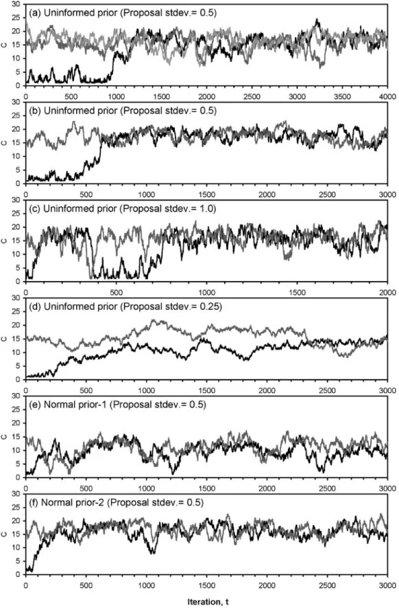
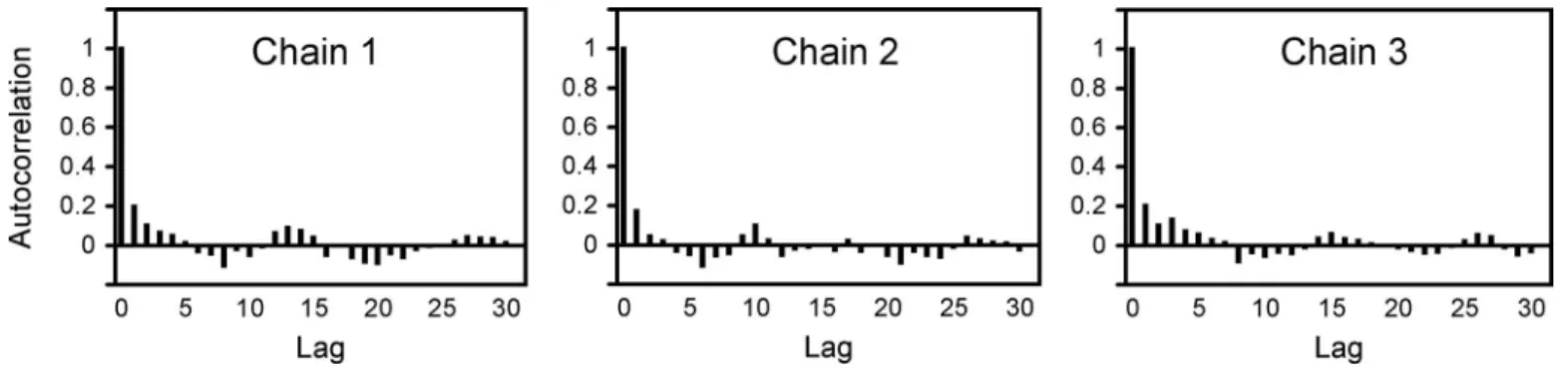
Two- and three-chain MCMC were performed to examine whether using different numbers of chains would result in differ-ent outcomes. The starting values used in the two-chain MCMC were 1 and 15关Fig. 2共b兲兴, whereas an extra starting value of 25 was used in the three-chain MCMC关Fig. 2共a兲兴. Here, for simplic-ity, a single set of data共C-5兲 was used as the input. Chains were run for sufficiently long to confirm that they had indeed con-verged. The evolution of R 共PSRF兲 to unity is shown in Fig. 3, where it is demonstrated that two-chain MCMC reached equilib-rium after approximately 1,000 iterations, whereas the three chains required more than 1,500 iterations to be fully mixed. The faster convergence of two-chain MCMC was also observed in Fig. 2共b兲, as compared to the three chains shown in Fig. 2共a兲. To further examine the efficient mixing of sampler output, the lag-autocorrelations for each line of the three chains共Fig. 4兲 demon-strate that the autocorrelations within each chain were practically negligible and confirm that convergence was efficient.

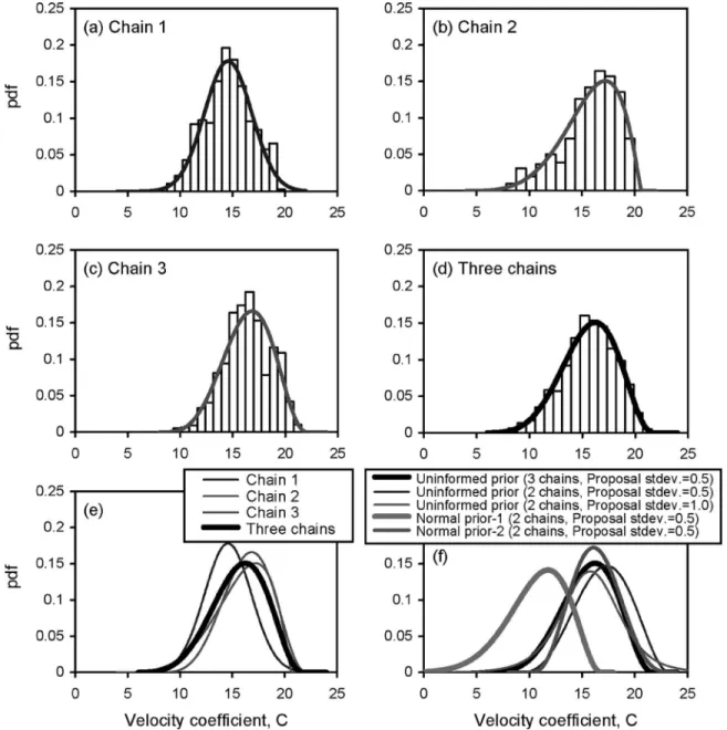
The posterior histograms for each line of the three chains are shown in Figs. 5共a–c兲, and the histogram derived from all three lines is shown in Fig. 5共d兲, where the corresponding best-fit PDF are Normal共14.6, 4.8兲, BetaGeneral共6.0, 2.2, 2.4, 20.6兲, BetaGen-eral共5.6, 3.7, 7.5, 22.2兲, and BetaGeneral共6.6, 3.6, 4.3, 21.9兲, re-spectively. These posterior PDF are all plotted in Fig. 5共e兲 for an overall comparison. Although the posterior PDF of chain 1 was less similar to the other two, the three-chain PDF eliminated in-dividual differences and may well represent the distribution pat-tern of the entire sampler output. The posterior PDFs of two- and three-chain MCMC are shown in Fig. 5共f兲, where the best-fit PDF resulting from two-chain MCMC, i.e., BetaGeneral共4.2, 3.3, 8.9, 23.4兲, slightly deviated from the three-chain PDF in the location of mode共17.3 versus 16.2兲, but had an identical probability den-sity共=0.15兲 at the mode. These results suggest that the outcomes of two- and three-chain MCMC were, practically speaking, not significantly different. Thus, throughout this study we use two chains to perform MCMC.

Scale Factor of Proposal Distribution

Three values of s共i.e., 0.25, 0.5, and 1.0兲 were used to explore the influence of scale factor on the outcomes of MCMC. Two-chain simulations were carried out using an uninformed prior. The sam-pler outputs are shown in Figs. 2共b–d兲, with the corresponding evolutions of PSRF demonstrated in Fig. 3. The sampler output associated with s = 1.0 reached equilibrium after approximately 1,500 iterations, whereas the sampler output associated with s = 0.25 exhibited very slow mixing and the convergence criterion was almost reached after 3,000 iterations. Both of these sampler outputs, however, mixed more slowly than the output associated with s = 0.5, which confirmed that a scale factor too cautious or too bold would result in slow convergence.

The posterior PDF of the sampler outputs associated with s = 0.5 and 1.0 are demonstrated in Fig. 5共f兲, the functional form

Table 1. Compiled Data from Gravel-Bed Experiments

Run ␶0共Pa兲 ks + _D i共mm兲 pi共%兲 ETi C-2 2.16 740 1.68 1.3 2.59 6.6 3.67 11.8 5.04 10.7 7.78 39.3 11 30.3 0.018 C-3 3.76 1,040 1.68 0.9 0.176 2.59 6.1 0.138 3.67 5.8 0.096 5.04 9.6 0.061 7.78 40.6 0.058 11 37.1 C-4 3.08 940 1.68 0.8 2.59 8.7 3.67 8.2 5.04 8.8 0.021 7.78 39.5 11 33.9 C-5 4.46 1,130 1.68 0.8 0.229 2.59 7.7 0.164 3.67 7.2 0.113 5.04 8.6 0.087 7.78 39.2 0.039 11 36.5 0.033 C-6 4.75 1,200 1.68 0.8 0.306 2.59 9.4 0.229 3.67 5.7 0.171 5.04 7.6 0.133 7.78 36.2 0.057 11 40.2 0.043 C-7 4.06 1,080 1.68 1.7 0.177 2.59 13.4 0.144 3.67 11 0.107 5.04 9.7 0.082 7.78 34.3 0.065 11 29.8 0.055

of the latter is Logistic共15.8, 1.8兲. The PDF of the sampler output associated with s = 0.25 is not shown because it had not fully converged. Practically speaking, the difference between the pos-terior PDF associated with s = 0.5 and 1.0 was not significant, with their modes located at 17.3 and 15.8, and the corresponding prob-ability densities being 0.15 and 0.14, respectively. The results suggest that the scale factor of proposal affects significantly the rate of convergence, but not so pronouncedly the posterior distributions.

Prior Distribution

Two alternative priors, i.e., a semiinformed normal prior N共8.05,3.1兲 with its mean and variance derived from the reported lower and upper bounds共Nikora et al. 2001兲 and a normal poste-rior N共17.3,5.5兲 resulting from uninformed prior, were used for exploring the effect of prior on the outcomes of MCMC. The sampler outputs resulting from these alternative priors共denoted as normal prior-1 and prior-2, respectively兲 are shown in Figs. 2共e and f兲, which are to be compared with the output resulting from

Table 2. Compiled Data from Experiments with Four Types of Sediment Mixture

Sediment mixture ␶0共Pa兲 ks

+ Di共mm兲 pi共%兲 ETi Type 1 0.57 26 0.64 28 0.73 30 0.22 6 0.715 0.753 0.793 0.27 6 0.676 0.719 0.764 0.35 14 0.627 0.674 0.726 0.45 12 0.566 0.619 0.678 0.55 12 0.513 0.57 0.635 0.69 12 0.449 0.51 0.58 0.89 8 0.377 0.44 0.515 1.22 8 0.287 0.35 0.429 1.73 5 0.196 0.253 0.33 2.45 5 0.12 0.167 0.235 Type 2 1.11 36 0.86 32 1.1 36 0.22 6 0.879 0.831 0.877 0.27 6 0.861 0.808 0.86 0.35 14 0.839 0.776 0.837 0.45 12 0.81 0.736 0.807 0.55 10 0.783 0.700 0.780 0.69 11 0.747 0.653 0.744 0.89 8 0.702 0.595 0.699 1.22 9 0.638 0.516 0.634 1.73 4 0.556 0.42 0.552 2.45 5 0.464 0.321 0.459 Type 3 1.55 41 1.26 37 0.22 6 0.918 0.895 0.27 6 0.907 0.881 0.35 14 0.892 0.861 0.45 12 0.873 0.837 0.55 4 0.855 0.813 0.69 14 0.832 0.783 0.89 2 0.801 0.744 1.22 9 0.756 0.687 1.73 7 0.696 0.613 2.45 4 0.624 0.527 Type 4 1.6 56 0.22 3 0.906 0.27 8 0.894 0.35 7 0.877 0.45 8 0.855 0.55 5 0.835 0.69 9 0.807 0.89 4 0.773 1.22 9 0.722 1.73 7 0.654 2.45 11 0.575

Fig. 2. Sampler outputs of velocity coefficient C resulting from univariate MCMC using共a兲 three chains, uninformed prior, and proposal scale

factor= 0.5;共b兲 two chains, uninformed prior, and proposal scale factor=0.5; 共c兲 two chains, uninformed prior, and proposal scale factor=1.0; 共d兲 two chains, uninformed prior, and proposal scale factor= 0.25;共e兲 two chains, normal prior N共8.05,3.1兲, and proposal scale factor=0.5; and 共f兲 two chains, normal prior N共17.3,5.5兲, and proposal scale factor=0.5

uninformed prior 关Fig. 2共b兲兴. The results revealed that conver-gence of sampler outputs was achieved much faster as normal priors were used. For both of the simulations using normal priors, equilibrium was reached prior to 500 iterations共Fig. 3兲. Although normal prior-1 and prior-2 were different in values of mean and variance, their output results consistently demonstrated better convergence than the output resulting from uninformed prior.

The posterior distributions resulting from normal prior-1 and prior-2 are demonstrated in Fig. 5共f兲 along with other posteriors discussed earlier. The posterior PDF resulting from normal prior-1 and prior-2, i.e., BetaGeneral共11.5, 3.5, -10.0, 16.9兲 and BetaGeneral共4.3, 5.2, 10.0, 24.0兲, were significantly different, with their modes located at 11.8 and 16.1, and the corresponding probability densities being 0.14 and 0.17, respectively. It is specu-lated that the smaller posterior mode resulting from normal prior-1 was mainly attributed to its smaller prior mode 共=8.05兲, whereas the greater posterior mode resulting from normal prior-2 was attributable to its greater prior mode 共=17.3兲. Further, the highest probability density corresponding to the posterior mode was observed for the outcome resulting from an informed prior 共i.e., normal prior-2兲. As this informed prior was a posterior of uninformed prior, the posterior of normal prior-2 was also similar to those resulting from uninformed priors. However, the highest probability density corresponding to the posterior mode may imply that uncertainty reduction was enhanced by incorporating more prior information.

The results suggest that convergence of sampler outputs is achieved faster if informed priors are used. The posterior

distri-butions are significantly affected by input priors, and parameter uncertainty is reduced as informed priors are incorporated into the MCMC.

Correlation Coefficient of the GC Joint PDF

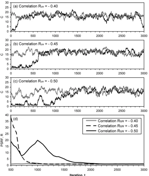
Three typical values of Ruv共i.e., −0.4, −0.45, and −0.5兲 were used

to examine whether the outcomes of MCMC were influenced by the correlation coefficient of the GC joint PDF. The scale factor s = 0.5 and uninformed prior were used in these simulations. The sampler outputs resulting from these values of Ruvare shown in

Figs. 6共a–c兲, with the corresponding evolution of PSRF given in Fig. 6共d兲. Convergence of the sampler output resulting from Ruv= −0.4 was the fastest共convergence criterion was met prior to

500 iterations兲, whereas convergence of the sampler output result-ing from Ruv= −0.5 was the slowest 共convergence criterion was

met after 2,000 iterations兲. The results indicate that if streamwise and vertical fluctuations are more correlated, a greater number of iterations are required to reach a stationary posterior. Such an outcome was probably due to the correlation between streamwise and vertical fluctuations being a constraint imposed on MCMC. Given a higher Ruv, the values of u⬘andv⬘would be restricted in

narrower ranges such that a more suitable value of C must be drawn from the proposal to yield an acceptance probability␣ that would allow the chains to move forward.

The posterior distributions of the sampler outputs resulting from three values of Ruvare shown in Fig. 7, where the best-fit

PDF for Ruv= −0.4 and −0.5 were Logistic共16.0, 1.2兲 and

BetaGeneral共8.1, 4.4, 4.9, 22.5兲, respectively. The results given in Figs. 6 and 7 revealed that the rate of convergence does not nec-essarily coincide with the degree of uncertainty reduction. With an uninformed prior used in these runs, the reduction of parameter uncertainty may be evaluated with the shape of the posterior. The posterior PDF resulting from Ruv= −0.4 had a highest probability

density 共=0.21兲 corresponding to its mode 共=16.0兲, whereas the posterior PDF resulting from Ruv= −0.45 had a lowest probability

density共=0.15兲 corresponding to its mode 共=17.3兲. The posterior PDF resulting from Ruv= −0.5 had a probability density of 0.17

corresponding to its mode at 16.8, both the mode and probability density were between those values associated with Ruv= −0.4 and

−0.45. Because Ruv and C are both physical parameters of the

sediment entrainment model rather than stochastic parameters of MCMC, we speculate that the outcomes shown in Fig. 7 were related to the physical setting of the experiment, i.e., for Run C-5 the near-bed values of Ruv were probably most dominated by

those close to −0.4 and least dominated by those close to −0.45.

Fig. 3. Evolutions of potential scale reduction factor共PSRF兲 R for

sampler outputs shown in Fig. 2

As Ruvvaries as a function of local turbulence and bed

character-istics that is not fully understood at this moment共Wu and Jiang 2007兲, throughout this study a constant value of Ruv= −0.45 was

used, leaving a largest uncertainty in C to be resolved via multiple-input and multivariate Bayesian updating.

Number of Input Data

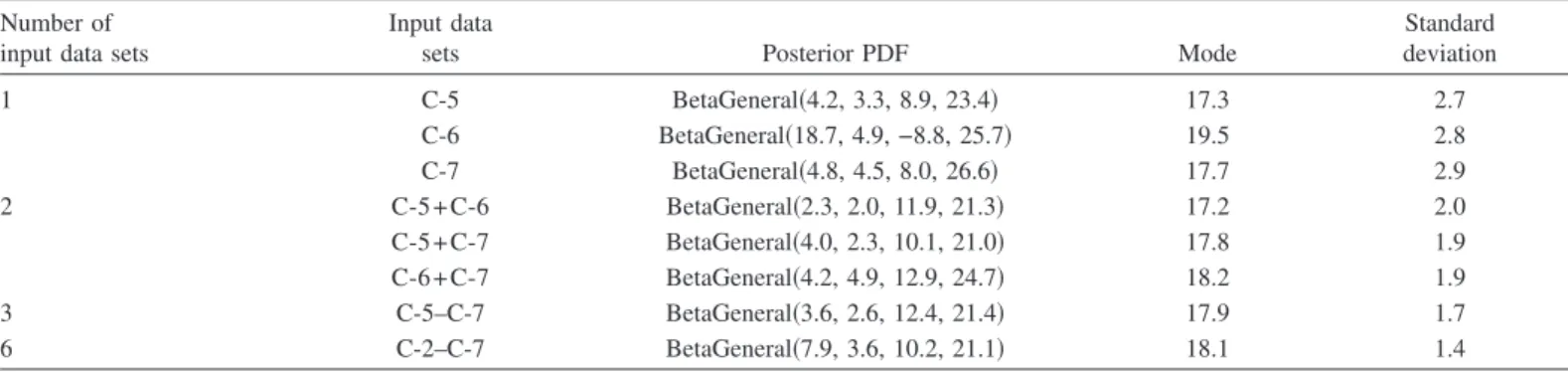
Bayesian updating depends crucially on additional data available, thus the number of input data should have an important influence on the results of MCMC. To explore this, we used one set of data 共C-5, C-6, or C-7兲, two sets of data 共C-5+C-6, C-5+C-7, or C-6 + C-7兲, three sets of data 5–C-7兲, and six sets of data 共C-2–C-7兲 as the inputs to MCMC. The scale factor s=0.5 and un-informed prior were used in these simulations. The posterior PDF resulting from different numbers of input data sets are shown in Fig. 8 and Table 3, with the posterior modes and standard devia-tions also listed in Table 3. Generally, the posterior PDF were distributed in much narrower ranges if more than two sets of input

data were used. For the posterior PDF resulting from one set of input data, the modes ranged between 17.3 and 19.5, with the standard deviations consistently greater than 2.7. For the posterior PDF resulting from two data sets, the modes were concentrated in the range between 17.2 and 18.2, with the standard deviations reduced to the values less than 2.0. As the number of data sets increased from 3 to 6, the posterior mode varied slightly from 17.9 to 18.1, with the standard deviation further reduced to 1.4. These results indicate that the parameter uncertainty reduces with increasing number of input data. So far, MCMC simulations were carried out to update a single parameter C. The values of C de-rived from univariate MCMC were, however, consistently greater than those reported by previous investigators 共e.g., Ligrani and Moffat 1986; Bandyopadhyay 1987; Bridge and Bennett 1992; Nikora et al. 2001; Wu and Yang 2004a兲, which may indicate that larger C values would be obtained when the other parameters remain fixed, and also raise the need to perform multivariate Bayesian updating.

Fig. 5. Posterior histograms and best-fit PDFs of the three chains shown in Fig. 2共a兲 are demonstrated individually and collectively in 共a兲–共e兲 for

Multivariate Bayesian Updating

Multivariate MCMC simulations were carried out in this study to simultaneously update the velocity coefficient C and statistical moments of the GC joint pdf. To accelerate the rate of conver-gence, here a normal posterior N共17.3,5.5兲, derived using unin-formed prior and single input data set共C-5兲, was used as the prior of C 共note that this normal PDF was used earlier as an alter-native prior兲, and a normal joint PDF was used as the prior of the statistical moments, with the mean vector and variance ma-trix specified in Eq. 共9兲. The starting values were taken to be 共prior mean兲⫾共5⫻prior standard deviation兲. For ␴u/u_* and

␴v/u_*, however, the lower chain was started with 共prior

mean兲+共3⫻prior standard deviation兲, such that negative values could be avoided. The likelihood and proposals were those speci-fied in Eqs.共10兲 and 共11兲, with s=0.5 used in Eq. 共11a兲. The full set of gravel-bed data 共i.e., C-2–C-7兲 were used to update the

Fig. 6. Sampler outputs of velocity coefficient C resulting from correlation coefficient Ruv= −0.4, −0.45, and −0.5 are shown in共a兲–共c兲; evolutions

of potential scale reduction factor共PSRF兲 R are shown in 共d兲

Fig. 7. Best-fit posterior PDFs of the sampler outputs shown in

parameters in rough regimes, whereas the compiled data given in Table 2 were used to update the parameters in transitional regimes.

For fully rough flows, the sampler outputs of all seven param-eters are shown in Fig. 9, with the marginal priors and posteriors demonstrated in Fig. 10. The functional forms of posterior PDF are given in Table 4; the prior and posterior standard deviations are also given for a comparison. The distribution of C was sig-nificantly modified via multivariate MCMC, with the mode shifted from 17.3 to 10.8 and standard deviation reduced from 2.345 to 0.815, implying some 65% reduction in uncertainty. Modifications in the distributions of six statistical moments were, however, more limited, with the reductions in standard deviation ranging from 2 to 13%. Two exceptions were observed for Suand

Sv whose posterior standard deviations were greater than their

prior values, implying that underestimation of prior uncertainties was likely to occur if sparse data were available.

For transitional regimes, C varies as a function of k_s+, thus the compiled data sets were used each at a time as the input to MCMC for updating the parameters associated with each k_s+. The posterior modes and standard deviations resulting from multivari-ate MCMC are shown in Table 5, where the posterior standard deviations of C resulting from univariate MCMC are given for a comparison. The posterior modes and 90% confidence intervals of C resulting from univariate and multivariate MCMC are also demonstrated in Fig. 11 along with the results of several previous studies, including those of Ligrani and Moffat 共1986兲, Bandyo-padhyay 共1987兲, Bridge and Bennett 共1992兲, and Wu and Yang 共2004a兲. Among these, the first three were derived for transitional

flows, and it was suggested that C remains constant in fully rough flows; the last one was empirically derived from a compiled data set with k_s+⬍1,000. As shown, the first three exhibit an increasing trend of C followed by a decrease within transitional regimes, and then remain constant in fully rough regimes, whereas the last one decreases monotonically with k_s+.

Fig. 11 demonstrates that the rough-regime values of C result-ing from multivariate MCMC were more consistent with three

Fig. 8. Best-fit posterior PDFs of velocity coefficient C resulting

from different input data sets

Table 3. Posterior Distributions, Modes, and Standard Deviations of Velocity Coefficient Resulting from Univariate MCMC with Different Numbers of

Input Data Sets Number of input data sets

Input data

sets Posterior PDF Mode

Standard deviation 1 C-5 BetaGeneral共4.2, 3.3, 8.9, 23.4兲 17.3 2.7 C-6 BetaGeneral共18.7, 4.9, −8.8, 25.7兲 19.5 2.8 C-7 BetaGeneral共4.8, 4.5, 8.0, 26.6兲 17.7 2.9 2 C-5 + C-6 BetaGeneral共2.3, 2.0, 11.9, 21.3兲 17.2 2.0 C-5 + C-7 BetaGeneral共4.0, 2.3, 10.1, 21.0兲 17.8 1.9 C-6 + C-7 BetaGeneral共4.2, 4.9, 12.9, 24.7兲 18.2 1.9 3 C-5–C-7 BetaGeneral共3.6, 2.6, 12.4, 21.4兲 17.9 1.7 6 C-2–C-7 BetaGeneral共7.9, 3.6, 10.2, 21.1兲 18.1 1.4

Fig. 9. Sampler outputs of velocity coefficient C and six statistical

moments of the GC PDF resulting from multivariate MCMC using rough-regime data

previous results, whereas those resulting from univariate MCMC were much greater. The 90% confidence interval resulting from multivariate MCMC was 43% smaller than that resulting from univariate MCMC. For transitional regimes, the discrepancies be-tween the outcomes of univariate and multivariate MCMC were not as significant as those for rough regimes, with the reductions in standard deviations ranging from 8 to 35%共Table 5兲, implying that an average of 22% reduction in uncertainty was achieved by multivariate MCMC. It is also revealed in Fig. 11 that the transitional-regime posterior modes exhibited a variation trend similar to those of three previous results, i.e., an initial increasing trend with k_s+ followed by a decreasing one. However, the varia-tion trend of the posterior modes was much steeper. For 32⬍k_s+ ⬍70, the posterior values of C were consistently greater than previous results; for 28⬍k_s+⬍32, the posterior values appeared to coincide with three previous results; whereas for k_s+⬍28, the pos-terior values were much closer to the result of Wu and Yang 共2004a兲.

For transitional regimes, the posterior modes and standard de-viations of the four statistical moments共Table 5兲 revealed that the differences between prior and posterior modes were almost

neg-ligible. The changes between prior and posterior standard devia-tions were also limited, with the average changes ranging between −4 and −11%. Compared to the above-mentioned 22% reduction in the uncertainty of C, the modifications in the transitional-regime statistical moments were rather modest, simi-lar to the situations observed for rough regimes. However, in-creases in the posterior standard deviations were observed sporadically, which again could be attributed to the sparse data available for estimating the prior uncertainties.

Application to Prediction of Entrainment Probabilities

In this section, the updated parameters were applied in the sedi-ment entrainsedi-ment model to demonstrate their practical effect on the prediction of entrainment probabilities. To this end, the modes of the prior and posterior distributions were used separately as the parameter values for numerical simulations. For the coefficient C, the mode of the normal prior N共8.05,3.1兲 was used as the prior parameter, whereas the posterior modes resulting from multivari-ate MCMC共see Fig. 11兲 were used as the posterior parameters for different values of k_s+. For the statistical moments of the GC joint

Table 4. Posterior Distributions of Parameters Resulting from Multivariate MCMC and Comparison of Prior and Posterior Standard Deviations共for Fully

Rough Flows兲

Parameter Posterior PDF

Standard deviation

Prior Posterior 共Changea兲

C BetaGeneral共10.9, 12.8, 7.1, 15.2兲 2.345 0.815 共−65%兲 ␴u/u_* BetaGeneral共19.3, 13.8, 1.8, 2.3兲 0.046 0.040 共−13%兲 ␴v/u_* Weibull共4.2, 0.84兲 0.237 0.206 共−13%兲 Su Normal共0.40, 0.15兲 0.134 0.154 共+15%兲 Sv BetaGeneral共3.6, 5.4, −0.74, 1.1兲 0.232 0.278 共+20%兲 M21 Normal共−0.090, 0.093兲 0.100 0.093 共−7%兲 M12 Weibull共3.6, 0.18兲 0.051 0.050 共−2%兲 a

Percentage change between prior and posterior standard deviations.

Table 5. Posterior Modes and Standard Deviations of Parameters Resulting from Multivariate MCMC共for Transitional Flows兲

Parameter Prior Posterior for k_s+₌ 26 28 30 32 36 37 41 56 C Std. Deva 0.773 1.007 0.839 1.071 1.203 2.053 3.048 1.224 Std. Devb 0.636 0.657 0.588 0.789 0.830 1.805 2.669 1.124 共Changec_{兲 共−18%兲 共−35%兲 共−30%兲 共−26%兲 共−31%兲 共−12%兲 共−12%兲 共−8%兲} ␴v/u_* Mode 0.99 0.97 0.94 0.97 1.05 1.04 0.97 1.04 0.96 Std. dev. 0.237 0.189 0.240 0.168 0.282 0.280 0.204 0.237 0.213 共Changed_{兲 共−20%兲 共+1%兲 共−29%兲 共+19%兲 共+18%兲 共−14%兲 共0%兲 共−10%兲} Sv Mode −0.01 −0.01 0.00 −0.01 0.01 −0.01 0.00 0.00 0.00 Std. dev. 0.233 0.222 0.219 0.221 0.191 0.183 0.283 0.196 0.225 共Changed 兲 共−5%兲 共−6%兲 共−5%兲 共−18%兲 共−21%兲 共+21%兲 共−16%兲 共−3%兲 M21 Mode −0.07 −0.07 −0.08 −0.06 −0.13 −0.08 −0.05 −0.07 −0.09 Std. dev. 0.100 0.090 0.089 0.079 0.091 0.087 0.097 0.096 0.082 共Changed_{兲 共−10%兲 共−11%兲 共−21%兲 共−9%兲 共−13%兲 共−3%兲 共−4%兲 共−18%兲} M12 Mode 0.12 0.13 0.11 0.11 0.14 0.11 0.11 0.13 0.12 Std. dev. 0.051 0.049 0.059 0.047 0.037 0.055 0.042 0.049 0.039 共Changed 兲 共−4%兲 共+16%兲 共−8%兲 共−27%兲 共+8%兲 共−18%兲 共−4%兲 共−24%兲

Note: Posterior standard deviations of coefficient C resulting from univariate MCMC are also listed for comparison.

a

Posterior standard deviation resulting from univariate MCMC.

b

Posterior standard deviation resulting from multivariate MCMC.

c

Percentage change between univariate and multivariate posterior standard deviations.

d

PDF, the modes 共or means兲 given in Eq. 共9a兲 were used as the prior parameters, whereas the posterior modes shown in Fig. 10 and Table 5 were used as the posterior parameters for rough and transitional regimes, respectively. Comparisons of the predicted and observed entrainment probabilities are illustrated in Fig. 12, where the outcomes resulting from prior and posterior parameters are demonstrated. The entrainment probabilities predicted using the posterior parameters were more consistent with the observed data, whereas the predicted entrainment probabilities associated with prior parameters were consistently lower than the observed values. Such a result was probably due to a small value of C 共=8.05兲 used as the prior parameter, given the fact that the poste-rior modes of C deviated substantially from this pposte-rior value but the posterior modes of the statistical moments were not signifi-cantly different from their prior values. With the parameters up-dated for rough and transitional regimes, the sediment entrainment model was able to compute more accurately and re-alistically the entrainment probabilities. The global coefficient of determination R2_{increased from 0.76 to 0.91 as the prior}

param-eters were replaced by the posterior ones, which implied a 20% improvement in the accuracy of predictions.

Conclusions

This work presents a Bayesian framework using MCMC to up-date the parameters of a sediment entrainment model. In the first part of this paper, univariate MCMC sensitivity analyses were performed using different numbers of chains, scale factors of pro-posal, prior distributions, correlation coefficients, and numbers of input data. The results reveal that the outcomes of two- and three-chain MCMC were, practically speaking, not significantly differ-ent. Convergence of two-chain MCMC was, however, faster than that of three-chain MCMC. The results confirmed that a scale factor too cautious or too bold would result in slow convergence. The results also suggested that the scale factor significantly

af-fects the rate of convergence but not the posterior distributions. The sampler outputs of MCMC using informed priors converge much faster than those using an uninformed prior. The posterior distributions are significantly influenced by the patterns of priors, and the reduction of parameter uncertainty is enhanced by in-formed priors. The correlation coefficient of the GC PDF is a physical parameter related to the specific setting of experiments, hence is a physical constraint imposed on MCMC in which a higher correlation would require a greater number of iterations to fully mix the chains. Our results indicate that the parameter un-certainty reduces with increasing number of input data sets. The posterior PDF are generally distributed in much narrower ranges if more than two sets of input data are used.

In the second part of this study, multivariate MCMC were carried out to simultaneously update the velocity coefficient C and the statistical moments of the GC PDF. For fully rough re-gimes, the distributions of C 共mean and variance兲 were signifi-cantly modified via multivariate MCMC. For transitional regimes, the differences between the posterior values of C resulting from univariate and multivariate MCMC were not as significant as

Fig. 11. Posterior modes and 90% confidence intervals of velocity

coefficient C resulting from univariate and multivariate MCMC. Compiled data shown in Table 2 were used for updating the constant value of C in rough regimes共k_s+艌70兲, whereas compiled data shown in Table 3 were used for updating the variation trend of C in transi-tional regimes共k_s+⬍70兲. Symbols and error bars denote the modes and 90% confidence intervals, respectively. Gray error bars are with empty symbols, whereas black error bars are with solid symbols. Results of four previous studies are shown for comparison.

Fig. 12. Comparisons of observed data and predicted entrainment

those for rough regimes. The posterior values of C exhibited a similar but steeper variation trend compared to those of previous results. For both rough and transitional regimes, the differences between the prior and posterior distributions of the statistical mo-ments were, however, rather limited.

In the last part of this study, the practical effect of updated parameters on the prediction of entrainment probabilities was demonstrated. The entrainment probabilities predicted using the updated parameters were more consistent with the observed val-ues. With all the parameters updated via MCMC, the sediment entrainment model was able to compute more accurately and re-alistically the entrainment probabilities.

Acknowledgments

This study was supported in part by the National Science Council of Taiwan ROC. Comments from the editors and two anonymous reviewers helped to improve the clarity and completeness of this presentation.

Notation

The following symbols are used in this paper: C ⫽ velocity profile coefficient; Di ⫽ grain size of the ith fraction;

D50 ⫽ median grain size;

d ⫽ m⫻n matrix of observed data;

ETi ⫽ observed entrainment probabilities of the ith

size fraction;

g共U,V兲 ⫽ third-order Gram–Charlier joint PDF; i ⫽ size fraction index;

j ⫽ chain index; k ⫽ observation index;

ks ⫽ equivalent roughness height=2D50;

k_s+ _{⫽ roughness Reynolds number=u} *ks/␯;

L1– L4 ⫽ third-order expansion of Hermite polynomials

defined in Eq.共4兲; M21, M12 ⫽ diffusion factors;

m ⫽ number of observations;

n ⫽ number of data in each observation 共=total number of size fractions兲;

P共␪兲 ⫽ prior distribution of ␪;

P共d兩␪兲 ⫽ likelihood function of d under condition ␪; P共␪兩d兲 ⫽ posterior distribution of ␪ given dada d;

PTi ⫽ expected entrainment probability for the ith

size fraction;

pi ⫽ proportion of the ith size fraction;

q共␪_*兩␪t兲 ⫽ proposal distribution;

R ⫽ potential scale reduction factor 共PSRF兲; Ru ⫽ RuvU − V;

Ruv ⫽ u⬘v⬘/␴u␴v= correlation coefficient of the GC

joint PDF; Rv ⫽ RuvV − U;

Su, Sv ⫽ skewness factors;

s ⫽ scale factor of proposal distribution; t ⫽ iteration index;

U ⫽ u⬘/␴u;

u⬘,v⬘ ⫽ streamwise and vertical velocity fluctuations,

respectively;

u_* ⫽ bed shear velocity =冑␶_0/␳;

u

¯共y兲 ⫽ time-averaged streamwise velocity at a height y from the origin;

V ⫽ v⬘/␴v;

␣ ⫽ acceptance probability;

␦ ⫽ thickness of the roughness layer;

␨ ⫽ random sample drawn from Uniform共0, 1兲; ␬ ⫽ von Karman constant=0.4;

␮prior ⫽ prior mean vector of ␪6;

␯ ⫽ kinematic viscosity of fluid; ␪ ⫽ parameter vector;

␪t ⫽ tth realization of parameter vector;

␪_* ⫽ candidate parameter vector; ␪6 ⫽ parameters of the GC PDF

=关␴u/u_*,␴v/u_*, Su, Sv, M21, M12兴T;

␳ ⫽ density of fluid; ⌺UV ⫽ covariance matrix;

⌺prior ⫽ prior covariance matrix of ␪6;

␴u,␴v ⫽ standard deviations of u⬘andv⬘;

␴2 _{⫽ variance quantifying model errors; and}

␶0 ⫽ bed shear stress.

References

Balakrishnan, S., Roy, A., Ierapetritou, M. G., Flach, G. P., and Geor-gopoulos, P. G.共2003兲. “Uncertainty reduction and characterization for complex environmental fate and transport models: An empirical Bayesian framework incorporating the stochastic response surface method.” Water Resour. Res., 39共12兲.

Bandyopadhyay, P. R.共1987兲. “Rough-wall turbulent boundary layers in the transitional regime.” J. Fluid Mech., 180, 231–266.

Box, G. E. P.共1980兲. “Sampling and Bayes’ inference in scientific mod-elling and robustness共with discussion兲.” J. R. Stat. Soc. Ser. A (Gen.),

143, 383–430.

Bridge, J. S., and Bennett, S. J.共1992兲. “A model for the entrainment and transport of sediment grains of mixed sizes, shapes, and densities.”

Water Resour. Res., 28共2兲, 337–363.

Brooks, S., and Gelman, A. 共1998兲. “General methods for monitoring convergence of iterative simulations.” J. Comput. Graph. Stat., 7, 434–455.

Draper, D.共2006兲. Bayesian hierarchical modeling, Springer, New York. Gamerman, D., and Lopes, H. F. 共2006兲. Markov chain Monte Carlo:

Stochastic simulation for Bayesian inference, Chapman and Hall/

CRC, Boca Raton, Fla.

Gelfand, A. E., and Smith, A. F. M.共1990兲. “Sampling-based approaches to calculating marginal densities.” J. Am. Stat. Assoc., 85, 399–409. Gelman, A., Carlin, J. B., Stern, H. S., and Rubin, D. B.共2004兲. Bayesian

data analysis, Chapman and Hall/CRC, Boca Raton, Fla.

Gilks, W. R., Richardson, S., and Spiegelhalter, D. J., eds.共1996兲.

Mar-kov chain Monte Carlo in practice, Chapman and Hall, London.

Ligrani, P. M., and Moffat, R. J.共1986兲. “Structure of transitionally rough and fully turbulent boundary layers.” J. Fluid Mech., 162, 69–98. Marshall, L., Nott, D., and Sharma, A.共2004兲. “A comparative study of

Markov chain Monte Carlo methods for conceptual rainfall-runoff modeling.” Water Resour. Res., 40.

Metropolis, N., Rosenbluth, A., Rosenbluth, M., Teller, A., and Teller, E. 共1953兲. “Equations of state calculations by fast computing machines.”

J. Chem. Phys., 21, 1087–1092.

Nikora, V. I., Goring, D. G., McEwan, I., and Griffiths, G.共2001兲. “Spa-tially averaged open-channel flow over rough bed.” J. Hydraul. Eng.,

127共2兲, 123–133.

Pope, S. B.共2000兲. Turbulent flows, Cambridge University Press, New York.

Reis, D. S., and Stedinger, J. R.共2005兲. “Bayesian MCMC flood fre-quency analysis with historical information.” J. Hydrol., 313, 97–116.

Renard, B., Garreta, V., and Lang, M.共2006兲. “An application of Baye-sian analysis and Markov chain Monte Carlo methods to the estima-tion of a regional trend in annual maxima.” Water Resour. Res., 42. Rubin, D. B.共1984兲. “Bayesianly justifiable and relevant frequency

cal-culations for the applied statistician.” Ann. Stat., 12, 1151–1172. Smith, B. J. 共2005兲. “Bayesian output analysis program 共BOA兲 version

1.1 user’s manual.” Dept. of Biostatistics, Univ. of Iowa, College of Public Health,具http://www.public-health.uiowa.edu/boa典.

Spall, J. C.共2003兲. “Estimation via Markov chain Monte Carlo.” IEEE

Control Syst. Mag., 34–45.

Sun, Z., and Donahue, J.共2000兲. “Statistically derived bedload formula

for any fraction of nonuniform sediment.” J. Hydraul. Eng., 126共2兲, 105–111.

Wu, F.-C., and Jiang, M.-R.共2007兲. “Numerical investigation of the role of turbulent bursting in sediment entrainment.” J. Hydraul. Eng.,

133共3兲, 329–334.

Wu, F.-C., and Yang, K.-H.共2004a兲. “Entrainment probabilities of mixed-size sediment incorporating near-bed coherent flow structures.” J.

Hy-draul. Eng., 130共12兲, 1187–1197.

Wu, F.-C., and Yang, K.-H.共2004b兲. “A stochastic partial transport model for mixed-size sediment: Application to assessment of fractional mo-bility.” Water Resour. Res., 40共4兲.