針對下一世代無線網路所設計之訊框聚合鏈路適應演算法

國 立 交 通 大 學

電信工程學系

碩 士 論 文

針對下一世代無線網路所設計之

訊框聚合鏈路適應演算法

Frame-Aggregated Link Adaptation Algorithm

for Next Generation Wireless Networks

研 究 生：林伯泰 Student:

Po-Tai

Lin

指導教授：方凱田 博士

Advisor: Dr. Kai-Ten Feng

針對下一世代無線網路所設計之

訊框聚合鏈路適應演算法

Frame-Aggregated Link Adaptation Algorithm for Next

Generation Wireless Networks

研 究 生：林伯泰 Student:

Po-Tai

Lin

指導教授：方凱田 博士

Advisor: Dr. Kai-Ten Feng

國立交通大學

電信工程學系碩士班

碩士論文

A Thesis

Submitted to Department of Communication Engineering

College of Electrical Engineering and Computer Engineering

National Chiao Tung University

in Partial Fulfillment of the Requirements

for the Degree of

Master of Science

in

Communication Engineering

September 2008

Hsinchu, Taiwan, Republic of China

針對下一世代無線網路所設計之

訊框聚合鏈路適應演算法

研究生：林伯泰

指導教授：方凱田 博士

國立交通大學電信工程學系碩士班

摘要

鏈路適應在無線網路中是一個非常重要的議題。利用鏈路適應的演算法，無 線通訊系統動態地針對不同的通道條件設定調變模式、傳輸速率或任何可調的系 統參數，藉此得到較未使用任何鏈路適應演算法之系統更佳的效能。本論文目的 在 IEEE 802.11n 標準下制定一個表現佳的鏈路適應演算法。在第一章中，不同的 無線網路、IEEE 802.11 無線區網的演進、各類已存在的鏈路適應演算法以及本 論文提出的訊框聚合鏈路適應(FALA, Frame-Aggregated Link Adaptation)演算 法之概念將被介紹。在第二章節中，對 IEEE 802.11n 標準在媒體存取控制(MAC, Medium Access Control)層、實體(PHY, Physical)層的特性及兩個鏈路適應演算 法有詳細地説明。MAC/PHY 層的位元錯誤率(BER)、系統飽和吞吐量分析以及 FALA 演算法則在第三章節中詳細地被解說。在效能評比的部份，本論文所提之 FALA 演 算法、跨層鏈路適應(CLA, Cross-layer Link Adaptation)演算法以及自動速率 調降(ARF, Auto Rate Fallback)演算法將被比較。最後，結論為本論文所提之 FALA 演算法較已存在的 CLA 及 ARF 演算法有較佳的表現。

Frame-Aggregated Link Adaptation Algorithm for

Next Generation Wireless Networks

Student: Po-Tai Lin

Advisor: Dr. Kai-Ten Feng

Department of Communication Engineering

National Chiao Tung University

Abstract

Link adaptation is an important issue in wireless networks about applying some mechanisms to set different modulation modes or data rates corresponding to different channel conditions dynamically in purpose of performance better than the one without any link adaptation algorithm utilized. In the first chapter, some different wireless networks, evolutions of IEEE 802.11 WLANs, concepts of link adaptation and ideas of the existing/proposed frame-aggregated link adaptation (FALA) algorithm are introduced. In the second chapter, features of IEEE 802.11n medium access control (MAC) and physical (PHY) layer, and two existed link adaptation algorithm will be briefly introduced. In the third chapter, evaluation of bit error rate (BER) in PHY/MAC layer, analysis of saturated goodput, and mechanism of FALA algorithm are illustrated in detail. In performance evaluation, the numerical result is verified with the simulation result, and compared to the existed automatic rate fallback (ARF) and cross-layer link adaptation (CLA) algorithms. Finally, a better performance with FALA algorithm utilized will be shown, and the conclusion will be drew that the proposed FALA algorithm works well in link adaptation and outperforms the existed two algorithms.

Acknowledgement

Firs of all, I would like to express my deepest gratitude to my advisor, Dr. Kai-Ten Feng, for his enthusiastic guidance and great patience. I learn a lot from his positive attitude in way of research and many other areas. Secondly, I really appreciate Dr. Wei-Kua Liao and Dr. Hsi-Lu Chao for serving as my committees. Heartfelt thanks are also offered to all members in the Mobile Intelligent Network Technology Laboratory (MINT Lab) for their constant encouragement and assistance whenever I need.

I would like to show my sincere thanks to my parents for their invaluable care and love. When I was depressed, they comforted and encourage me, and whenever I met difficulty, their heart and mind were always by my side. I also appreciate for their supply to every thing I need without any complaining. Without them, I would not exist in this world. Without them, I would not live to this age. Without them, I would not be here today. Sincerely, it is not enough to give all my appreciation to my dear parents. I would like to attribute all my achievement and honor to them. Thank you mom and dad, I love you forever.

Finally, I appreciate all my true friends for their immediately encouraging when I was down. They let me know that someone other than my parents in this world are caring me, I am not alone to fight. I am willing to share my honor with you guys, thank you every one.

Contents

Chinese Abstract

I

English Abstract

II

Acknowledgement III

Contents IV

List of Figures

VI

Chapter 1 Introduction... 1

Chapter 2 Related Work ... 6

2.1 IEEE 802.11n Standard... 6

2.1.1 Medium Access Control (MAC) and Physical (PHY) Layer Protocols . 6

2.2 Existing Link Adaptation Algorithms ... 13

2.2.1 Automatic Rate Fallback (ARF) Algorithm... 13

2.2.2 MAC and PHY Cross-Layer Link Adaptation (CLA) Algorithm... 15

Chapter 3 Proposed Frame-Aggregated Link Adaptation (FALA)

Algortihm 18

3.2 Detail Description of Proposed FALA Algorithm ... 29

Chapter 4 Performance Evaluation... 35

4.1 Analytical Results ... 35 4.2 Simulation Results ... 37 4.2.1 Simulation Parameters ... 37 4.2.2 Model Validation... 37 4.4.3 Performance Comparison ... 38

Chapter 5 Conclusion ... 44

Bibliography... 45

List of Figures

Figure 2.1: Theoretical goodput upper limit GUL in IEEE 802.11a protocols ignoring

the channel noise... 8

Figure 2.2 : The frame format of A-MPDU... 9

Figure 2.3 : The frame format of A-MSDU... 10

Figure 2.4: Throughput of A-MPDU with different aggregation numbers... 11

Figure 2.5: Throughput of A-MSDU with different aggregation numbers... 11

Figure 2.6: Block Acknowlegement with Selective Repeat. ... 12

Figure 2.7: The schematic digram of RTS/CTS handshake operation... 13

Figure 2.8: Goodput for single mode of eight different MCSs and CLA algorithm. Payload size is 2000 bytes. ... 16

Figure 3.1: Mod./Demod. And Convolution coding blocks in PHY Layer. ... 19

Figure 3.2: The average PHY-layer BER corresponding to given mn is denoted as Pbe(mn)... 21

Figure 3.3: The average MAC-layer BER corresponding to given mn is denoted as Pbe(mn)... 21

collision and noisy channel for DCF function ... 23

Figure 3.5: One-dimensional, simplified backoff model when stage-transstion probability p in Fig. 3.4 is nearly zero ... 26

Figure 3.6: Goodput with m2 applied in cases of MPDU payload size l=l*, l>l*, and l<l*

... 30

Figure 3.7: Maximum goodput and optimal MPDU payload size of mn with optimal

payload size used ... 31

Figure 3.8: The system architecture for MAC and PHY protocols with the proposed FALA algorithm implemented. ... 32

Figure 3.9: The SNR axis is bounded by SNRmin and SNRmax, devided by SNRscale into

nSNR regions. ... 33

Figure 4.1: Goodput with FALA algorithm implemented and eihgt single MCSs ... 36

Figure 4.2: Optimal mn* and l* based on FALA algorithms... 37

Figure 4.3: Comparison of simulation and numerical results in the scenario of nSTA=2

and nMPDU=64. ... 39

Figure 4.4: Performance in goodput of FALA algorithm with payload size from 10 to 5000 bytes available and CLA algorithm with payload size l = 5000 bytes. ... 39

Figure 4.5: Different decisions in MCS versus SNR of FALA and CLA algorithms. ... 40

Figure 4.6: Two-state discrete time Markov chain model for channel variation.. ... 40

Figure 4.7: The first diagram is the channel conditions in different transmission attempts generated by applying the two-state discrete Markov chain model with

Pb,g=0.7. The second and the third one is PHY modes used in every transmission

attempts of ARF and FALA respectively.. ... 42

Figure 4.8: Average goodput of FALA, CLA and ARF under the varying channel with different Pb,g from 0 to 1.. ... 42

Chapter 1

Introduction

Wireless network refers to any type of computer networks using wireless communication technologies in connectivity maintenance and messages exchange between stations over less media, such as infrared, laser, ultrasound, and radio waves. Due to wireless nature, wire-less networks have many advantages against its wired counterpart. The obvious one is that the wireless capable station can preserve its connectivity and functionality in the moving sta-tus because of no wire line constraint. Another one is that users can reduce the installation time since the installation of wire line is harder than that of wireless equipments. In addition, the most attractive one is that utilizing the wireless media instead of wires can resolve the wire line deployment problem of hard-to-reach places like human bodies, outer space, deep water, and dangerous areas. In general, the invention of wireless networks compensates the drawbacks of wired networks.

Depending on the size of wireless coverage, wireless networks can be further divided into five networks: wireless regional area networks (WRANs), wireless wide area networks (WWANs), wireless metropolitan area networks (WMANs), wireless local area networks (WLANs), and wireless personal area networks (WPANs). IEEE Standards Association also establishes five standard series of IEEE 802.22, IEEE 802.20, IEEE 802.16, IEEE 802.11, and

IEEE 802.15 for the corresponding networks. Among these wireless standard series, IEEE 802.11 standard suite is the most famous one because of its remarkable success in design, deployment and business.

IEEE 802.11 standard suite has many amendments mainly including IEEE 802.11a/b/g [1–3] for physical layer extensions, IEEE 802.11e [4] for Quality-of-Service (QoS) support, and IEEE 802.11n [5, 6] for high throughput performance over 100Mbps. The simplicity of the carrier sense multiple access with collision avoidance (CSMA/CA) scheme for the medium access control has contributed to the success of the IEEE 802.11 specifications. The WLAN devices that implement the IEEE 802.11b Physical layer [2] support the data trans-mission rate of 11 Mbps; while the data rate of the IEEE 802.11a PHY technique [1] can sustain up to 54 Mbps with the adoption of the orthogonal frequency-division multiplexing (OFDM) transmission scheme. Moreover, there are increasing demands for high through-put communication devices in order to support multimedia applications, e.g. HDTV and DVD. In order to fulfill the requirement for achieving improved throughput performance, the IEEE 802.11 Task Group N (TGn) enhances the PHY layer data rate to 600 Mbps by adopt-ing advanced communication techniques, such as multi-input multi-output (MIMO) technol-ogy [8]. It is noted that MIMO technique utilizes spatial diversity to improve both the range and spatial multiplexing for achieving higher data rate. However, a serious problem advanced in [7] shows that simply improving the PHY data rate without reducing the MAC/PHY over-head does not help the MAC layer throughput surpass 100Mbps. Accordingly, IEEE 802.11 TGn would further exploit packet aggregation techniques to moderate the drawbacks of the MAC/PHY overhead. Besides throughput improving technologies mentioned as the above, multiple data transmission rates are provided in 802.11 PHYs by employing different modula-tion and channel codding schemes. For example that 8 PHY modes are provided in the IEEE 802.11a PHY [1] with different data transmission rates from 6 Mbps to 54 Mbps, even more modulation modes with different data transmission rates are provided in the IEEE 802.11n

PHY [5].

Link adaptation, or so-called adaptive modulation and coding (AMC), is a concept that some mechanisms established to map the modulation, coding, or other protocol parameters toward the channel conditions such as signal-to-noise ratio (SNR), interference from different transmitters, etc. in wireless communication. Due to the wireless nature, the channel condi-tions may varies over time because of some factors such as weather changing, time-varying interference, or even the mobility of stations. With no any mechanism for link adaptation, a poor performance in efficiency of bandwidth utilization can be found when operating in the channel with serious variation. So it is necessary to design a link adaptation algorithm to have better performance against channel variation.

Before the proposed FALA algorithm, some existing algorithms for link adaptation will be introduced as follows. The automatic rate fallback (ARF) algorithm in [11] uses the MAC protocol parameters to trace the channel conditions and decide the packet transmission rate. Two counters are set to trace the successively received good and missed acknowledgement (ACK) frames respectively, and can be taken as the information of channel conditions. If the number of successively received good ACKs reaches ten or the preset timer expires, the packet transmission rate will be upgrade to a higher level. Oppositely, if the number of successively missed ACKs reaches two, the packet transmission rate will fallback to a lower level. The advantage of utilizing ARF algorithm is that there is no complicated computation needed, only few counters and timers need to be set under the standard of existing MAC and PHY layer. Yet the mechanism in ARF algorithm is delayed adaptation and without consideration of PHY layer information. As a result, the performance reduces as the degree of channel variation raises.

Due to problems of delayed adaptation and poor performance in highly varying channel of ARF mentioned above, the cross-layer link adaptation (CLA) algorithm in [12] and some other similar algorithms in [13,14] are proposed to moderate them. In CLA algorithm, both of

the information in MAC and PHY layer are used in calculation to preestablish a mapping table that maps an optimal modulation and coding scheme (MCS) including the modulation mode, coding rate, and packet transmission rate to a given channel condition, say, SNR. This map-ping table is established before the station starts communicating, and is based on the criterion of maximization of the saturated goodput to find the optimal MCS. Then at the run time, only a simple table-lookup is done to find the optimal MCS corresponding to the estimated SNR. This means that additional computation and operation time needed is quite small, i.e. the CLA algorithm is almost real-time. Being real time, CLA algorithm has high improvement in performance in highly varying channel. With the criterion of goodput maximization, CLA algorithm outperforms ARF algorithm in average saturated goodput. However, in CLA al-gorithm, only some optimal information in PHY layer (i.e. MCS) obtained, no other MAC protocol parameters are used in establishing the mapping table. Besides, the analysis of sat-urated goodput in CLA algorithm is for the distributed coordinate function (DCF) only, the frame aggregation mechanism is not taken into consideration.

Thus, in this work, the saturated goodput analysis in consideration of both the PHY-layer information MCSs and the MAC-layer parameter MPDU payload size will be introduced. Moreover, the A-MPDU frame aggregation scheme in standard of IEEE 802.11n MAC pro-tocol [6] of packet transmission is also taken into consideration in the saturated goodput analysis. Then in the proposed FALA algorithm, a table of optimal MCSs and MPDU pay-load sizes is preestablished based on the criterion of maximum saturated goodput in use of the analysis introduced. In performance comparison, it is easily to find that the proposed FALA algorithm keeps the real-time property and performs well in the adaptability to chan-nel variation shown in the saturated goodput versus a time-varying chanchan-nel condition pattern randomly generated. And it outperforms the existing ARF and CLA algorithms in average saturated goodput. As a result, the proposed FALA algorithm in this work is worthy of being implemented.

The organization of this thesis is as follows. In the chapter of related work, some features in IEEE 802.11n standard MAC/PHY protocols and the existing ARF and CLA algorithm are introduced. Then in the chapter of proposed frame-aggregated link adaptation (FALA) algo-rithm, MAC-layer BER and goodput analysis is shown followed with the detail description of the proposed FALA algorithm. After that, in the chapter of performance evaluation, an example of FALA algorithm implementation is shown in section of analytical results. And performance comparison of ARF, CLA and FALA algorithms will be shown in goodput ver-sus SNR, average goodput under different channel varying degree, and channel adaptability. Finally, the conclusion of this thesis is drawn at the end of it.

Chapter 2

Related Work

In this chapter, some important characteristics in the standard of IEEE 802.11n MAC and PHY protocols [5, 6] such as MAC frame formats, channel access schemes, packet aggrega-tion schemes, and MCS etc. will be presented first. Then after that, ideas and mechanisms of the automatic rate fallback (ARF) [11] and the cross-layer link adaptation (CLA) [12] algorithms will be introduced.

2.1 IEEE 802.11n Standard

2.1.1 Medium Access Control (MAC) and Physical (PHY) Layer

Proto-cols

As mentioned in the chapter of inroduction, there are many techniques developed in PHY layer to improve the packet transmission rate, and protocols in MAC layer to make the good-put being closer to the theoretical limit. Thus, the focus of this section are several mecha-nisms or protocols that will be involved in the analysis and simulations of the proposed FALA algorithm.

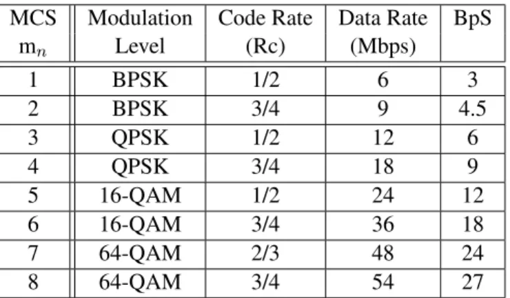
MCS Modulation Code Rate Data Rate BpS mn Level (Rc) (Mbps) 1 BPSK 1/2 6 3 2 BPSK 3/4 9 4.5 3 QPSK 1/2 12 6 4 QPSK 3/4 18 9 5 16-QAM 1/2 24 12 6 16-QAM 3/4 36 18 7 64-QAM 2/3 48 24 8 64-QAM 3/4 54 27

Table 2.1: OFDM Modulation and Coding Schemes of Legacy IEEE 802.11a PHY

raise the packet transmission rate except the MIMO and OFDM techniques mentioned before. For example that more sub-carriers are provided in modulation, double channel bandwidth and higher coding rates are available. Beside these transmission rate improving features, it is also important to note that different packet transmission rates are available when in communicating since the standard of IEEE 802.11a PHY [1]. And this is the main feature used in link adaptation algorithms to choose different rates according to different channel conditions. In the standard od IEEE 802.11n, multiple packet transmission rates are provided through utilizing different MCSs including modulation modes and coding rates. For the convenience of performance comparison, the OFDM MCSs equivalent to IEEE 802.11a will be used from choosing the LM (Legacy Mode) frequency-domain operation in IEEE 802.11n PHY. Eight different MCSs of legacy IEEE 802.11a are listed in Table 2.1.

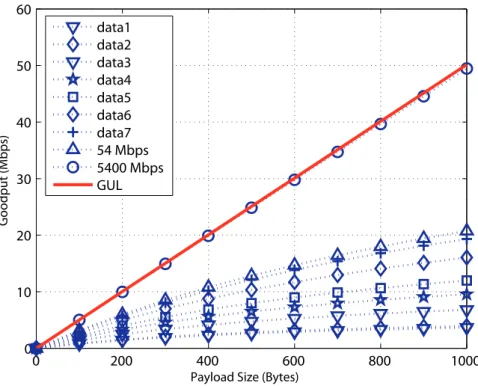
In [16–18], way to measure the performance of IEEE 802.11 MAC protocols in saturated throughput is proposed with similar method. In these works, a two-dimensional Makov chain model is used to model the backoff mechanism of distributed coordination function. Utilizing this model and channel access scheme e.g. RTS/CTS handshakes, the saturated throughput can be evaluated through a numerical method. With this method, the effect of increasing packet transmission rate (so-called data rate) on improving throughput is able to be estimated. But it is found that though the data rate can be increased to a extremely high value in use

0 200 400 600 800 1000 0 10 20 30 40 50 60

Payload Size (Bytes)

Goo dput (M bps ) data1 data2 data3 data4 data5 data6 data7 54 Mbps 5400 Mbps GUL

Figure 2.1: Theoretical goodput upper limit GUL in IEEE 802.11a protocols ignoring the channel noise.

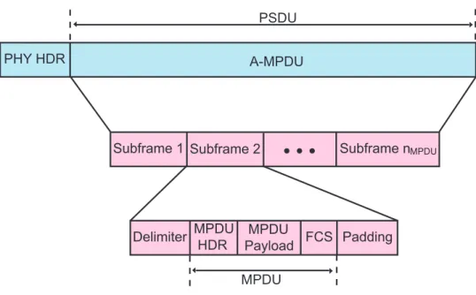
of these techniques, there is still a theoretical goodput uppper limit exist for IEEE 802.11 protocols. In the work of [7], it shows the existence of a theoretical goodput upper limit due to simply increasing the data rate without reducing the MAC/PHY overhead. In Fig. 2.1, it is shown that the enhanced performance in goodput bounded even when the data rates goes to infinitely high. Thus, mechanisms of frame aggregation and block acknowledgement are used for high-throughput IEEE 802.11 protocols. In IEEE 802.11n MAC layer protocols, two different frame aggregation formats are provided to improve the goodput. These two formats are aggregated MAC protocol data unit (A-MPDU) and aggregated MAC service data unit (A-MSDU) respectively. From the A-MPDU aggregation format shown in Fig. 2.2, it is easy to understand that an A-MPDU frame is the aggregation of nM P DU sub-frames.

Each sub-fame in an A-MPDU frame consists of a delimiter, a padding, and a single MPDU before aggregation, noting that the delimiter here is used as a partition of two consecutive MPDUs when doing the aggregation or de-aggregation operation. Referring to the MPDU,

PHY HDR

Subframe 1 Subframe 2 Subframe nMPDU

Delimiter MPDU HDR MPDU Payload FCS Padding A-MPDU PSDU MPDU

Figure 2.2: The frame format of A-MPDU.

a MPDU payload is passed down from the upper data link layer (DLL), and packaged with a MPDU header and a frame check sequence (FCS). Then the A-MPDU is passed down to PHY layer as the physical service data unit (PSDU) and packaged with PHY header. On the other hand, the A-MSDU aggregation format is shown in Fig. 2.3. Being different from the A-MPDU format, a single MPDU instead of an aggregation of few MPDUs is passed down to PHY layer to be a PSDU. In this single MPDU, an aggregation of nM SDU sub-frames is

taken as the payload, then packaged with MAC header and FCS. Similarly, each sub-frame in the A-MSDU consists of a MSDU which is separated from other MSDUs by a sub-frame header and a padding. With these two aggregation formats, the MAC/PHY overheads can be largely reduced in comparison with simply transmitting several un-aggregated MPDUs consecutively.

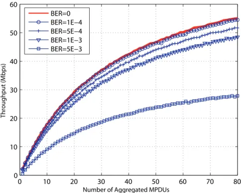
With these two aggregation formats introduced, performances versus different number of aggregation are evaluated in [19] to be compared. Based on the performances with different aggregated MPDUs and MSDUs shown in Fig. 2.4 and Fig. 2.5 from [19], it is found that an optimal aggregation number leads to maximum throughput exist only for the A-MPDU

PHY HDR

Subframe 1 Subframe 2 Subframe nMSDU

Subframe HDR MSDU MAC HDR FCS Padding A-MSDU PSDU

Figure 2.3: The frame format of A-MSDU.

formats. Referring to A-MSDU format, several sub-frames (MSDUs) are aggregated and packaged with a MAC header and one set of FCS. No matter how large the number of MSDUs aggregated is, there is only one set of FCS for error correction. And it means that as long as an uncorrectable error happened, information of all nM SDU sub-frames will be dropped.

Thus, if the number of aggregated number of MSDUs exceeds a certain limit, the efficiency of transmitting an A-MSDU frame will contrarily decrease. So that an optimal number of aggregated MSDUs leading to a peak value of throughput existing for A-MSDU format. Oppositely in A-MPDU format, every MPDU has already carried with its own FCS set before being aggregated. This means that all MPDUs are transmitted together, but they can be received independently because of separate FCS sets. Therefore, if a MPDU is received with uncorrectable error, only the information of this MPDU will be dropped. As a result, the throughput will increase as the number of aggregated MPDUs increases, and no optimal number leading to a peak value existing for A-MPDU format. And these two characteristics will be used later in the proposed FALA algorithm.

Assuming that A-MPDU format is used, the way of acknowledgement must be modified to record whether each MPDU is received successfully or not, i.e. the block

acknowledge-0 10 20 30 40 50 60 70 80 0 10 20 30 40 50 60

Number of Aggregated MPDUs

Throughpu t (Mb ps ) BER=0 BER=1E−4 BER=5E−4 BER=1E−3 BER=5E−3

Figure 2.4: Throughput of A-MPDU with different aggregation numbers.

0 10 20 30 40 50 60 70 80 0 5 10 15 20 25 30 35

Number of Aggregated MSDUs

Th roughput (Mbps ) BER=0 BER=1E−5 BER=2E−5 BER=5E−5 BER=1E−4

1st transmission attempt

bitmap in received BA for 1st transmission attempt

1 2 3 4 5 6 7 8 3 6 8 10 11 12 13 14 1 2 3 4 5 6 7 8 2nd transmission attempt Tr a nsmitter Receiver

Figure 2.6: Block Acknowledgement with Selective Repeat.

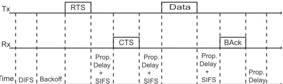
ment (BA). In a BA packet, a bit map is carried denoting which MPDU is received success-fully and which one is not. Another feature in BA is that a retransmission mechanism of selective repeat (SR) is used. With SR mechanism, any MPDUs failure will be retransmitted in the next transmission attempt, and unconcerned with the order in the A-MPDU. An exam-ple of MPDU retransmission with BA and SR is illustrated in Fig. 2.6 with eight MPDUs aggregated. As shown in figure, blocks with different numbers represent different MPDUs transmitted in a transmission attempt. The status of MPDU receiving is shown in the bitmap to each transmission attempt. Through checking the bitmap in a BA, a MPDU is considered received with uncorrectable error is marked as a block with cross on it, and the number of this block correspond to the MPDU needed to be retransmitted in the next transmission attempt. For example, MPDUs of number three and six in the first transmission are acked with uncor-rectable error, then these two MPDU will be transmitted in the second transmission attempt. At the end of this section, the CSMA/CA based RTS/CTS handshake scheme used in this work is shown in Fig. 2.7.

DIFS Backoff RTS Prop. Delay + SIFS CTS Prop. Delay + SIFS Data Prop. Delay + SIFS Prop. Delay BAck Time Tx Rx

Figure 2.7: The schematic diagram of RTS/CTS handshake operation.

2.2 Existing Link Adaptation Algorithms

In this section, two different categories of link adaptation algorithms will be introduced. In the ARF algorithm first proposed in [11], some simple rate-decision criterions are set, and only some parameters in MAC layer such as successful or failed transmission attempts are used. Being different from ARF algorithm, algorithms proposed in [12–14] took use of information estimated in PHY layer e.g. SNR on criterions of rate decision. And these two different types of link adaptation algorithm will be introduced as follows.

2.2.1 Automatic Rate Fallback (ARF) Algorithm

Referring to ARF algorithm proposed in [11], only some simple criterion added for MAC layer protocols, no significant modification of the MAC structure or complicated computa-tion is needed to implement it. The algorithm of ARF can be realized in Algorithm 1. As shown in Algorithm 1, counters nsucc/nf ail are set to trace consecutive successful/failed

transmission attempts, and a flag of f set is set to check the success of the first transmission attempt after data rate upgraded. As long as a consecutive successful transmission number of ten is reached, the data rate will be upgraded to a higher level and the flag of f set will be raised for the next transmission attempt. And if the next transmission is successful, this station will keep transmitting in this rate. But if the first attempt is unfortunately failed after rate-upgrading or a consecutive failure number of two reached, data rate will be reduced to a

Algorithm 1: Automatic Rate Fallback (ARF)

nsucc = 0 : initial number of consecutive successful transmission attempts ;

nf ail = 0 : initial number of consecutive failed transmission attempts ;

of f set : a flag to check if the first transmission attempt after the data rate level

upgrades is successful ;

while the queue of data packet is not empty do if a frame is acked successfully then

nsucc+ + ;

nf ail = 0 ;

if of f set = 1 then

of f set = 0 ;

if nsucc = 10 then

(adapt data rate to a higher level) ;

nsucc = 0 ; nf ail = 0 ; of f set = 1 ; else nsucc = 0 ; nf ail+ + ;

if nf ail = 2 or of f set = 1 then

(adapt data rate to a lower level) ;

nsucc = 0 ;

nf ail = 0 ;

lower level. These counters nsucc, nf ail and flag of f set will be traced as long as the packet

queue is not empty. However, without tracing the direct information of channel condition, criterion of rate decision in ARF algorithm is not precise enough and less sensitive to channel variation.

2.2.2 MAC and PHY Cross-Layer Link Adaptation (CLA) Algorithm

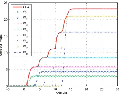
Due to the poor adaptability to channel variation of ARF algorithm, some similar link adap-tation algorithms utilizing the cross-layer information are proposed [12–14] to mitigate this drawback. For the convenience, this kind of algorithm is simply denoted as CLA algorithm. The saturated goodput analysis of IEEE 802.11 DCF is done and utilized in the rate-decision criterion of CLA algorithm. From the realization of CLA algorithm shown in Algorithm 2, an optimal MCS including modulation mode and coding rate will be chosen corresponding to a given SNR at the run time of the station. And the assignment of the optimal MCS is go-ing through a simple table mappgo-ing, and no computation needed at run time. The table used in CLA algorithm is established on the criterion of goodput maximization before the station starts to communicate. Noting that the saturated goodput is analyzed for DCF and IEEE 802.11a PHY protocols. There are eight MCSs provided in the standard of IEEE 802.11a [1]. The goodput with a single MCS used will vary from SNR estimated at the receiver end. Com-paring the performances utilizing every single MCS shown in Fig. 2.8, a trade-off between reliable transmission in low SNR and large goodput in high SNR can be found. With this phenomenon, the criterion of goodput maximization is used in CLA algorithm. For a given SNR, the most appropriate MCS is obtained through exhausted searching of goodput with all eight MCS used for the maximal one. Utilizing CLA algorithm leads to performance which is better than any other single mode. 2.

Since all the operation and the mapping table is preestablished, no more computations and evaluations are needed at the system run time. Thus the spare delay time caused by

−5 0 5 10 15 20 25 30 0 5 10 15 20 25 SNR (dB) Goodpu t ( Mbps ) CLA m 1 m 2 m 3 m 4 m 5 m 6 m 7 m 8

Figure 2.8: Goodput for single mode of eight different MCSs and CLA algorithm. Payload size is 2000 bytes.

Algorithm 2: Cross-layer Link Adaptation (CLA)

(compute the optimal MCS m∗_{(s, n) for n and given channel condition s) ;}

succ count = 0 : counter for successful transmission ; f ail count = 0 : counter for failed transmission ; F : the frame at the header of the data queue ; ncurr = 1 : counter for retransmission ;

while the queue of data packet is not empty do

scurr = the current wireless channel condition ;

mcurr = m∗(scurr, ncurr) ;

(F is transmitted using PHY mode mncurr) ;

if a frame is acked succesfully then

ncurr = 1 ;

succ count + + ;

else

ncurr+ + ;

if ncurr > nmaxthen

ncurr = 1 ;

f ail count + + ;

if ncurr = 1 then

(remove the header frame form the data queue) ; (refresh F ) ;

CLA algorithm is small than ARF algorithm. It means that the link can be adapted ”on time”, and the performance under serious channel variation will be largely improved. Also, the CLA algorithm will outperforms ARF algorithm in goodput because of the criterion of goodput maximization. After going through these two algorithms ARF and CLA, it is easy to find out that both MAC and PHY layer information are necessary to make the adaptation more accurate. And all efforts for link-adaptation criterion must be preestablished to make the adaptation on time. Moreover, any tunable parameters can be searched and taken into elements of the link-adaptation criterion to make the goodput as high as possible. Thus, in the proposed algorithm of this thesis, the payload size of a MPDU in A-MPDU format will be taken into consideration. And the parameter set of optimal MCS and MPDU payload size will preestablished into a table on the criterion of maximal goodput. Then the parameter sets will be the mapping table from a given SNR to optimal MCS and MPDU payload size and maximal goodput. These will be introduced in detail later in the next chapter.

Chapter 3

Proposed Frame-Aggregated Link

Adaptation (FALA) Algorithm

In this chapter, the saturation network goodput analysis with frame aggregation will be in-troduced in the section of ”Goodput Analysis for Frame Aggregation” with the MAC-layer BER evaluated before the saturation goodput. And the proposed FALA Algorithm will be introduced in detail in the section of ”Detail Description of Proposed FALA Algorithm”.

3.1 Goodput Analysis for Frame Aggregation

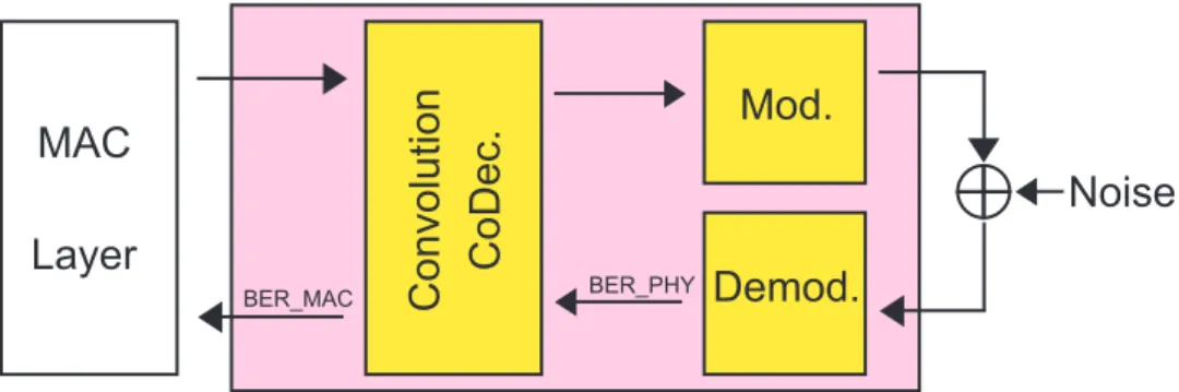
Considering a simplified transceiver block diagram with the modulation/demodulation and convolution coding/decoding blocks in IEEE 802.11 PHY layer protocols shown in Fig. 3.1, there are two types of BER observed from different points of view. One is the PHY layer BER caused by the demodulation error of signals transmitted under error prone channel, and the other one is the MAC layer BER including the additional decoding error of the codec block.

Noise

Convolution

Mod.

Demod.

CoDec.

MAC

Layer

BER_PHY BER_MAC

Figure 3.1: Mod./Demod. and Convolution coding blocks in PHY Layer.

PHY layer Pbe(mn) is needed. Only the demodulation block is considered when evaluating

Pbe(mn), so that the coding rate Rcis not not the necessary information. Considering MCSs

in Table 2.1, three different modulation modes (BPSK, QPSK, M-ary QAM) are utilized. For BPSK and QPSK with code rate Rc=1/2, and 3/4 (mn = 1, 2, 3, 4). Pbe(mn) is given

by (3.1) with SNR estimated at the receiver Eb/N0[20]. Q(x) is the complementary Gaussian

cdf. Pbe(mn) = Q( r 2Eb N0 ) , (3.1)

For 16-QAM with code rate Rc=1/2, 3/4, and 64-QAM with code rate Rc=2/3, 3/4 (mn=5,

6, 7, 8). Pbe(mn) is given by (3.2) with SNR estimated at the receiver Eb/N0 [20].

Pbe(mn) = 2(√M − 1) √ M log₂√MQ( s 2 log₂M · Eb N0 M − 1 ) + 2(√M − 2) √ M log₂√MQ( s 3 log₂M · Eb N0 M − 1 ) , (3.2) As mentioned before, the data are encoded using the convolutional encoder defined in IEEE 802.11a standard [1]. According to the convolutional encoder defined in [1], generator polynomials, g0 = (133)8 and g1 = (171)8, and constrain length K=7 are used.

With the generator polynomials and constrain length, the union bound of decoding-error probability Pde(mn) of rate Rc=1/2 and Rc=2/3, 3/4 (high rate through puncturing the

rate-1/2 code) are given by (3.3) [9], (3.4) and (3.5) [10] respectively. Pd(mn) is The probability

that an incorrect path selected with the Hamming distance d when doing the FEC decoding.

Pde(mn) < 11P10(mn) + 38P12(mn) + 193P14(mn) + ... , (3.3)

Pde(mn) < P6(mn) + 16P7(mn) + 48P8(mn) + ... , (3.4)

Pde(mn) < 8P5(mn) + 31P6(mn) + 160P7(mn) + ... , (3.5)

It’s assumed that the convolution forward error correcting (FEC) code is decoded with Viterbi decoding using hard decision. The probability of an incorrect path selected of Ham-ming distance d being even and odd are given by (3.6) and (3.7) respectively.

Pd(mn) = 1 2C d d/2Pbe(mn)d/2(1 − Pbe(mn))d/2+ d X k=d/2+1 Cd kPbe(mn)k(1 − Pbe(mn))d−k , (3.6) Pd(mn) = d X (d+1)/2 C_kdPbe(mn)k(1 − Pbe(mn))d−k , (3.7)

The convolution encoder used here encodes each bit from MAC layer into 2 symbol with 7 bits, i.e. 14 bits totally. The average BER in MAC layer Pe(mn) is derived from taking

the first 3 terms of the union bound of Pde(mn) in (3.3) to (3.5) as the approximation of

Pde(mn) first, then dividing the approximative Pde(mn) by 14. The diagrams of average

BER in PHY layer Pbe(mn) versus SNR Eb/N0 and average BER in MAC layer Pe(mn)

−5 0 5 10 15 20 25 10−7 10−6 10−5 10−4 10−3 10−2 10−1 100 E b / N0 (dB) BER m 1,m2 m 3,m4 m 5,m6 m 7,m8

Figure 3.2: The average PHY-layer BER corresponding to given mnis denoted as Pbe(mn).

−5 0 5 10 15 20 10−7 10−6 10−5 10−4 10−3 10−2 10−1 100 E b / N0 (dB) m 1,m3 m 2,m4 m 5 m 6 m 7 m 8

After the evaluation of MAC-layer BER Pe(mn) from SNR estimated at receiver end. The

saturated goodput of the network can be analyzed under a two-dimensional Markov chain backoff model shown in Fig. 3.4. Referring to the backoff model in Fig. 3.4, every backoff operation (s(t), b(t)) consists of two stochastic processes s(t)∈[0, m] and b(t)∈[0, Wi − 1].

In a backoff operation, the process s(t) indicates the backoff stage with the maximum stage

m which is the system retry limit, and the process b(t) denotes the backoff timer at each ith

backoff stage with value of ithcontention window size Wi represented as follow.

Wi = 2i·W 0≤i≤m (3.8)

From (3.8), it can be found that the minimum size (CWmin) and maximum size (CWmax) of

the contention window are denoted as W0and Wmrespectively. With the assumption of nST A

stations exist to contend the access right of channel, a random state from (0, 0) to (0, W0− 1)

will be chosen to back off since a station starts to transmit. When any station counts to state (0, 0), it tries to transmit an A-MPDU frame. The backoff operation will jump to the next backoff stage if the transmission of this A-MPDU is failed, and similarly a random state from (1, 0) to (1, W1− 1) is chosen to back off. And if the transmission at the mth stage failed,

the whole A-MPDU will be dropped and the operation will be reset to any state in the initial 0th stage. Oppositely, if a successful transmission happened in any ith backoff stage, the

operation will be reset to any state in the initial 0thstage.

To derive the stationary distribution of the backoff model in Fig. 3.4, the state-transition probability should be evaluated first. Assuming that the stage changes with a successful transmission or failed transmission due to collision and noise interference. Denoting the stage-transition probability when the backoff timer expires as p. Then, the state-transition probabilities defined as P (i1, k1|i0, k0),(s(t + 1) = i1, b(t + 1) = k1|s(t) = i0, k(t) = k0)

0,0 0,1 0,2 0,W0-1

i

_-1,0

i

_,0

i

_,1

i

_,2

i

_{,Wi -1} m,0 m,1 m,2 m,Wm-1 (1-p)/W0 p/W1 p/Wi p/Wi ₊₁ p/Wm 1 1 1 1 1 1 1 1 1 1 1 1 (1-p)/W0 (1-p)/W0 1/W0

Figure 3.4: Two-dimensional Markov chain backoff model in consideration of packet colli-sion and noisy channel for DCF function.

can be obtained as follows:                  P (i, k|i, k + 1) = 1 k ∈ [0, Wi− 2], i ∈ [0, m] P (i, k|i − 1, 0) = _Wp i k ∈ [0, Wi− 1], i ∈ [1, m] P (0, k|i, 0) = 1−p_W0 k ∈ [0, W0− 1], i ∈ [0, m − 1] P (0, k|m, 0) = 1 W0 k ∈ [0, W0− 1] (3.9)

With the state-transition probabilities assumed, the stationary distribution defined as πi,k ,

limt→0P (s(t) = i, b(t) = k) with i ∈ [0, m], k ∈ [0, Wi− 1] can be derived as follows:

           πi,0 = πi−1,0· P_Wi−1 k=0 Wpi = πi−1,0· p i ∈ [1, m] πi,k = πi−1,0· P_Wi−1 j=k Wpi = πi−1,0· p · Wi−k Wi i ∈ [1, m], k ∈ [0, Wi− 1] π0,k = W_W0−k₀ · (1 − p) · P_m−1 j=0 πj,0+WW0−k0 · πm,0 k ∈ [0, W0− 1] (3.10)

Then, (3.11) expresses the stationary distribution πi,k, ∀i, k of (3.10) in terms of π0,0.

     πi,0= pi· π0,0 i ∈ [1, m] πi,k = W_Wi−k_i · πi,0 i ∈ [0, m], k ∈ [0, Wi− 1] (3.11)

The characteristics of the Markov chain model can be illustrated in (3.11) with probability p. And the following is the determination of the p.

Utilizing the backoff model in Fig. 3.4, the probability that any transmission happened within a randomly selected time slot, i.e. the conditional transmission probability τ , can be expressed in (3.12). τ = m X i=0 πi,0 = π0,0· m X i=0 pi = π0,0· 1 − p m+1 1 − p (3.12) The characteristics of the two-dimensional Markov chain model can be illustrated via (3.9)-(3.15) after the stage-transition probability p can be obtained. The determination of p is

explained as follows:

p = Pcollision+ (1 − Pcollision)Pf e,A−M P DU(mn, l) (3.13)

In (3.13), Pcollision denotes the collision probability and the error probability of the whole

A-MPDU with MCS mn, payload size l chosen is denoted as Pf e,A−M P DU(mn, l). And

Pcollissionand Pf e,A−M P DU(mn, l) can be expressed as

     Pcollision= 1 − (1 − τ )nST A−1 Pf e,A−M P DU(mn, l) = Pf e,M P DU(mn, l)nM P DU (3.14)

where nST A and Pf e,M P DU denote the total number contend to access the channel and the

frame error rate (FER) of a single MPDU in noisy channel. Another point to note is that the effect of noises on p is Pf e,A−M P DU, which means any transmission attempt will be taken as

failure only if every MPDU in an A-MPDU is received with uncorrectable error. It is obvious that the stage-transition probability p can be expressed as the function of the conditional transmission probability τ . Therefore, expressing τ in terms of p, then the values of p can be acquired through numerically solving the nonlinear equations of (3.12) and (3.13).

Consequently, express πi,k, ∀i, k in terms of π0,0 via (3.11). The state probability π0,0

can be obtained by normalizing the stationary cumulated distribution of Markov chain model to one, i.e. Pm_i=0PWi−1

0

_,0 1

0

_,1 1

0

_,2 1

0

_,W0-1 1

0

_,W0-2 1 1/W0

Figure 3.5: One-dimensional, simplified backoff model when stage-transition probability p in Fig. 3.4 is nearly zero.

shown in (3.15). 1 = Pm_i=0PWi−1 k=0 πi,k = π0,0· P_m i=0 P_Wi−1 k=0 pi· WWi−ki ⇒ π0,0 = [ P_m i=0 P_Wi−1 k=0 pi· WWi−ki ] −1 = _(1−pm+1_)(1−2p)2(1−p)(1−2p)_{+ W (1−p)[1−(2p)}m+1_] (3.15)

Then a numerical solution of p can be evaluated through iteratively solving (3.12), (3.13) with parameters of m, mn, nST A, nM P DU, l assigned and a given SNR. Noting that if the solution

of p is nearly zero, the backoff model can be simplified to an one-dimensional Markvo model as shown in Fig. 3.5. And the conditional transmission probability can be acquired through the same procedure of stationary distribution normalization.

τ = π0,0 = [ PW0−1 k=0 WW0−k0 ] −1 = 2 W +1 (3.16)

This can reduce the computation later when evaluating the value of saturated network good-put.

With the solutions obtained and considering the RTS/CTS access scheme shown in Fig. 2.7 utilized, the saturated network goodput can ba evaluated as follows. Being similar to works presented in [16–18] and frame aggregation mechanism added, the saturated goodput

expressed in (3.17) can be defined as the fraction of average information earned of an A-MPDU, and the time needed to successfully transmit an A-MPDU. Noting that a successfully transmitted A-MPDU requires at leat one MPDU in it is received with correctable error.

G(l, mn) =

E[P ayload] E[Tpayload]

= E[P ayload]

E[TB] + E[TS] + E[TC] + E[TE]

(3.17)

In order to emphasize the impact of different parameter set chosen in the proposed FALA algorithm, the saturated goodput in (3.17) is denoted as a function of payload size of a single MPDU, l, and MCS, mn. And with the following evaluations will the saturated goodput

obtained. First of all, two important probabilities Ptr and Pwc will be introduced. Ptr in

(3.18) is the probability that at least one transmission occurring in the considered time slot, i.e. at least one station is transmitting.

Ptr = 1 − (1 − τ )nST A (3.18)

Pwcin (3.19) is the probability of transmission without collisions on condition that at leat one

station is transmitting. Pwc= nST A· τ · (1 − τ )nST A−1 Ptr = nST A· τ · (1 − τ )nST A−1 1 − (1 − τ )nST A (3.19)

In (3.17), E[TB] = (1 − Ptr) · σ indicates the average length of the non-frozen backoff time

in a time slot, where σ is defined as the size of a slot time [16]. The average duration of the successful transmission in a time slot and mean length of a failure transmission caused by channel noises are denoted as E[TS] and E[TE] respectively. Furthermore, E[TC] represents

E[TC] are obtained in the following equations.

E[TS] = Ptr· Pwc· [1 − Pf e,A−M P DU(mn, l)] · TSuccess (3.20)

E[TE] = Ptr· Pwc· Pf e,A−M P DU(mn, l) · TError (3.21)

E[TC] = Ptr· (1 − Pwc) · TCollision (3.22)

In (3.20) and (3.21), TSuccess and TError are time intervals required for a successful or failure

transmission of an A-MPDU respectively. According to the RTS/CTS scheme illustrated in Fig. 2.7, the TSuccess = TErrorcan be expressed as

TSuccess = TRT S+ TCT S+ THeader+ TP ayload+ TBlockAck+ 3TSIF S+ 4ρ + TDIF S (3.23)

which consists of the transmitting time of an A-MPDU frame and the MAC/PHY overheads needed to transmit it, where the note ρ represents the propagation delay. moreover, Tcollision

is time wasted if a collision case shown in Fig. 2.7 happened.

TCollsion = TRT S+ ρ + TDIF S (3.24)

Finally, the term E[P ayload] in (3.17) is the average information received successfully from payload of each MPDU transmitted in a time slot. It can be acquired as

E[P ayload] =PnM P DU

i=0 CinM P DU · (1 − Pf e,M P DU(mn, l))i· Pf e,M P DU(mn, l)nM P DU−i· i · l

= nM P DU · l

where the dummy variable i denotes the number of successful received MPDUs in a A-MPDU transmission attempt. Then the saturated goodput G(l, mn) with MPDU-payload size l and

MCS mnis acquired through substituting (3.18) - (3.25) into (3.17).

3.2 Detail Description of Proposed FALA Algorithm

In this section, the system architecture, principles, and implementation in pseudo code of the proposed FALA algorithm in this work will be introduced in detail as follows. First, considering the CLA algorithm [12], the maximal goodput with a given SNR is searched from goodput with all possible MCSs applied. The payload size of a single MPDU is set to a fixed number. Then reminding the feature of optimal frame size found in [19], the same feature is existed for payload size of a single MPDU in A-MPDU format. An example with MCS m2applied is taken to realize this feature, and the payload size ranges from ten to eight

thousand bytes to search for the optimal payload size. As shown in Fig. 3.6, a system in operation of m2 with optimal payload size can obtain the highest goodput than any other

system with only fixed payload size available. Secondly in Fig. 3.7, it is obviously that with m2 applied, the optimal payload size of MPDU is different for different given SNR.

Thus, the MPDU payload size is a possible term to maximize the goodput. So it is worthy of preestablishing a table with optimal parameter set of mnand l to maximize the performance

over different channel condition. This is the main idea of the proposed FALA algorithm. Before going through the detailed algorithm, the concept of the proposed FALA algorithm can be realized through a simple cross-layer system architecture for MAC and PHY layer protocols shown in Fig. 3.8. In Fig. 3.8, the MAC and PHY layer protocols of IEEE 802.11 standard is not modified. Only an extra block of FALA algorithm is added to act as the link adaptor. Referring to the FALA algorithm block, the SNR estimated at the received end is fed into the BER Evaluator to evaluate the MAC-layer BER. Then the MAC-layer BER extracted

−5 0 5 10 15 20 25 30 0 2 4 6 8 10 12 14 16 18 E b / N0 (dB) Goodput (Mbps ) Opt l* 10 100 500 1 K 5 K

Figure 3.6: Goodputs with m2 applied in cases of the MPDU payload size l = l∗, l > l∗_{, andl < l}∗_.

in the BER Evaluator is sent to find out the corresponding parameter set (m∗

n, l∗) in the block

of FALA Table. The corresponding (m∗

n, l∗) will be passed to MAC-layer to adapt the link

of next transmission attempt. Through the realization of the system architecture in Fig. 3.8, it is easy to find that the FALA Table is the kernel of FALA algorithm and most work of this algorithm is the establishment of this table. The flow to establish the FALA Table is described in Table 3.1. As shown in Table 3.1, the first step to establish the FALA Table is collecting some necessary system information, e.g. A-MPDU aggregation number nM P DU, all MCSs

(mn) provided and available payload sizes l ranges from lmin to lmax stepped by lscale. Then

deciding the concerned SNR ranges from SN Rmin to SNRmax stepped by SNRscale, and

note that the FALA Table is more accurate with larger SNR range. With these parameters set, the saturated goodput introduced at last section can be evaluated through any possible numerical solutions. With goodput corresponds to all given parameters evaluated, the desired

b 0 −5 0 5 10 15 20 25 30 0 20 Max imal Goodput of m 4 E / N (dB) −5 0 5 10 15 20 25 300 1 2 3 4 5 6 7 8 9 10 Optimal Pa y load Size (K By tes) of m 4 Payload size Goodput

Figure 3.7: Maximum goodput and optimal MPDU payload size of mn with the optimal

payload size used.

Note : The FALA Table is established before the system starts to transmit. Step I : Collecting the information of system parameters

(1) Evaluate the MAC BER Pe(mn) ∀ MCS (mn) available

(2) ∀ payload size (l) available stepped by scale l_scale Step II : Setting the concerned range of SNR

SNR ∈ [SN R_min, SN R_max] stepped by SN R_scale Step III : Calculations of saturated goodput

evaluate G(m_n, l) for ∀m_n, l with a given SNR Step IV : Elements of FALA Table obtained.

(m∗

n, l∗) with a given SNR is obtained through exhausted search.

Wireless Channel

Data Link Layer

MAC Layer

PLCP

OFDM

SNR

Estimator

(SNRi)

MCS & Payload Size Selector FALA Table of (mn*,l*)

Ph

ys

ic

al

La

y

er

FALA

MSDU A-MPDU G*(mn*,l*) (mn*,l*)

Figure 3.8: The system architecture for MAC and PHY protocols with the proposed FALA algorithm implemented.

optimal link adapting parameter set (m∗

n, l∗) and maximal goodput are then obtained and

based on the criterion expressed in (3.26). (m∗

n, l∗) = arg max∀mn,∀lG(mn, l) G∗_(m

n, l) = G(m∗n, l∗), with given SNR

(3.26)

Noting that when implementing FALA algorithm, the SNR axis is divided into nSN R

sec-tions, and the estimated SNR located in the same section will leads to the same (m∗

n, l∗) and

G∗_(m

n, l). This is illustrated in Fig. 3.9 and the format of corresponding FALA Table is

shown in Table 3.2. Where the term nSN R which can be expressed as in (3.27) represents s

the number of SNR values used to evaluated MAC BER for goodput evaluations.

nSN R =

SNRmax− SNRmin

SNRscale

SNRmin + SNRscale (mn*,l*)2 SNRmin (mn*,l*)1 SNRmin + 2*SNRscale (mn*,l*)3 SNRmax -SNRscale (mn*,l*)nSNR-1 SNRmax (mn*,l*)nSNR SNR

SNRscale SNRscale₂ SNRscale₂

Figure 3.9: The SNR axis is bounded by SNRmin and SNRmax, divided by SNRscale into

nSN R regions.

The FALA Table

1st 2nd . . . . (nSN R− 1)th nSN Rth

region region region region

(m∗

n, l∗)1 (m∗n, l∗)2 . . . . (mn∗, l∗)nSN R−1 (m∗n, l∗)nSN R

Table 3.2: The FALA Table in FALA algorithm.

With the system architecture realized and the FALA Table established, the pseudo code of FALA algorithm is shown in Algorithm 3. As shown in Algorithm 3, the original transmit-ting and receiving mechanisms of MAC protocols are kept unchanged. The additional effort done in system run time is to keep tracing the channel conditions, then deciding the optimal MCS and MPDU payload size for the next wireless link. As mentioned before, there is surely no additional calculation needed to be done at system run time.

Algorithm 3: Proposed Frame-Aggregated Link Adaptation Algorithm (m∗

n, l∗) set preestablished ;

lt: the MPDU payload size in current transmission attempt of an A-MPDU ;

mnt = m1: the initial value of MCS in current transmission ; m = 7: the retry limit ;

while queue of data packet is not empty do

count successt= 0 ;

count f ailt= 0 ;

nt = 0, the count of transmission attempts;

SNRt: the channel condition in current transmission attempt ;

mnt=m

∗

n lt= l∗ correspond to SNRt;

(the first nMP DU frames at the head of the queue of data are transmitted) ;

if an A-MPDU packet received then

if a subframe the A-MPDU received with no error then

count successt= count successt+ 1 ;

else

count f ailt= count f ailt+ 1 ;

(check the all nM P DU subfrmaes in the A-MPDU, and remove the

count successtsuccessfully transmitted subframe in the queue of data) ;

if count successt= 0 then

nt = nt+ 1 ;

count successt= 0 ;

count f ailt= 0 ;

else

nt = nt+ 1 ;

(this means the total nM P DU subframes are received with error);

count successt= 0; count f ailt= 0 ; if nt> m then nt = 0 ; count successt= 0 ; count f ailt= 0 ;

Chapter 4

Performance Evaluation

In this chapter, the performance in saturated goodput of single mode operation, and system with CLA [12] and the proposed FALA algorithm applied respectively from numerical anal-ysis will be compared in section of Analytical Results. Moreover, an example going through the implementation of FALA algorithm will also be demonstrated. Then the performance of three kinds of link adaptation algorithms will be compared in average saturated goodput and adaptability under time varying channel.

4.1 Analytical Results

First of all, an example will be demonstrated to show the flow of the evaluation of MAC-layer BER, goodput and establishment of FALA Table. Then the maximal goodput and optimal (m∗

n, l∗) will be found out and taken to implement FALA algorithm in simulations. The first

thing of FALA Table establishment is to collect the system information. Here as an example, the A-MPDU aggregation number nM P DU is assigned to be sixty four. The payload size of

single MPDU ranges from ten to fifty bytes stepped by ten bytes, and the SNR is bounded in [SNRmin = −5dB, SNRmax = 30dB] stepped by 0.5dB. With the method shown in

−5 0 5 10 15 20 25 30 0 10 20 30 40 50 60 E b / N0 (dB) Goo dput (Mbps ) FALA m 1 m₂ m 3 m₄ m 5 m 6 m₇ m 8

Figure 4.1: Goodput with FALA algorithm implmented and eight single MCSs. MAC-layer BER and goodput. These nST A = 71 regions can be listed as

SNRi = SNRmin+ (i − 1) · SNRscale i ∈ [1, nSN R]

SNRregion(i) ∈ [SNRi− SN R₂scale, SNRi+SN R₂scale) i ∈ [2, nSN R− 1]

SNRregion(1) ∈ (−∞, SNRmin+ SN R₂scale) i = 1

SNRregion(nSN R) ∈ [SNRmax− SN R₂scale, ∞) i = nSN R

(4.1)

where the note SNRi is the given SNR representing the region SNRregion(i), i.e. any SNR

value locates in region SNRregion(i) will be approximated as SNRi. The maximal goodput

shown in Fig. 4.1 is acquired through exhausted search based on the criterion of (3.26). Then the FALA Tabel is established with optima (m∗

n, l∗) corresponding to given SNR, and

is shown in Fig. 4.2. The simulation of FALA algorithm is based on the table established above. And the performance of systems applying FALA algorithm will be compared with others applying ARF and CLA algorithms in next section.

−5 0 15 20 25 30 0 1 2 3 4 5 6 7 8 Optimal MCS m n E b / N0 (dB) −5 1 4.5 7 9.5 11 15 20 25 0 1 2 3 4 5 6 7 8 Op tima l P ayload Size (K B ytes ) Optimal l* Optimal m n *

Figure 4.2: Optimal mn∗ and l∗based on FALA algorithm.

4.2 Simulation Results

4.2.1 Simulation Parameters

In this section, the simulation results are verified with the numerical results for error prone channel. The simulation models are constructed based on the parameters listed in Table 4.1. The MAC header includes the MPDU header, delimiter and the FCS in a subframe of A-MPDU. The PHY header includes the PLCP header and PLCP preamble transmitted in PLCP rate at 6 Mbps. The propagation delay and slot time are denoted as ρ and σ.

4.2.2 Model Validation

The searching and establishing of FALA Table from numerical analysis is already shown in Fig. 4.1 and the comparison of numerical and simulation results is shown in Fig. 4.3. In this comparison, the station number and A-MPDU aggregation number are nST A = 2 and

Parameters for Simulation

RTS 20 Bytes

CTS 14 Bytes

Block Ack 32 Bytes

MAC Header 24 Bytes

PHY Header 24 Bytes

SIFS 16 µs DIFS 34 µs Propagation Delay, ρ 1 µs Slot Time, σ 9 µs Retry Limit 7 CW_min 32 CW_max 4096

Table 4.1: MAC and PHY Defined Parameters

nM P DU = 64 respectively. And the MPDU payload size is searched from ten to five thousand

bytes stepped by ten bytes.

4.2.3 Performance Comparison

In this section, both of the performance in cross-layer goodput versus SNR, average goodput under time-varying channel and adaptability to channel variation with ARF, CLA, and FALA algorithms implemented willbe compared. First of all, comparison in goodput of FALA and CLA with MPDU payload size of five thousand bytes and sixty four MPDUs aggregated is shown in 4.4. And the different MCS assigned to be used corresponding to different given SNR is shown in Fig. 4.5. Obviously, CLA algorithm can perform as well as FALA algorithm do in goodput when channel condition is good enough. But a poor performance of CLA algorithm can be found in bad channel condition. It reveals the draw back of CLA algorithm in use of fixed MPDU payload size. This makes the CLA algorithm can not look after both sides of goodput in good/bad channel conditions. on the other hand, system with FALA algorithm will upgrade the data rate to transmit in higher rate earlierly when the one with CLA is still transmitting in low rate.

−5 0 5 10 15 20 25 30 0 10 20 30 40 50 60 E b / N0 (dB) Goodput (Mbps ) FALA (Anal) FALA (Sim) MCS (Anal) MCS (Sim)

Figure 4.3: Comparison of simulation and numerical results in the scenario of nST A = 2 and

nM P DU = 64. −5 0 5 10 15 20 25 30 0 10 20 30 40 50 60 E b / N0 (dB) Goodput (Mbps ) FALA CLA

Figure 4.4: Performance in goodput of FALA algorithm with payload size l ∈ [10, 5000] bytes available and CLA algorithm with payload size l = 5000 bytes.

−50 0 5 10 15 20 25 30 1 2 3 4 5 6 7 8 9 E_b/N₀ (dB) MCS (m n ) FALA CLA

Figure 4.5: Different decisions in MCS versus SNR of FALA and CLA algorithms.

good

bad

P

b,g

P

g,b

P

g,g

P

b,b

In order to compare the performance under different channel condition and adaptability to the channel variation. A two-state discrete Markov chain is introduced to model the channel variation. Considering the channel variation mode shown shown in Fig. 4.6, the channel is divided into two different conditions denoted as good and bad. In good channel condition, the SNR is uniform distributed from 10 dB to 25 dB, and in bad channel condition, the SNR is uniform distributed from -5 dB to 10 dB. The probability Pb,g, Pb,b, Pg,b, Pg,g means the

probability of channel varying between good and bad conditions or being unchanged in the same condition. For an example, a probability Pb,g = 0.7 means that channel condition will

probably varies from bad to good in 70%. And the channel model with larger Pb,g will stay

in good condition more often.

To show that the link adaptation algorithm designed with cross-layer information will have better than that with the MAC layer information only, a probability Pb,d = 0.7 is

as-signed. And it is assumed that channel variation will happen between different A-MPDU transmission attempts. In Fig. 4.7, two algorithms of FALA and ARF are compared, and a period of a hundred transmissions of A-MPDUs are taken to observe the MCS used in every attempt. In ARF algorithm, the MCS assigned for every attempts varies slowly because that ARF uses consecutive successful or failed transmission attempts to adapt the rate. Obviously ARF can not adapts the channel in high degree of variation. Other than ARF, the proposed FALA algorithm is much better in adapting the channel variation, and can adapt the link to optimal MCS as the channel varies.

Then comparison of average goodput between system with ARF, CLA and FALA al-gorithms implemented in different degrees of channel variation with Pb,g form zero to one

stepped by 0.1 is shown in Fig. 4.8. It is obviously to see that CLA outperforms ARF be-cause of its optimal m∗

nselection based on the criterion of goodput maximization. And FALA

outperforms CLA because that the every transmission in FALA utilizing not only the optimal

m∗

0 20 40 60 80 100 0 10 20 E b /N 0 (d B) 0 20 40 60 80 100 2 4 6 8 MCS (m n ) 0 20 40 60 80 100 2 4 6 8

Number of Transmitted A−MPDUs

MCS

(m

n

)

Figure 4.7: The first diagram is the channel conditions with in different transmission attempts generated by applying the two-state discrete Markov chain model with Pb,g = 0.7. The

second and the third one is PHY mode used in every transmission attempts of ARF and FALA respectively. 0 0.2 0.4 0.6 0.8 1 0 5 10 15 20 25 P_b,g Goo dpu t (Mbps ) FALA CLA ARF m 1 m 8

Figure 4.8: Average goodput of FALA , CLA and ARF under the varying channel with dif-ferent Pb,g from 0 to 1.

Average A-MPDU dropped rate

P_b,g m1 m8 ARF CLA FALA

0.0 0.097 1.000 0.202 0.071 0.043 0.1 0.084 0.930 0.198 0.067 0.041 0.2 0.081 0.864 0.177 0.064 0.041 0.3 0.079 0.793 0.175 0.055 0.038 0.4 0.071 0.726 0.173 0.051 0.038 0.5 0.070 0.680 0.171 0.048 0.036 0.6 0.052 0.568 0.170 0.041 0.035 0.7 0.050 0.499 0.164 0.040 0.035 0.8 0.049 0.484 0.154 0.036 0.034 0.9 0.048 0.399 0.151 0.034 0.031 1.0 0.048 0.337 0.138 0.033 0.030

Table 4.2: Average A-MPDU dropped rate.

Chapter 5

Conclusion

Because of the non-ideality of wireless nature, the channel condition can be good or bad in different environments. Transmitting with single MCS will not benefit in both good and bad channel conditions. Using a low-data-rate MCS is robust when in terrible channel conditions, but will cause low goodput when the channel condition is good enough for transmission in higher rates. Oppositely, using a MCS with high data rate will have large goodput when the channel condition is good enough, but may work terribly in bad channel condition due to transmission errors. Beside this, the channel condition may not always be stable, and may vary during any transmission period. Thus, a link adaptation algorithm is necessary not only in decision of optimal MCSs for different channel conditions but also in adaptation to the variation of channel conditions. As shown in performance comparison of simulation results, the proposed algorithm FALA outperforms the two typical algorithm compared in goodput, and has good adaptability against channel variation. Therefore, it is undoubtedly that the proposed FALA algorithm is a link adaptation algorithm with high goodput and adaptability to channel variation.

Bibliography

[1] IEEE 802.11 WG, ”IEEE Std 802.11a-1999(R2003): Part 11: Wireless LAN Medium Access Control (MAC) and Physical Layer (PHY) specifications: High-speed Physical Layer in the 5 GHz Band,” 2003.

[2] IEEE 802.11 WG, ”IEEE Std 802.11b-1999(R2003): Part 11: Wireless LAN Medium Access Control (MAC) and Physical Layer (PHY) specifications: Higher-Speed Physical Layer Extension in the 2.4 GHz Band,” 2003.

[3] IEEE 802.11 WG, ”IEEE Std 802.11g-2003: Part 11: Wireless LAN Medium Access Control (MAC) and Physical Layer (PHY) specifications: Amendment 4: Further Higher Data Rate Extension in the 2.4 GHz Band,” 2003.

[4] IEEE 802.11 WG, ”EEE Std 802.11e-2005: Part 11: Wireless LAN Medium Access Control (MAC) and Physical Layer (PHY) specifications: Amendment 8: Medium Ac-cess Control (MAC) Quality of Service Enhancements,” 2003.

[5] IEEE 802.11, ”HT PHY Specification V1.27,” Enhanced Wireless Consortium

publica-tion, Dec. 2005.

[6] IEEE 802.11, ”HT MAC Specification V1.24,” Enhanced Wireless Consortium

[7] Y. Xiao, and J. Rosdahl, ”Throughput and Delay Limits of IEEE 802.11,” IEEE Commun.

Lett., pp. 355-357, 2002.

[8] D. Tse, P. Viswanath, ”Fundamentals of Wireless Communication,” Cambridge

Univer-sity Press, 2005.

[9] J. Conan, ”The Weight Spectra of Some Short Low-rate Convolution Codes,,” IEEE

Transaction on Communications, Vol. 32, pp. 1050-1053, Sep. 1984.

[10] D. Haccoun and G. Begin, ”High-rate Punctured Convolution Codes for Viterbi and Sequential Decoding,”IEEE Transaction on Communications, Vol. 37, pp. 1113-1120, Nov. 1989.

[11] A. Kamerman, L. Monteban, ”WaveLAN-II: A High-performance Wireless LAN for the Unlicensed Band,” Bell Labs Technical Journal, pp. 118-133, Aug. 1997.

[12] D. Qiao, S. Choi, K. G. Shin, ”Goodput Analysis and Link Adaptation for IEEE 802.11a Wireless LANs,” IEEE Transactions on Mobile Computing, Vol. 1, pp. 278-292, 2002. [13] J. D. P. Pavon, S. Choi, ”Link Adaptation Strategy for IEEE 802.11 WLAN via Received

Signal Strength Measurement,” IEEE International Conference on Communications, Vol. 2, pp. 1108-1113, 2003.

[14] H. Nakase, S. Kameda, H. Oguma, K. Tsubouchi, ”A Closed-Loop Link Adaptation Scheme for 324Mbit/sec WLAN System,” IEEE International Symposium on Personal,

Indoor and Mobile Radio Communications, 2007.

[15] R. P. F. Hoefel, ”A MAC and PHY Cross-Layer Analytical Model for the Goodput for the Goodput and Delay of IEEE 802.11a Networks Operating Under Basic Access and RTS/CTS DCF Schemes,” Journal of Communications, Vol. 1, Sep. 2006.