AgvSimNet: A Petri net based AGVS simulation system

(1)

 1999 Springer-Verlag London Limited

AgvSimNet: A Petri-Net-Based AGVS Simulation System

S. Hsieh and Y.-F. Chen

Department of Mechanical Engineering, National Taiwan University, Taipei, Taiwan

This paper presents a Petri-net (PN) based automated guided vehicle system (AGVS) simulation system, AgvSimNet. The sys-tem is designed so that it can be used not only for off-line evaluation of a given flow-path layout and/or management strategy, but also for on-line system monitoring and dynamic dispatching control. AgvSimNet adopts modular PN modelling techniques for constructing complicated AGVS models. End-users of the system are not required to write any code to conduct their simulation tasks. Some special functions of the AGVS, such as zone control, blocking phenomenon and two-step-ahead forecast, are incorporated into the system. These special functions make the AGVSimNet model more accurate. Several common vehicle management rules are included in the system for users’ elaboration and comparative study. Two verification and three application examples are presented to show the effectiveness of AgvSimNet. The results indicate that AgvSimNet gives satisfactory results for AGVS off-line evalu-ation. It also opens a promising new direction in applying simulators for on-line AGVS monitoring and dynamic vehicle dispatching control.

Keywords: AGVS; Coloured-timed Petri nets; Off-line simul-ation; On-line monitoring

1. Introduction

Material handling is one of the most important functions that affects the efficiency of a manufacturing system. Automated guided vehicle systems (AGVSs) are widely used material-handling systems in modern manufacturing systems that possess some attractive characteristics including flexibility, efficiency and integration with other components in the system.

An automated guided vehicle (AGV) is an unmanned vehicle that transports loads from one location to another. The capabili-ties of an AGVS have been increased and are well suited for modern, automated facilities. With improvements such as

Correspondence and offprint requests to: S. Hsieh, Department of Mechanical Engineering, National Taiwan University, No. 1 Roosevelt Road, Sec. 4, Taipei, Taiwan 10764. E-mail: shhsieh얀w3.me. ntu.edu.tw

automatic loading and unloading, the ability to transport a wide variety of materials and the capability to interface with a range of other equipment, AGVSs are becoming a common method of material handling.

An AGVS is sensitive to many complex interactions that exist in the system and is also sensitive to the coordination of vehicles with the rest of the system. Many simulation models have been constructed in the past for the study of AGV systems. For example, models were built to analyse vehicle routeing [1], to plan and test flow-path layouts [2], and to study the potential for bi-directional flow [3]. In addition, Harmonosky and Sadowski [4] presented a SIMAN model to study the integration of AGVs with conventional material-handling equipment.

As an alternative to simulation, analytical approaches to the design of AGV systems have been proposed. For example, mathematical models have been used to estimate the required number of vehicles for a given system [5,6] and to design the flow-path layout [7,8]. However, mathematical techniques can produce baffling problems when applied to industrial cases. Moreover, these approaches have been shown to give inaccurate estimates under certain control strategies [9]. This is also true for queuing-based procedures, as these procedures fail to cap-ture the dynamic nacap-ture of an AGVS [10,11].

Matzener [12] pointed out the importance of system simul-ation and how to write an AGVS simulator. In industry, AGVS simulators have been developed in the past by using general-purpose simulation languages such as GPSS/H [13], SLAM and SIMAN [10], and AutoMod [12]. Matzener [12] pointed out that the results of simulation and the validity of perform-ance forecasting depend significantly on the skill and experi-ence of the simulation program developer. King and Kim [14], therefore, established an object-oriented AGVS simulator, AgvTalk. Gaskins and Tanchoco [1] built a package called AGVSim2 by using the general procedure language C. Araki et al. [15] developed a BASIC language based AGVS simulator that allows flexible flow-path layout by arranging 68 types of path patterns. Hsieh and Shih [16,17] proposed four basic PN flow-path nets and established the corresponding flow-path models by the union of the four nets. Based on the PN flow-path model, Hsieh [18] developed a coloured-timed Petri-net (CTPN) system model for AGVSs. Their development provides the AGVS user with a high-level modelling tool.

(2)

It is known that the vehicle-dispatching rule is an important factor that affects the efficiency of an AGVS. Much research has been carried out on this topic [19–21]. The determination of the vehicle dispatching strategy becomes the main purpose of system simulation. However, most of the general-purpose simulators of AGVSs do not include many dispatching stra-tegies. The AGVS user is required to provide a management module to interface with the system. This makes potential users of AGVSs hesitate to design or plan for a system using simulations.

In order to extract more information from simulation results, animation is generally used as a tool. Most existing AGVS simulators provide the user with an interface to various ani-mators. The user is required to write and run an animation program and interface it to a simulation program. It is desirable to develop a simulator with graphical representations so that the simulation result can be displayed in progress graphically on the screen. This will save time in software development.

The zone control function can be used to ensure the safety of the vehicles. The two-step-ahead forecast reduces the number of occurrences of the stop–go condition. A simulation model that does not consider these usually gives a higher performance estimation value or a lower vehicle use value. The blocking phenomenon is another major problem that occurs in AGVSs from time to time, and is seldom included in the simulation model. Suitable vehicle dispatching rules can be adopted to alleviate this problem. However, a dispatching rule which is suitable for medium throughput is usually not good for high throughput. The throughput of a manufacturing system may vary from time to time. The dispatching rule obtained from the off-line simulation may lead to an unsuitable or non-optimal solution. Unfortunately, most of the existing AGVS simulators do not include these functions or consider the phenomenon or problem.

The main purpose of this paper is to develop an AGVS simulator, AgvSimNet. The system is designed so that it can be used not only for off-line evaluation of a given flow-path layout and/or management strategy, but also for on-line system monitoring and dynamic dispatching control. The proposed simulator adopts Hsieh and Shih’s modular PN modelling techniques [16,17] for constructing complicated AGVS models. End-users of the system are not required to write any code to conduct their simulation tasks. Some special functions of the AGVS, such as zone control, blocking phenomenon and two-step-ahead forecast, are incorporated into the system. These special functions make the AGVSimNet model more accurate. Several common vehicle-management rules are included in the system for the users’ elaboration and comparative study. Two verification and three application examples are presented in this paper to demonstrate the effectiveness of AgvSimNet.

2. AGVS PN and CTPN Models

To ensure the robustness of the AGVS model, the development of the AgvSimNet system can be divided into the four steps: Step 1: To construct the PN flow-path model directly from a flow-path layout.

Step 2: To extend the PN flow-path model to the CTPN system model by adding entities, and attributes of entities and systems. Step 3: To build the flexible system-management module and integrate it with the CTPN system model.

Step 4: To establish the on-line monitoring and the dynamic vehicle-dispatching control scheme.

Hsieh and Shih [17] and Hsieh [18] have carried out the first two steps, and these are reviewed in Sections 2.1 and 2.2. Steps 3 and 4 are carried out in this study.

2.1 PN Flow-Path Model

As stated in Hsieh and Shih [16], a robust AGVS flow-path model possesses several distinct properties. These properties are called safeness, boundedness, strict conservation, reach-ability and liveness in PN theory. In order to construct such a model, four basic flow-path nets including line, divide, merge, and intersection are established in [17]. Tokens in places, Zi, where i is the integer number, are used to represent vehicles. To ensure the zone control function can be included in the model, the transition-firing rule is redefined and presented below.

Definition 1. A transition tj 苸 T in a marked AGVS PN C⫽(P, T, I, O) with marking ␮ is enabled if for all pi 苸P,␮(pi)ⱖ#(pi,I(tj)) and␮(O(tj))⫽ 0, and an enabled transition may fire upon request.

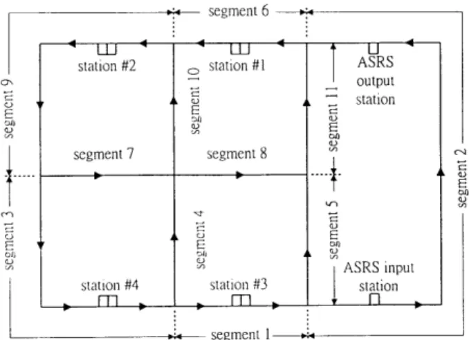
Based on the modelling procedure presented in [17], a complete robust AGVS flow-path model can be constructed by putting basic nets together. A flow-path layout given by Sriniv-asan et al. [6] is used to illustrate the proposed modelling procedure. The layout is presented in Fig.1(a). The robust PN flow-path model of the given layout is constructed and presented in Fig.1(b). The model constructed by the proposed method can be easily verified to be robust by structural property analysis using the technique given in Murata [22]. The verifi-cation results indicate that the model is structurally bounded (i.e. 1-bounded, and safe), strictly conservative, repetitive, con-sistent and structurally live.

2.2 CTPN System Model

Hsieh [18] proposed a modelling procedure for constructing a CTPN system model. The modelling procedure includes three steps:

1. To incorporate coloured tokens and timed transitions into the PN flow-path robust model.

2. To generate vehicle movement sequence by introducing command places and command tokens to the model. 3. To compute the reachable marking at time t⫹1 by adding

the product of a coloured incident matrix and a firing sequence to the marking at time t.

A complete CTPN system model can thus be obtained. Coloured tokens in the CTPN system model represent the entities of vehicles, workpieces and their statuses. Timed tran-sitions are used to measure the performance time of the

(3)

vehicles. Timed places are used to measure the process time of the machine. Command places are used to receive management commands that, in turn, direct the vehicles to move. Figure 1(c) shows the CTPN system model of the given illustrated layout.

3. Flexible System Management Module

To enhance AGVSimNet off-line simulation and on-line moni-toring and control capabilities, besides the CTPN system model, a flexible system management module is necessary. The man-agement module performs three major tasks including: 1. Vehicle dispatching.

2. Vehicle routeing. 3. Traffic control.

Unlike the common simulation model, several special functions are added to the module.

3.1 Vehicle Dispatching

According to Egbelu and Tanchoco [19], the vehicle dis-patching rules fall into two categories. The first disdis-patching rule category is a decision that involves the selection of a vehicle from a set of idle vehicles and the assignment of a unit load pickup task to the selected vehicle. The secondary dispatching rule category is a decision that involves the selec-tion of a work centre from a set of centres and a simultaneous request for the service of a vehicle. In AgvSimNet, the unit load throughput is used as a measure of rule performance. The user may choose an assignment rule from both the work-centre initiated task assignment rules and the vehicle initiated task assignment rules. If one vehicle is available and several jobs are waiting, the vehicle initiated task rule will be triggered. On the other hand, if one job is waiting and several vehicles are available, the work centre initiated task rule will be trig-gered. When several jobs are waiting and several vehicles are available, if work centre priority is higher than vehicle priority, it is treated as single-work multi-vehicle problem. If vehicle priority is higher than work centre priority, it is treated as single-vehicle multi-work problem.

The work centre initiated task assignment rules include the random vehicle (RV) rule, the nearest vehicle (NV) rule, the farthest vehicle rule, the longest idle vehicle rule, and the least utilised vehicle (LUV) rule. The vehicle initiated task assign-ment rules include the random work centre (RW) rule, the shortest travel time (or distance) (STT/D) rule, the longest travel time (or distance) (LTT/D) rule, the maximum outgoing queue size (MOQS) rule, the minimum remaining outgoing queue space (MROQS) rule, the first come first served (FCFS) rule, the unit load shop arrival time (ULSAT) rule, the modified first come first served (MFCFS) rule [19], the MOD FCFS [6] rule, and the MIX [21] rule.

3.2 Vehicle Routeing

When a vehicle is selected for a specified task, AgvSimNet has to determine one possible route for the vehicle based upon

a certain criterion. Usually, AgvSimNet estimates the travel time/distance of all possible routes and determines the best one. A from/to table is generated and stored in the simulation model. 3.3 Traffic control

In a guide-wired system, the vehicle travel velocity is pre-planned based on the given flow-path layout. Since the zone control function is employed, collisions are avoided in normal operation. A travelling vehicle will stop whenever another vehicle is detected in the zone ahead. To make the assigned vehicles move to the destinations, vehicles blocking their way have to be pushed away. In AgvSimNet, three different methods are used to clear the vehicle blocking. These methods are: 1. To push ahead the blocking vehicle one zone.

2. To move the blocking vehicle to one of the specified zones near a station.

3. To move the blocking vehicle to the nearest rest area if there is one.

In AgvSimNet, when a blocking situation occurs, method one is used first. If the blocking situation remains, then method two is used. If method two is not effective, method three is used to remove the blocking.

Since the zone control function is used in AgvSimNet, it may cause the assigned vehicle to move in a stop–go manner when it is needed to push a vehicle away. Since the stop–go mechanism may damage the mechanical parts of vehicles, it is advisable to avoid it. Because of that, a two-step-ahead-forecast mechanism is adopted in many guide-wired systems. In AgvSimNet, the two-step-ahead-forecast function is adopted and implemented in the system. An assigned vehicle will not move unless the forward two-step zones are clear. In AgvSim-Net, when two vehicles arrive at the same traffic control point (e.g. an intersection or a merge) at the same time, the right at the crossroad is usually given to the vehicle on the right-hand side.

4. Dynamic Vehicle Dispatching Scheme

It is known that a vehicle-dispatching rule usually works well for a specific level of throughput, but may not work so well when the level of throughput is changed. The user can connect AgvSimNet to an AGVS controller and select an on-line dynamic dispatching control mode. When a given time period is passed, AgvSimNet will automatically evaluate the vehicle dispatching rule by quickly executing on-line system simula-tions for various possible vehicle dispatching rules. A suitable vehicle-dispatching rule will be selected to replace the original one to perform the task in the next time period. The schematic diagram of an on-line dynamic vehicle dispatching control strategy is shown in Fig. 2.

5. AgvSimNet Structure

AgvSimNet includes four major modules, namely, the input module, the model generator module, the system management

(4)

Fig. 1. (a) The floor-path of a given layout [6], (b) The PN floor-path model of the given layout. (c) The CTPN system model of the given layout.

Fig. 2. Schematic diagram of an on-line dynamic vehicle dispatching strategy.

Fig. 3. AgvSimNet system structure.

Fig. 4. A plant layout.

module and the output module. The on-line dynamic vehicle-dispatching scheme is included in the system management module. The structure of AgvSimNet is presented in Fig. 3. The system management module has been described above, and the other modules are detailed below.

5.1 Input Module

This module is a query-and-answer module. The module is designed so that users can key in the AGVS information for modelling. Four types of information are generally required:

(5)

Fig. 5. Initial flow-path layout design.

1. Flow-path layout.

2. Physical entities and attributes. 3. Mode switch.

4. Job schedule and management rules.

5.1.1 Flow-path Layout

The user is asked to input the flow-path layout by keying in the combination of L, D, M, and I, and some other numbers. L, D, M and I represent line, divide, merge, and intersection nets, respectively. Numbers represent path directions. For example, “I1423” represents an intersection net with input paths one from the left and one from the button, and output paths one to the right and one to the top.

5.1.2 Physical Entities and their Attributes

The user is asked to provide the total number of vehicles in the system, the velocity of each vehicle, the type of load, total number of stations, the location of each station, associated pick-up/delivery buffers and buffer sizes, loading/unloading time, process time, and the length of each path-segment.

5.1.3 Mode Switch

AgvSimNet has three different modes – simulation, on-line monitoring and real-time dynamic dispatching control. On the simulation mode, the user performs simulations to conduct system performance evaluation. In the on-line monitoring AgvSimNet is connected to AGVS controllers (i.e. programm-able logic controllers). AgvSimNet updates and displays current AGVS status once every two seconds. In the real-time dynamic dispatching control mode, searching will carry on for the suitable vehicle dispatching rule for the system. Therefore, it is possible to maintain the optimal performance of the AGVS.

5.1.4 Job Schedule and Management Control Rules

The user is asked to input job types, production process and job arrival frequency, and to choose one type of vehicle dispatching and routeing rule and a traffic control method.

5.2 Model Generation Module

In this module, a CTPN system model is systematically con-structed. This module contains two parts, the CTPN system model and the database for storing the information of system elements.

CTPN model: This part constructs the CTPN model, the col-oured incident matrix of the model, and a from–to chart that describes all possible routes from a station to all other stations. System database: The system database is used to store the data or information of all system elements and their attributes (i.e. the number of available vehicles, current status of each vehicle, etc.).

5.3 Coloured Tokens and Timed Transitions/Places When the vehicles in AgvSimNet are given different job assignments or located at different positions, the vehicle func-tions become different. Therefore, it is necessary to give vehicle identification. In AgvSimNet, the combinations of nine different colours and four different shapes (circle, square, rhombus and oval) are used as the colours of vehicle tokens to represent 36 different vehicles. Besides vehicle identification, vehicle states are modelled. Three different colours, green, cyanine and magenta, are used to represent different vehicle states, namely, free, assigned but empty, and loaded, respectively. The colour of the vehicle-state is inserted in the centre of a vehicle token as a smaller size of the same shape. An ordinary place, represented by a circle, is used to represent a path segment. A timed place, represented by a rectangle, is used to represent a station. In the neighbourhood of a station place, a rectangle appears with three numbers inside it. The first number shows the completed time of the current job. The second and third numbers shows the numbers of parts in the input buffer and the output buffer, respectively. A narrow empty rectangle is used to represent a timed transition, and a bar, 兩, is used to represent an ordinary transition.

5.3.1 Movement Command Sequence

Once a vehicle is assigned and the route is determined, the movement command sequence is generated. Command places, mk, where k is an integer, are used to receive the movement command tokens. The coloured command token in command places can only be used to guide a vehicle with the same col-our.

5.3.2 Markings Evolution

The coloured incident matrix of the system model is automati-cally established in AgvSimNet. If an event happens, it may cause the firing of transitions. That will result in a token redistribution. The marking of the AGVS is thus evolved based upon the state evolution equation

Mk⫽ Mk⫺1⫹ N S T

where N is an incident matrix, S is a transition firing sequence in the given time interval, and Mk⫺1 and Mk are the markings before and after the firings of S.

(6)

Table 1. Simulation results by AgvSimNet for the first layout given in Srinivasan et al. [6].

Throughput Vehicle FCFS MFCFS STTF MOD FCFS

number

␣f ␣e ␣l Mean ␣f ␣e ␣l Mean ␣f ␣e ␣l Mean ␣f ␣e ␣l Mean

waiting waiting waiting waiting

time time time time

L1.DAT1 1 0.218 0.148 0.634 3.971 0.218 0.146 0.637 3.940 0.218 0.143 0.639 3.712 0.218 0.145 0.637 3.772 L1.DAT2 1 0.329 0.223 0.448 6.230 0.330 0.222 0.448 6.139 0.326 0.205 0.469 5.122 0.329 0.213 0.458 5.342 L1.DAT3 1 0.436 0.299 0.265 12.435 0.438 0.295 0.267 11.893 0.440 0.256 0.304 7.335 0.443 0.270 0.287 8.277 L1.DAT4 1 0.579 0.410 0.011 460.05 0.597 0.392 0.011 375.50 0.653 0.266 0.081 18.025 0.645 0.282 0.072 21.582 L1.DAT5 1 0.580 0.415 0.005 1430.9 Unstable 0.809 0.180 0.011 76.297 0.814 0.174 0.012 74.800

Note: System is assumed to be unstable if the maximum number of jobs in any output buffer reaches 500. ␣f, ␣eand␣l, denote the fraction of time

that a device is travelling loaded, travelling empty and waiting in an idle state, respectively.

5.4 Output Generation Module

In the simulation process, AgvSimNet displays important mation at the top of the animation monitor screen. This infor-mation includes current time, the number of jobs scheduled, the number of jobs done, the number of items of work-in-process, the number of vehicle-trips done, and the number of vehicles being pushed away.

The report generator prints out basic information. The time-domain status tracking on each entity or event is generated upon request. Whenever a user has some specific requirements that are not included in the report, he/she may write his/her report generation program to interface with AgvSimNet.

6. Verification Examples

Two simulation examples, given by Sirinivasan et al. [6], are presented to verify the correctness of the simulation results of AgvSimNet. In Srinivasan et al. [6], three AGVS flow-path layouts are presented to validate the analytic method. In this paper, we intend to use two of these three layouts as examples to validate the correctness of AgvSimNet. Since layout number two is a bi-directional system that is not available yet in AgvSimNet, the layout will not be used here.

Simulation runs are carried out in the environment of AgvSimNet and the results are given in Tables 1 and 3. By comparing the results from AgvSimNet with those from [6] Table 2. Simulation results by Srinivasan et al. [6] for the first layout case.

Throughput Vehicle FCFS MFCFS STTF MOD FCFS

number

␣f ␣e ␣l Mean ␣f ␣e ␣l Mean ␣f ␣e ␣l Mean ␣f ␣e ␣l Mean

waiting waiting waiting waiting

time time time time

L1.DAT1 1 0.189 0.139 0.672 3.433 0.189 0.139 0.672 3.425 0.189 0.135 0.675 3.261 0.189 0.137 0.674 3.318 L1.DAT2 1 0.323 0.223 0.454 5.833 0.323 0.222 0.455 5.758 0.323 0.208 0.469 4.942 0.323 0.213 0.464 5.222 L1.DAT3 1 0.433 0.301 0.266 11.123 0.433 0.296 0.271 10.349 0.433 0.258 0.309 6.971 0.433 0.270 0.297 7.788

L1.DAT4 1 Unstable Unstable 0.650 0.271 0.078 16.867 0.650 0.290 0.060 21.044

L1.DAT5 1 Unstable Unstable 0.814 0.180 0.005 76.790 0.814 0.182 0.004 61.220

Note: See Table 1 for definitions.

(e.g. Tables 2 and 4), it is obvious that the results from [6] give a lower ratio value on vehicle use. This is due to a more detailed and realistic consideration for a collision-free requirement involving the zone control function and the two-step-ahead forecast function and blocking phenomenon in AgvSimNet. These functions are not considered in [6]. These functions and phenomena require a longer time for a collision-free check and thus elongate the waiting time for vehicle movement a little. In addition to these factors, different algor-ithms for traffic controls may also result in different con-clusions. The differences between the simulation results obtained from AgvSimNet and those of [6] increase as the throughput level increases (DAT1⬍ DAT2 ⬍ DAT3 ⬍ DAT4 ⬍ DAT5). This is due to the number of blocking occurrences and the ratio of blocking time increases as the throughput level increases. Therefore, it is reasonable to conclude that the results obtained from AgvSimNet are more realistic and thus more reliable.

7. Application Examples

To illustrate the effectiveness of AgvSimNet, two off-line design problems (i.e. the flow-path layout design and the dispatching problem), and an on-line dynamic vehicle-dispatching problem are used for comparative study.

(7)

Table 3. Simulation results by AgvSimNet for the third layout given in Srinivasan et al. [6]. Thr ough pu t V eh ic le FCFS MFCFS STTF MOD FCFS num b er ␣f ␣e ␣l ␣b Mean ␣f ␣e ␣l ␣b Mean ␣f ␣e ␣l ␣b Mean ␣f ␣e ␣l ␣b Mean waiting waiting waiting waiting time time time time L3.DAT1 8 0.236 0.211 0.553 0.019 1.577 0.231 0.212 0.551 0.019 1.576 0.236 0.210 0.554 0.019 1.561 0.236 0.211 0.553 0.019 1.572 L3.DAT2 8 0.336 0.300 0.365 0.032 1.789 0.339 0.302 0.360 0.032 1.788 0.339 0.287 0.375 0.031 1.622 0.338 0.292 0.370 0.031 1.721 L3.DAT3 8 0.474 0.423 0.103 0.050 4.872 0.475 0.423 0.102 0.050 5.907 0.479 0.338 0.183 0.047 1.861 0.478 0.373 0.149 0.049 2.489 Note : See Table 1 for definitions. ␣b denotes the fraction of time that a device is blocked when it is travelling. Table 4. Simulation results by Srinivasan et al. [6] for the third layout case. Thr ough pu t N u m be r FCFS MFCFS STTF MOD FCFS of veh icl es ␣f ␣e ␣l ␣b Overall ␣f ␣e ␣l ␣b Overall ␣f ␣e ␣l ␣b Overall ␣f ␣e ␣l ␣b Overall mean mean mean mean waiting waiting waiting waiting time time time time L3.DAT1 8 0.220 0.193 0.587 N/A 1.410 0.220 0.193 0.587 N/A 1.410 0.220 0.192 0.588 N/A 1.405 0.220 0.193 0.587 N/A 1.336 L3.DAT2 8 0.315 0.276 0.409 1.481 0.315 0.277 0.408 1.484 0.315 0.271 0.414 1.442 0.315 0.274 0.410 1.365 L3.DAT3 8 0.443 0.389 0.168 2.176 0.443 0.390 0.167 2.177 0.443 0.347 0.210 1.567 0.443 0.368 0.189 1.670 Note: See Tables 1 and 3 for definitions. N/A means “not available”. In their simulation, vehicle blocking is not considered.

(8)

Table 5. Machining sequence, interarrival and processing time of each product type.

Product Inter- Machining sequence Processing time type arrival

time

A 1000 AS/RS, 1, 3, 2, 4, AS/RS 0, 300, 180, 300, 180, 0 B 900 AS/RS, 3, 2, 4, AS/RS 0, 240, 210, 180, 0 C 800 AS/RS, 1, 3, 4, AS/RS 0, 270 , 240, 240, 0

Table 6. Simulation results for three layout cases.

Layout Simulation time Mean waiting time

number (s) for parts (s)

1 280 841 8621

2 245 025 4905

3 210 279 398

Fig. 6. Design of the second flow-path layout.

7.1 Flow-Path Layout Design Problem

The layout of an AGVS flow-path has a direct effect on the system operation performance. The higher the degree of traffic congestion induced by imbalance in the material flows, the lower is the system performance. Therefore, the design of flow-path layout is important.

Table 7. Simulation results by using STTD.

Vehicle 14 15 16 17 18 19 20 21 22 23 24 number ␣f 31.34 31.23 30.55 30.26 30.01 28.84 27.62 27.08 27.35 26.01 25.05 ␣c 67.92 67.95 66.87 68.67 68.67 67.43 66.11 64.19 61.10 59.50 56.93 ␣l 0.73 0.82 2.58 1.32 1.32 3.73 6.27 8.73 11.55 14.49 18.02 ␣b 2.05 2.38 2.73 4.91 4.91 5.45 5.87 5.53 5.49 5.56 6.18 e – 9.3 4.3 4.8 4.4 1.5 0.1 2.5 4.7 ⫺0.5 ⫺1.1

␣f,␣eand␣l represent the fraction of time that a vehicle is travelling loaded, travelling empty and waiting in an idle state, respectively.␣brepresents the fraction of time that a vehicle is blocked during travelling loaded and travelling empty. e is an improvement index, e is performance improvement index, e ⫽ (simulation time of k⫺1 vehicles ⫺ simulation time of k vehicles)/simulation time of k⫺1 vehicles.

Fig. 7. Design of the third flow-path layout.

Fig. 8. The number of vehicles that pass the path segment during 3000 vehicle trips.

Figure 4 shows a given plant layout. The plant fabricates three different product types, A, B and C. Each product type has its own machining sequence. The machining sequence, interarrival time and processing time of each product type are given in Table 5.

The interarrival time and the processing time of the parts are normally distributed. Their standard deviations are about

(9)

Fig. 9. Simulation results for different vehicle dispatching rules.

Table 8. Task ID numbers and their descriptions. Task ID number Product type Task description

TK1 A to move part from P1 to D2

TK5 B to move part from P1 to D3

TK9 C to move part from P1 to D2

Table 9. The execution time for different vehicle dispatching rules. Dispatching rule Dynamic FCFS MFCFS STTD MOQS MIX

Execution time 6890 9346 9121 6989 9162 7749

15% of the mean values of processing times. The AGVS has the following distinct features:

1. There are four vehicles in the system.

2. Three different vehicle velocities are given (i.e. low⫽0.1, median⫽0.25 and high⫽0.5 in length units/second). 3. The system is of unit load type.

4. The loading/unloading operation usually takes 20 s. The management strategy includes the use of FCFS and LIV vehicle dispatching rules and the shortest distance routeing rule. Simulations are executed by five runs for each design. Each run performs 3000 vehicle trips.

By using the proposed modelling procedure for the given plant layout, a flow-path layout is constructed in Fig. 5. The simulation results reveal that during the 3000 vehicle trips the vehicle flows of path segments 1, 2, 3, 6, and 9 are high (see

Table 6). However, the vehicle flows of path segments 4, 5, 7, 8, 10, and 11 are relatively low. The mean waiting time of the part is large (see Table 7). This is due to the fact that the blocking frequency is too high. By observing the initial flow-path layout, one may find that the vehicle flows of flow-path segments 3 and 9 may decrease if the path directions of segments 4 and 10 are reversed. Therefore, layout 2 can be obtained and is presented in Fig. 6. Based upon the results of the simulation runs for layout 2 (the vehicle flows of segments 7 and 8 are low), layout 3 can be obtained and is presented in Fig. 7. The simulation results of three different layouts are given in Fig. 8 and Table 6. The results show that the flow-path layout markedly affects the performance of the AGVS. It is obvious that layout 3, as compared to the other two layouts, is the design that needs minimum simulation time and least waiting time for parts and least construction cost.

7.2 Vehicle Dispatching Problem

An application example presented by Liu and Duh [21] is used here to illustrate the effectiveness of various vehicle dispatch rules by computer simulations. In Liu and Duh, three different vehicle-dispatching rules, MOQS, STT/D and MIX were presented and the results are compared. In our study, more dispatching rules for the same application are presented. From the results of simulations, we try to select the optimal number of vehicles and the best vehicle-dispatching rule for the given system.

Figure 9 shows the simulation results of AgvSimNet. The results indicate that STTD is the best dispatching rule among all presented rules. Therefore, STTD is used as the dispatching rule for this application. From these simulation runs, the opti-mal number of vehicles required for the system is also determ-ined. Table 7 gives the fractions of vehicle use and the simulation time saved when more vehicles are used in the system. According to the performance improvement index e, this indicates that a reasonable number of vehicles for the given system is between 14 and 18. If the reduction of production time is far more important than the cost of vehicles, the use of 18 vehicles is suggested for the system. If the vehicle cost is of great concern, 14 vehicles are obviously a better choice for the system. The AGVS user may make the selection based on individual needs.

It is obvious that the simulation times presented in Fig. 9 are higher than those in Liu and Duh [21]. This is because Liu and Duh had made the assumption that the spurs of the system are capable of accommodating all vehicles waiting to enter. In AgvSimNet, this assumption is relaxed and made more realistic. Therefore, the blocking problem is allowed to occur and the vehicles travel in a stop–go manner. This results in a longer simulation time.

7.3 On-line Dynamic Vehicle Dispatching Problem Since AgvSimNet is developed based on Petri nets, it is allowed to provide on-line graphical animation for the AGVS. When AgvSimNet is connected to an AGVS controller, it can monitort on-line and report the current status of the system.

(10)

Fig. 10. The on-line dynamic vehicle dispatching control execution process. Thus, on-line dynamic vehicle dispatching control is also

poss-ible if simulations can be executed in real-time.

An on-line dynamic vehicle dispatching control example is presented here. For comparative purposes, the application example of Liu and Duh is used in this study once again. In the previous study, we reached the same conclusion as Liu and Duh, that a reasonable number of vehicles for the given situation is between 14 and 18. Here, 18 vehicles are used for the application to illustrate the effectiveness of the on-line dynamic vehicle dispatching control.

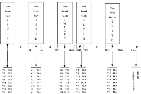
The selection of optimal vehicle dispatching rules is carried out in every time period T. Here, time period T such that it is allowed to perform eight tasks. An identification number is given to each task. Table 8 lists all task identification numbers and their descriptions. The dispatching rule for the first time period is determined on-line by simulating the execution of the first ten tasks with different dispatching rules and then selecting the rule with minimum simulation time. The selected rule is applied to the first eight tasks only. The optimal dispatching rule for the second time period is performed immediately after the first eight tasks are completed. Similarly to time period 1, the time period 2 rule can be determined by simulating the task execution sequence numbers 9 to 18, based upon the current and the forecast information. The selected rule is then applied to the task execution sequence numbers 9 to 16 only. By doing so, the kth time period dispatching rule can be determined, and then eight more tasks are executed.

In order to further explain the on-line dynamic vehicle dispatching control strategy, we trace the processes and record the results for time periods 1, 9, 112, 113 and 170. These records are given in Fig. 10. The total execution time is 6890 time units and the total number of time periods is 375. Three thousand tasks (i.e. vehicle trips) are completed. For comparison purposes, Table 9 gives the execution times of this study and simulations with the FCFS, MFCFS, STTD, MOQS and MIX rules obtained in the previous study. The tabulated results indicate that the on-line dynamic dispatching control strategy is the best one among the given set of vehicle

dis-patching rules since it gives the minimum execution time to complete 3000 trips.

8. Conclusions

In addition to strong simulation capability, AgvSimNet provides three distinct features including animated performance visual-isation, on-line vehicle monitoring and on-line dynamic vehicle dispatching control. The user does not need any prior knowl-edge of programming since AgvSimNet is a complete simul-ation program generator instead of a simulator toolkit. AgvSim-Net adopts modular PN modelling techniques to construct the simulation model. This guarantees the robustness of the built model. Two verification and three application examples presented in this paper show that AgvSimNet gives satisfactory results for off-line evaluation as well as opening a promising new direction for applying simulators for on-line monitoring and dynamic vehicle dispatching control. Although AgvSimNet is now only good for guide-wired systems, by modifying the modelling technique for free-ranging vehicle systems, in future, it can be extended for free-ranging AGVSs for more general applications.

References

1. B. Duffau and C. Bardin, “Evaluating AGVS circuits by simul-ation”, Proceedings of 3rd International Conference on Automated Guided Vehicle Systems, pp. 229–245, 1985.

2. M. Anderson, “AGV system simulation – a planning tool for AGV route layout”, Proceedings of the 3rd International Conference on Automated Guided Vehicle Systems, pp. 291–295, 1985. 3. P. J. Egbelu and J. M. A. Tanchoco, “Potentials for bidirectional

guidepath for automatic guided vehicle systems”, International Journal of Production Research, 24, pp. 1075–1099, 1986. 4. C. M. Harmonosky and R. P. Sadowski, “A simulation model and

analysis: integrating AGVs with non-automated material handling”, Proceedings of the 1984 Winter Simulation Conference, pp. 341– 348, 1984.

(11)

5. W. L. Maxwell and J. A. Muckstadt, “Design of automatic guided vehicle systems”, IIE Transactions, 14, pp. 114–124, 1982. 6. M. M. Srinivasan, Y. A. Bozer and M. Cho, “Trip-based material

handling systems: through put capacity analysis”, IIE Transactions, 26(1), pp. 70–88, 1994.

7. R. J. Gaskins and J. M. A. Tanchoco, “AGVSim2 – a development tool for AGVS controller design”, International Journal of Pro-duction Research, 27, pp. 915–926, 1989.

8. R. J. Gaskins, J. M. A. Tanchoco and F. Taghboni, “Virtual flow paths for free-ranging automated guided vehicle systems”, International Journal of Production Research, 27, pp. 91–100, 1989. 9. P. J. Egbelu, “The use of non-simulation approaches in estimating vehicle requirements in an automatic guided vehicle based trans-port system”, Material Flow, 4, pp. 17–32, 1987.

10. D. A. Davis, “Modeling AGV systems”, Proceedings of the 1986 Winter Simulation Conference, Alexandria, VA, pp. 568–574, 1986. 11. R. J. Gaskins and J. M. A. Tanchoco, “Flow path design

for automated guided vehicle systems”, International Journal of Production Research, 25, pp. 667–676, 1987.

12. P. Matzener, “System simulation – a very important engineering and decision making tool”, Proceedings of 6th International Con-ference on Automated Guided Vehicle Systems, pp. 77–87, 1988. 13. E. B. Quinn, “Simulation based system for automatic development and testing of AGV control software”, Proceedings of the third International Conference on Automated Guided Vehicle Systems, pp. 219–227, 1985.

14. R. E. King and K. S. Kim, “AgvTalk: An object-oriented simulator for AGV systems”, Computers and Industrial Engineering, 28(3),

pp. 575–592, 1995.

15. T. Araki, T. Takahashi, M. Suekane and M. Kawai, “Flexible AGV system simulator”, Proceedings of the 5th International Conference on Automated Guided Vehicle Systems, pp. 77–86, 1987.

16. S. Hsieh and Y. J. Shih, “Automated guided vehicle systems and their Petri-net properties”, Journal of Intelligent Manufacturing, 3, pp. 379–390, 1992.

17. S. Hsieh and Y. J. Shih, “The development of an AGVS model by the union of the modulised floor-path nets”, International Journal of Advanced Manufacturing Technology, 9, pp. 20–34, 1994.

18. S. Hsieh, “Synthesis of AGVS by coloured-timed Petri nets”, International Journal of Computer Integrated Manufacturing, 11, pp. 334–346, 1998.

19. P. J. Egbelu and J. M. A. Tanchoco, “Characterization of automatic guided vehicle dispatching rules”, International Journal of Pro-duction Research, 22, pp. 359–374, 1984.

20. I. Sabuncuoglu and D. L. Hommertzheim, “Dynamic dispatching algorithm for scheduling machines and automated guided vehicles in a flexible manufacturing system”, International Journal of Pro-duction Research, 30(5), pp. 1059–1079, 1992.

21. C.-M. Liu and S.-H. Duh, “Study of AGVS design and dispatching rules by analytical and simulation methods”, International Journal of Computer Integrated Manufacturing, 5(4&5), pp. 290–299, 1992.

22. T. Murata, “Petri nets: properties, analysis and applications”, Proceedings of the IEEE, 77(4), pp. 541–580.