The Backend Design of an Environmental Monitoring System upon Real-Time Prediction of Groundwater Level Fluctuation under the Hillslope

TITLE:

The Backend Design of an Environmental Monitoring System upon Real-Time

Prediction of Groundwater Level Fluctuation under the Hillslope

Authors and Affiliates:

Hsueh-Chun Lin, Corresponding Author, Writing

Assistant Professor, Department of Health Risk Management, China Medical University, 91 Hsueh-Shi Rd., Taichung, 40402, Taiwan, R.O.C., Telephone: 886.4.22053366 ext 6506, Fax: 886.4.22070429, E-Mail: snowlin@mail.cmu.edu.tw

Yao-Ming Hong, Corresponding Author, Concept

Assistant Professor, Department of Environment and Disaster Management, Ming Dao University, 369 Wen-Hwa Rd., Peetow, Changhua 52345, Taiwan, R.O.C. Telephone: 886.4.8876660ext 8614, Fax: 886.4.8879012. E-Mail: blueway@mdu.edu.tw

Yiao-Chiang Kan, Concept, Consultant

Assistant Professor, Department of Communications Engineering, Yuan Ze University, No. 135 Yuan-Tung Road, Chung-Li, Tao-Yuan, Taiwan 32003, R.O.C

ABSTRACT

The groundwater level represents a critical factor to evaluate hillside landslides. A monitoring system upon the real-time prediction platform with online analytical functions is important to forecast the groundwater level due to instantaneously monitored data when the heavy precipitation raises the groundwater level under the hillslope and causes instability. This study is to design the backend of an environmental monitoring system with efficient algorithms for machine learning and knowledge bank for the groundwater level fluctuation prediction. A Web-based platform upon the MVC-based (model-view-controller) architecture is established with technology of Web services and engineering data warehouse to support online analytical process and feedback risk assessment parameters for real-time prediction. The proposed system incorporates models of hydrological computation, machine learning, Web services, and online prediction to satisfy varieties of risk assessment requirements and approaches of hazard prevention. The rainfall data monitored from the potential landslide area at Lu-Shan, Nantou and Li-Shan, Taichung, in Taiwan, are applied to examine the system design.

Keywords: real-time prediction platform, groundwater level, MVC-based architecture, engineering data

1. Introduction

Prediction of the groundwater level under hillslope after a precipitation is an important risk assessment factor for landslide hazard prevention. An automatic and efficient assessment procedure for landslide detection includes monitoring, transporting, collecting, analyzing rainfall data as well as forecasting groundwater level in order to save time, property and life of residents before the landslide occurs (Ahmadi and Sedghamiz, 2007). Therefore, it is quite helpful to design a rainfall data analysis mechanism at the backend of an environmental monitoring system which can instantly predict the groundwater level under the hillslope for decision support.

The groundwater level is a significant factor to predict the possibility of landslide (Mantovani et al., 2000). Thus the rainfall intensity is an important element to affect the level of groundwater. Caris and van Asch (1991) conducted the geotechnical and hydrological surveys on a small landslide in black marl material to reveal the critical threshold of landslide when the groundwater level is 4m below the ground surface. It was measured that deeper landslides (5–20m depth) are the most cases triggered by pore pressures on the slip plane due to a rising groundwater level (van Asch et al., 1999). The slope with potential landslide requires a realistic estimation of groundwater levels according to a variety of parameters such as infiltration, shear strength, groundwater and steepness. These parameters could be driven into the modeling algorithms for accurate slope-stability analyses of pre-existing landslides (Neaupane and Achet, 2004; Trigo et al., 2005). Hence, a precise and real-time prediction of groundwater level may help forecasting occurrence of the landslide. The prediction model can be simulated by learning correlations of monitoring data and historical records. It is straightforward to recognize the relationship between groundwater level and precipitation by field measurement. McDonald and Harbaugh (2003) developed the governing equations to simulate the groundwater flow and estimate its level by using MODFLOW, which is the well-known groundwater flow model based on the finite difference equation (Rushton and Redshaw, 1979). Within the MODFLOW, if the parameters such as hydraulic conductivity and specific storage were accurately measured, then the groundwater level could be forecasted (Hunt et al., 2008). Unfortunately, some parameters of the necessary analysis are usually absent to cause difficulties for iterative procedures in the application software. Accordingly, many studies designed the Web-based information system with interoperability between disparate sources and visualized interface to interpret the interaction among the various water cycle components by using feedback loops in a dynamics environment, and then created a model to simulate responses of different irrigation management scenarios (Googal et al., 2008; Khan et al., 2009).

In the mountain area, landslides usually occur just a few hours after the torrential precipitation. It is expected to predict groundwater levels hourly and suggest appropriate value of influence variables by learning historical on-site monitored data. To manipulate the data, the backend of monitoring system responds in driving the hydraulic data into the knowledge bank for efficient computation and risk assessment. Hence, the Web-based platform with extendible real-time functions is quite eligible to provide online risk information management for decision support and hazard alert. Many approaches of integrated system were developed with computation tools to simulate the hydrological models and analyses for environmental monitoring (Foran et al., 2000; Causapé, 2009; Horsburgh et al., 2009; Xing et al., 2009; Worm et al., 2010). Furthermore, a flexible and expandable framework with Web interface would be more competitive to incorporate heterogeneous data. Thus, most of the commercial packages provide full application but they still require customization. Stewart and Mohamed (2004)

had investigated several built-in frameworks for validating the interrelationship between the perspectives and indicators, and suggested that the system upon a fundamental of expandable framework can be practiced to customize the functionalities. To access instantaneous rainfall data and historical precipitation records by considering integrity and transparency of the system, the MVC (model-view-controller) design pattern is eligible to contribute a solid architecture for incorporating various computation models with centralized administration. In addition, the Web platform enables users carry out manipulations in distributed sites. Therefore, a number of emerging technologies including distributed objects, intelligent agents, internet and Web-based technologies have been proposed to implement collaborative product design systems (Shen et al., 2003). Technology of Java and extensible markup language (XML) can support cross-platform design and distributed-data integration for Web services. Furthermore, metadata with XML schema can be serialized within the document and be parsed by the application programming interface (API) of Java to match requirements of data transformation and online computation (Hagemann, 1999). Instead of stand-alone software, many Web-based products were developed to integrate distributed, heterogeneous resources into an open system (Xiao et al., 2001).

In this study, we proposed a forecasting model of groundwater level fluctuation at the backend of the real-time monitoring system. Rainfall data due to torrential precipitation are involved in the database of the system to yield a knowledge bank beyond the simulation. The hybrid nonlinear algorithm based on Darcy’s law is employed to calculate the groundwater flux rate. The historical rainfall data are contributed for the machine learning by the efficient iteration procedures to calibrate prediction parameters of groundwater level. Finally, the MVC-based architecture is implemented for the Web-based platform to process the monitored data. The data acquired from the hillslopes of Lu-Shan and Li-Shan in Taiwan were practiced for risk assessment.

2. Technology and Methodology

This study emphasizes the backend design of the environmental monitoring system which contains the frontend devices with wireless sensor network (WSN) and the backend platform for real-time online analysis. In order to access the monitored rainfall data and forecast the groundwater level beyond precipitation on the hillslope, the methodology involves the hydrological analysis model to enable the machine learning process to support the functionalities of real-time decision and online prediction. Herein, the proposed system consists of four units: 1) the hydrological continuity algorithm, 2) the risk assessment index by machine learning, 3) the Web platform upon MVC-based architecture, and 4) the online decision support for real-time prediction. The Java technology with open source APIs is employed to construct the necessary Web-based system.

2.1 Hydrological Continuity Algorithm

When the precipitation occurs, it falls into the ground and infiltrates into the soil; then, water reaches the aquifer region and flows into the downstream along the impervious layer. The hydrological process with infiltration steps can be illustrated in Figure 1 and the well-known hydrological continuity equation (Chow et al., 1988) can be recruited to simulate the process as follows:

O I dt dS _{= −}

In which, S is the groundwater storage of control volume, I is the inflow rate that includes the infiltration recharge rate and the groundwater inflow rate, O is the groundwater outflow rate. Equation (1) denotes the groundwater storage in an aquifer region of unit area required for a unit rise of the water table (Sophocleous, 1991; Maréchal et al., 2006; Park and Parker, 2008; Hong, 2008). It is also affected by the porosity:

dt dh pL dt

dS = (2)

where p is the fillable porosity for volume of water per unit area L. The equation implies a numerical process that the groundwater can flow into the identical linear unit reservoirs stepwise. The inflow rate can be written as:

g p I

I

I = + (3)

where Ip and Ig represents the infiltration recharge rate and the groundwater inflow rate, respectively. Based on Eq. (4), the infiltration recharge rate is formed by multiplying the unit area L with parameters: the precipitation rate Pr, the evapotranspiration rate Er, the overland flow Or, and the soil keeping water rate Sr.

(

)

[

]

I_p = _r− _r + _r + _r (4)

Herein, the infiltration rate and extra inflow may gradually decrease when the precipitation stops.

Furthermore, the extra groundwater inflow is from the infiltration recharge of upstream watershed and can be estimated with the linear reservoirs method below (Hong and Wan, 2010):

(

)

[

]

∑

Giving the corresponding parameters: K is a transportable parameter of groundwater, A is a constant depending on the groundwater watershed area, α represents the infiltration ratio of precipitation, Pm is the depth of precipitation during the time interval between (m-1)Δt and mΔt, H is the function of time t in Eq. (6) to represent a unit pulse of infiltration recharge rate with the storage constant β and the number n of unit reservoirs.

( )

₍

₎

It implies that the parameter β and n may result in long time duration and a low peak pulse of infiltration recharge rate. Thus, the peak pulse of infiltration recharge rate Hp and the peak time tp can be obtained as tp = β(n-1) by differentiating H(t). The symbol N is denotes as the influence range of infiltration pulse recharge rate depending on the parameters β and n for simplifying the equation denotations.

Substituting Equations (2), (4) and (5) into (1), then dividing the equation by pL, it yields

(

)

[

]

∑

Where, the positive parameter I (=α(A+1)/p) is defined as the “Rise Number” while the negative parameter K is defined as the “Sink Number”. Thus, the first term Kh at the right side of the equation represents the head loss of groundwater level and the second term is the infiltration recharge and extra groundwater inflow. Herein, Eq. (7) yields the first-order linear differential equation and is a function of variables t and h. This equation involves the constant recharge rate Wt between time t and t+Δt, i.e.,

∑

[

(

)

]

= Δ + − = N m m t _{P H N m t} W 1

t t t t IW Kh t h h _{= +} Δ − Δ + (8)

Where, h=ht is the initial condition of groundwater level and the approximate ht+Δt due to ht can be derived from Eq.(8). Hence, the theoretical solution can be applied for this study.

2.2 Risk Assessment Indexes for Machine Learning

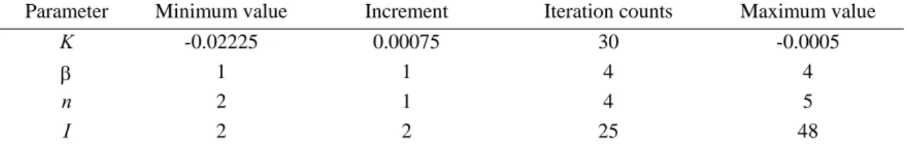
As monitoring, the rainfall data were collected by the frontend devices and transported to the backend server as the base of the engineering data warehouse. The data warehouse is known as an integral database for historical data repository behind systematic arrangement by information technique (Inmon, 1996). Bill Inmon defined it as an integrated, subject-oriented, time-variant and non-volatile database that provides support for decision making (Inmon and Kelley, 1994). The fact table and correspondent cube dimensions are the essential components to generate the schema of data warehouse. The fact table contains facts that link with their dimensions, thus the cube dimensions provide metadata of the facts through their attributes. Moreover, the raw data in various formats can be rigorously unified by the extract-transform-load (ETL) procedure into database through extraction, consolidation, filtering, transformation, cleansing, conversion and aggregation (Rob and Cornel, 2005). The critical factor leading to the use of data warehouse can perform complex queries and analyses without slowing down the operating system. The engineering data warehouse in this study accumulates the hydrological data with respect to computation of groundwater level and precipitation for machine learning. Based on Equation (5), we can obtain the necessary forecast parameters K, β, n and I through training the historical precipitation data and practicing the newly monitored data. Meanwhile, these parameters are eligible for the attributes of relations within database to yield the fact tables. The historical precipitation data are requested for the training process to feedback the optimal parameters as the risk assessment indexes for the predictive groundwater level and become the knowledge bank.

As follows, we review the literatures and estimate the factors to determine the important groundwater parameters for machine learning.

(1) Period of infiltration recharge rate (n, β) – the parameters control the travel time period of infiltration recharge rate according to Eq. (6). In the other word, the time lag of groundwater travel period can be a function of the thickness of unsaturated zone, rainy seasons and precipitation intensity. Some monitored data showed that the time lag for the peak precipitation and the peak groundwater level may bring into half day to twenty days (van Asch et al., 1999; Lee et al., 2006; Park & Parker, 2008).

(2) Rise number (I) – the number stands for the rising level of groundwater level under precipitation and is an artificial variable determined by fillable porosity (p) and infiltration ratio of precipitation (α), which are given in Eq.(2) and (5), respectively. Both of p and α can be studied from rainfall events (Sophocleous, 1991; Li et al., 2005; Bhark & Small, 2003). The ratio α/p was suggested by nonlinear regression to minimize the root mean square (RMS) deviation between observed and predicted water levels for the calibration period (Park & Parker, 2008).

(3) Sink number (K) – the number is another artificial variable, similarly, to determine the sinking level of groundwater level. In this study, we refer the groundwater parameters in Table 1 determined by the previous

study and create the risk assessment indexes to execute the machine learning loops.

Table 1 Groundwater parameters used in machine learning (Hong and Wan, 2010)

Parameter Minimum value Increment Iteration counts Maximum value

K -0.02225 0.00075 30 -0.0005

β 1 1 4 4

n 2 1 4 5

I 2 2 25 48

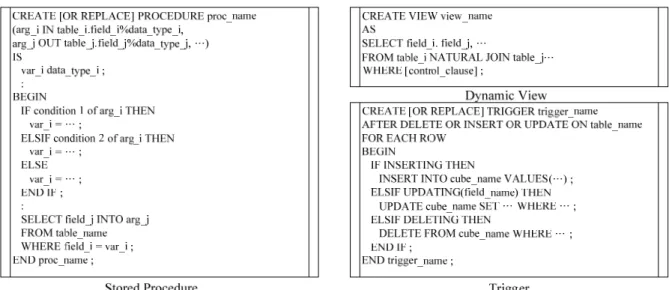
Herein, we implement the risk assessment indexes above with training data for the machine learning mechanism. As incorporating the diverse engineering data, we propose the control modules by considering three primary database components, dynamic view, stored procedure and trigger, to generate dimensional cubes through PL/SQL (Procedural Language/Structured Query Language) scripts. These scripts are executed by the functions developed in the database server for data access. Then the transaction progress in the web server can automatically retrieve analytical results by triggering these functions for advanced computation.

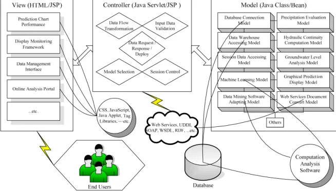
2.3 Web Platform upon MVC-based Architecture

To construct the Web platform for real-time prediction, a concept of MVC-based architecture would be implemented at the backend of system to progress the online analysis by acquiring rainfall data of precipitation from the monitoring facilities at the frontend. The architecture reflects the model-view-controller (MVC) design pattern that includes several design patterns, which was initially discovered from Smalltalk-80 in 1970’, to describe proven strategies for building reliable object-oriented software system (Krasner and Pope, 1988). The public of design patterns was first made available by Gamma et al. (1994) to introduce twenty-three patterns related to creational, structural and behavioral models for software design to progress recurrent elements. The MVC theoretically hybrids three of them, the strategy, observer, and composite patterns, and divides system responsibilities into three parts: the model, which maintains program data and logic; the view, which provides a visual presentation of the model; the controller, which processes user input and makes modifications to the model. The framework with MVC paradigm controls the consuming computation resources when the user is not interacting with the interface and avoids unnecessary performance loss (Shan, 1989).

Figure 2 illustrates the conceptual infrastructure in three main blocks containing the components of model, view and controller, which provide individual modules with mutual supports based on system requirements. The models of precipitation evaluation, hydraulic continuity computation, and groundwater level analysis work with monitored rainfall data and previous algorithms to conduct the machine learning model. Furthermore, they feed back the forecast parameters for showing prediction diagrams with the model of graphical prediction display. According to this architecture, we apply the open source framework to build the system prototype for online data process of precipitation. This framework can customize more reusable supports than enterprise commercial modules because plenty of free APIs reduce complexity in Web application software development. The system employs prediction components with flexible functionality and user-friendly interface.

2.4 Online Decision Support for Real-time Prediction

of network boom-up era (Chaudhuri and Dayal, 1997). It provides efficient functionalities with computation algorithm on the backbone of data warehouse to explore historical data. In this study, we propose the OLAP function as the online computation model to bridge the web and database servers for analyzing the precipitation data and risk assessment indexes beyond the real-time prediction. The risk indexes of the groundwater parameters for OLAP can be accessed with the database server while the monitored rainfall data are queried from the data warehouse. The procedure remains complex queries behind machine learning but presents simple data transactions through dynamic views in the data warehouse. The design implies the load balancing algorithm that spreads the load across multi-node Web servers and receives all requests from the frontends to achieve the scalability (Colajanni and Yu, 1997; Brendel et al., 1998). Bartra and Li (2007) recently configured of clustered Web services nodes for accessing a common database by implementing a data virtualization layer at each node to abstract instances and balance loads of the database from Web service applications. Herein, the proposed OLAP upon the MVC-based architecture design follows the similar concept: the Web server and database server would be independent but communicated with Web services and help optimizing the load balance between both servers to improve system integration and performance.

Due to this approach, the system requests information diagrams for online decision support and prediction through light-weight data process to avoid laggardly accessing heavy data. The light-weight data such as risk criteria are transformed as Web services documents with XML standards while the heavy historical precipitation data are analyzed by the hydrological algorithm for machine learning. Hence, simple data transaction is remained in the Web server while necessary dynamic views or dimensional cubes are created in the data warehouse of the database server for complex data query. Hence the requirements for real-time efficiency and loading balance at the backend of system can be ensured on the Web and database servers.

3. System Analysis and Design

In order to approve the system design with the given methodology for the practical problems, we simulated rainfall data monitored by either the traditional equipments or WSN facilities settled in the landslide areas at Li-Shan, Taichung and Lu-Shan, Nantou, in Taiwan, for training historical precipitation data.

3.1 Requirement Analysis

Two stages are considered for training precipitation data: (A.) Execute machine learning with the daemon computation in server based on hydrological algorithms to feedback optimal parameters into database; (B.) process client data through OLAP by accessing the knowledge bank for decision support. The stage a presides over calculation in variety of historical records by simulation and analysis tools, and the stage B presents instant prediction results from dynamic view.

In this study, the platform is designed at the backend of the monitoring system to receive surveillance data prior to database and conduct machine learning with the hydrologic analysis modules beyond the groundwater level prediction. Following approaches are considered: (1) Acquire monitored data from the surveillance stations with automatic control; (2) Administrate the data flow with integrity and transparency; (3) Practice online analysis with real-time computation; (4) Collaborate historical precipitation records with machine learning for

decision support; and (5) Customize management functions upon the expandable framework for further study. The proposed system requires to aggregate diverse precipitation data and a model of decision support is grouped by object-oriented modules. Based on MVC design, this functional model can be expanded due to advanced requirements and the controller can manage data interaction between client and server sites. In addition, the Web services provide mechanism of data transformation to integrate heterogeneous database.

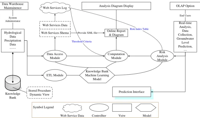
3.2 Infrastructure Design

The collaboration diagram of the MVC-based architecture herein is controlled with four modules: “data access,” “computation,” “ETL,” and “risk analysis” to organize the knowledge bank model. The infrastructure is illustrated in Figure 3 that is implementing the objects shown in Figure 2. In the figure, the system design paradigm consists of MVC components with symbols of model, view and controller which are presented by the blocks of hexagon, rectangle and eclipse, respectively. Mutual supports for individual objects are activated by solid lines while analytical modules and Web services documents are correlated by dashed lines for accessing light-weight data. Behind this architecture, each component supplies unique functionality but works together to build a flexible and expandable web-based platform. The model library will be generated with the data warehouse of historical precipitation data for online computation. For example regarding Fig. 2 and Fig. 3, the “data access module” controls the models of “database connection,” “session data accessing,” and “Web services document conversion”; the “ETL module” manage “data warehouse accessing” and “data mining software adapting” models; the “computation module” conducts the models of “machine learning,” “groundwater level analysis,” and “hydraulic continuity computation”; the “risk analysis module” executes “precipitation evaluation” and “graphic prediction display” models as well as communicates with Web services log. All models will achieve integration of machine learning, data conversion, decision support, and online diagram below.

3.2.1 Machine Learning

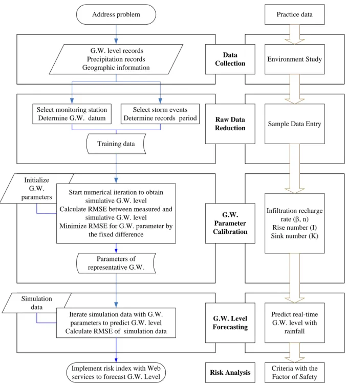
The machine learning model provides hydrologic computation for training historical precipitation data. Based on the derived hydrological continuity formulation, we can simply to develop a computation module for solving the differential equations. Figure 4 depicts the algorithm with four major stages of data collection, raw data reduction, groundwater parameter calibration, and groundwater level forecasting to obtain feedback of the prediction parameters and complete risk analysis of the groundwater level.

(1) Data collection – the precipitation and the groundwater level are recorded with the sampling interval of one or two hours. Geographic information including topography, location and depth of well, and location of rainfall station can be rendered to determine the groundwater datum. The suitable wells will offer obvious response when precipitation occurs. For this manner, we chose one well from the traditional monitoring station installed in Li-Shan area and one well from the WSN facilities installed in Lu-Shan area.

(2) Raw data reduction – the raw data contain historical records. The storm with maximum cumulative precipitation volume will be the candidate sample for training. The proper groundwater level records of wells compared with each well are selected to present the relationship between groundwater level and precipitation. Finally, a series of training samples are obtained according to the chosen storm records. Herein, we selected the

precipitation data of the strong typhoon Haitang and Tailim during July and August in 2005 for study.

(3) Groundwater parameter calibration – the calibration of a flow model refers to models with capability of producing field-measured heads and flows. In the proposed system, the groundwater level at the (i+1)th time step, say hi+1, is carried out by the computation module due to the derived differential equations, and the iteration is converged by the root mean square error (RMSE), Ep, as following equation:

(

)

∑

where n is the number of records in a storm; hpi+1 and hmi+1 are the predicted groundwater level and the measured groundwater level at the (i+1) time step, respectively. The optimal approach will occur when the groundwater parameters yields the minimum RMSE. In this study, the selected precipitation data of typhoons were trained and the groundwater parameters were calibrated for simulation.

(4) Groundwater level forecasting – the representative values of groundwater parameters are plugged into the iteration. The real-time groundwater level at the next time step can be estimated according to the precipitation depth and the groundwater level at the current time step till the RMSE reaches the convergent criteria. We used rainfall data of other typhoons, Matsa and Longwang, during August and September in 2005 to simulate real-time data and predict the groundwater level by using the parameters due to machine learning.

Once the machine learning flow is completed, we can estimate the stability of hillslope by parameters of soil property such as friction angle, soil density, condensation force and consider the popular formula of factor of safety (FS) given below for the landslide criterion of risk analysis (Skempton and DeLory, 1957).

(

)

where, hw is groundwater level (m), C is effective condensation force (N/m2), g is gravity (=9.81m/s2), φ is

friction angle, θ is slope angle, D is thickness of soil layer (m), ρs and ρw are the saturation soil density and the

water density (kg/m3), respectively.

3.2.2 Web Services

Due to the infrastructure, the functions of data conversion, decision support and online diagram are required to support Web services for presenting the prediction interface.

A. Data Conversion

The model loads instantaneously monitored data or historical precipitation data with ETL process into the data warehouse as well as supports uniform standard of data logs for machine learning or feedback of threshold tables. It follows several ways for data transaction: 1.) create connections to different database for routine data query; 2.) convert data files with compatible format for assistant software; 3.) transform reporting data as typical XML document through web services. For example, as considering surveillance data of Lu-Shan and Li-Shan areas, the historical precipitation records were imported into the data warehouse. The trained data were converted as unified format in the data logs and uploaded to the server. As activating the machine learning, the computation process was executed in daemon mode. A set of coefficients was created and saved in the criteria

log when the learning was completed. Then, the risk index table of groundwater level was updated by criteria and real-time rainfall data could be simulated by corresponding coefficients for online prediction process. Herein, these simulation results will be discussed in the next section.

B. Decision Support

We design the decision support model with efficient database algorithm to manipulate environmental assessment indexes and feedback for the knowledge bank. The database functions such as dynamic views or stored procedures, which allow triggering automatic data processing for data mining, can immediately respond assessment factors for decision making. Figure 5 shows the pseudo codes of model that queries hydrological data and categories them into various dimensions within the data warehouse. Meanwhile, the model supports the prediction formula to request the groundwater parameters from knowledge bank after the system is trained by historical precipitation records. Herein, the expected groundwater level can be estimated by several hours before the real-time rainfall data cause the level to reach the threshold. In this study, the criteria of groundwater level for Lu-Shan and Li-Shan were learned after precipitation data of typhoons were imported into database. Similarly, the newly monitored data can be loaded into the knowledge bank for next forecasting.

C. Online Diagram

The design of online diagram function for Web services implements free Java APIs, “jfreechart,” into the library of models for better performance for browsing decision support information on the Web-based system. The graphical chart of rainfall and groundwater level is created by either querying data source through database or parsing criteria from XML documents. With adaptive array data arrangement embedded within this model, the output chart controlled by Java Servlet is transformed as image data stream based on JPEG format through I/O interface. According to the system management, for instance, the result data and curves associated with decision diagram can be referred to the specified hillslope if the groundwater level reaches the critical index.

In general, the machine learning model trains the historical precipitation data to attain the groundwater parameters. These coefficients can be adopted through Web services to simulate new rainfall data. The automatic transformation procedure is designed to process the schema of Web services efficiently while incorporating machine leaning results and real-time monitored data.

4. Results and Discussions

In the past years, typhoons often brought heavy precipitation to cause landslides in areas of Lu-Shan and Li-Shan, and lots of wells were mounted for different types of facilities to monitor the groundwater level. The topographies of Lu-Shan and Li-Shan are shown in Figure 6(a) and (b), respectively, in which the monitored data from the wells B03 (Lu-Shan) and B-9 (Li-Shan) are selected for this study. A suitable elevation was chosen as the virtual datum according to the records of groundwater level. The average depth is about 7.75m (B03) and 19.52m (B-9) above virtual datum, thus, the similar groundwater depth condition is expected for all of the wells. In this practice, we loaded historical precipitation records of typhoons at hillslope of these areas into data warehouse for machine learning. Then, the real-time monitored rainfall datasets caused by new coming typhoons were used to examine the system design. In both areas, precipitation more than 100mm per day could happen about 7~8 times from May to September. Precipitation information of chosen landslide areas is described below.

(1) Lu-Shan: The precipitation with depth 486.5mm caused by typhoon Haitang during 18-31th July 2005 was selected for machine learning; then the rainfall data monitored from typhoon Matsa during 4-9th August in the same year were simulated for prediction. (2) Li-Shan: The precipitation with depth 287.5mm caused by typhoon Tailim from 26th August to 6th September in 2005 was adopted for training system; one month later, the rainfall data collected from typhoon Longwang between 26th September and 7th October were simulated for prediction.

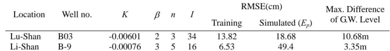
Table 2 Groundwater parameters and RMSE of wells RMSE(cm)

Location Well no. K β n I

Training Simulated (Ep)

Max. Difference of G.W. Level

Lu-Shan B03 -0.00601 2 3 34 13.82 18.68 10.68m

Li-Shan B-9 -0.00076 3 5 16 6.53 49.4 3.35m

The proposed system trains the historical precipitation data and restores the representative coefficients of groundwater with RMSE in the log files at Web server. Then, they can readily support for online simulation via Web services when new rainfalls happen. Table 2 displays the rise number I, the sink number K and other parameters for both wells in which the maximum difference of groundwater level (MDGL) is 10.68m (B03) and 3.35m (B-9). In general, the large rise number implies that the storm quickly raise the groundwater level under hillslopes while the small sink number induces the slow recession rate of groundwater level. Therefore, the large MDGL at Lu-Shan results from a fast rise speed with the large I as well as a fast sink speed with large -K, and vice versa for simulation at Li-Shan. With these parameters, the online diagram model allows the predictive curve of groundwater level at various time steps. The screen shots shown on Figure 7(a) and (b) display the plots of real-time rainfall distribution (bar) corresponding to comparison of the prediction (dash line) and monitored groundwater level (solid line) with similar approach. The diagrams of both hillslope areas explain that the groundwater level climbed up after the storm became strong; and then it reached the peak when the rainfall tended to be easy. Besides of real-time rainfall information, the decision support model forecasts the tendency of groundwater level a few hours before the monitored data reaches the threshold.

We can simply substitute the predictive groundwater level into the formula given in Eq. (10) to estimate the factor of safety of landslide as the threshold. When the precipitation occurs, the arising rate of groundwater level is quite important for predicting how long to reach the threshold. In this study, the machine learning model trains historical precipitation to create proper rise number I and sink number K, and then the mechanism of Web services allows real-time data simulation for online prediction. Furthermore, these parameters can result in diverse criteria by training more types of rainfall data such as considering characteristics of local precipitation, duration of rain season, soil water potential of hillslope, or initial groundwater level. Therefore, the design of monitoring system is capable of real-time prediction for online hazard alert.

5. Conclusion Remark

This study accomplishes the backend design of an environmental monitoring system with MVC-based architecture which incorporates on-site monitored data and historical precipitation records for engineering data warehouse as well as implements online analytical processes for predicting the groundwater level under hillslope. The primary components of the platform backend involve reusable models of machine learning and Web services to approve capability of real-time prediction for risk assessment and decision support. With practical field tests,

the objectives are reached as follows: 1) predict the groundwater level by simulating rainfall data with machine learning; 2) employ Web services for processing real-time risk assessment information; 3) generate the infrastructure of engineering data warehouse upon MVC-based architecture for dispersed data resource; 4) administrate the monitoring system with remote control mechanism for virtual centralized management. In the future, the developed real-time functions for predicting groundwater level fluctuation can help enhance analysis of stability of hillslope.

Acknowledgement

The author would like to thank the research support from China Medical University (project number CMU95-199 and CMU96-153) and the National Science Council of the Republic of China (project number 98-2625-M-451-001).

References

1. Ahmadi, S.H., & Sedghamiz, A. (2007). Geostatistical Analysis of Spatial and Temporal Variations of Groundwater Level. Environmental Monitoring and Assessment, 129, 277-294

2. van Asch, Th.W.J., Buma, J., & Van Beek, L.P.H. (1999). A view on some hydrological triggering systems in landslides. Geomorphology, 30, 25-32.

3. Batra, V.S., & Li, W.S. (2007). Web services database cluster architecture. U.S. Patent Publication, US 0203944 A1.

4. Bhark, E.W., Small E.E. (2003). Association between plant canopies and the spatial patterns of infiltration in shrubland and grassland of the Chihuahuan Desert, New Mexico. Ecosystems 6, 185–196.

5. Brendel, J., Kring, C.J., Liu, Z., & Marino, C.C. (1998). World-wide-web server with delayed resource-binding for resource-based load balancing on a distributed resource multi-node network. United States Patent 5774660.

6. Caris, J.P.T., & van Asch, T.W.J. (1991). Geophysical, geotechnical and hydrological investigations of a small landslide in the French Alps. Engineering Geology, 31 (3-4), 249-276.

7. Chaudhuri, S., Dayal, U. (1997). An Overview of Data Warehousing and OLAP Technology. ACM SIGMOD Record, 26(1), 65-74.

8. Chow, V. T., Maidment, D.R., & Mays, L.W. (1988). Applied hydrology, McGraw-Hill, Singapore, 242-264.

9. Colajanni, M., & Yu, P.S. (1997). Adaptive TTL schemes for load balancing of distributed Web servers. ACM SIGMETRICS Performance Evaluation Review, 25(2), 36-42.

10. Foran, J., Brosnan, T., Connor, M., Delfino, J., DePinto, J., Dickson, K., Humphrey, H., Novotny, V., Smith, R., Sobsey, M., & Stehman, S. (2000). A Framework for Comprehensive, Integrated, Watershed Monitoring in New York City. Environmental Monitoring and Assessment, 24, 147-167.

11. Gamma, E., Helm, R., Johnson, R., & Vlissides, J. (1994). Design Patterns: Elements of Reusable Object-Oriented Software. Addison-Wesley.

to web services for the National Water Information System. Environmental Modelling and Software, 23, 404-411.

13. Hagemann, D. (1999). XML and JAVA: Engineering Software Development Meets Internet Technologies. Proceedings of the ASME Design Technical Conferences, Las Vegas, Nevada, 12-15.

14. Hong, Y. M. (2008). Graphical estimation of detention pond volume for rainfall of short duration. Journal of Hydro-environment Research, 2, 109-117.

15. Hong, Y. M. & Wan, S. (2010), Forecasting groundwater level fluctuations for rainfall-induced landslide, Natural Hazards, DOI: 10.1007/s11069-010-9603-9

16. Hunt, R.J., Prudic, D.E., Walker, J.F., & Anderson, M.P. (2008). Importance of unsaturated zone flow for simulating recharge in a humid climate. Ground Water, 46(4), 551-560.

17. Inmon, B., & Kelley, C. (1994). The Twelve Rules of Data Warehouse for a Client/Server World. Data Management Review, 4(5), 6-16.

18. Inmon, W.H. (1996). Building the Data Warehouse, 3rd Ed. Wiley & Sons.

19. Khan, S., Luo, Y., & Ahmad, A. (2009). Analysing complex behaviour of hydrological systems through a system dynamics approach. Environmental Modelling and Software, 24, 1363-1372.

20. Causapé, J. (2009). A computer-based program for the assessment of water-induced contamination in irrigated lands. Environmental Monitoring and Assessment, 158, 307-314.

21. Krasner, G.E., & Pope, S.T. (1988). A cookbook for using the model-view-controller user interface paradigm in Smalltalk-80. Journal of Object-Oriented Programming, 1(3), 26-49.

22. Lee, L.J.E., Lawrence, D.S.L., & Price, M. (2006). Analysis of water-level response to rainfall and implications for recharge pathways in the Chalk aquifer, SE England, Journal of Hydrology, 330, 604-620. 23. Li, W.D. (2005). A Web-based Service for Distributed Process Planning Optimization. Journal of

Computers in Industry, 56 (3), 272-288.

24. Mantovani, F., Pasuto, A., Silvano, S., & Zannoni, A. (2000). Collecting data to define future hazard scenarios of the Tessina landslide. Int’l J. Applied Earth Observation and Geoinformation, 2(1), 33-40. 25. Maréchal, J.C., Dewandel, B., Ahmed, S., Galeazzi, L., & Zaidi, F.K. (2006). Combined estimation of

specific yield and natural recharge in a semi-arid groundwater basin with irrigated agriculture. Journal of Hydrology, 329, 281-293.

26. McDonald, M.G., & Harbaugh, A.W. (2003). The history of MODFLOW. Ground Water, 41, 280-283. 27. Neaupane, K.M., & Achet, S.H. (2004). Use of backpropagation neural network for landslide monitoring: a

case study in the higher Himalaya. Engineering Geology, 74, 213-226.

28. Park, E., & Parker, J.C. (2008). A simple model for water table fluctuations in response to precipitation. Journal of Hydrology, 356, 344-349.

29. Xing, L.T., Wu, Q., Ye, C.H., & Ye, N. (2009). Groundwater environmental capacity and its evaluation index. Environmental Monitoring and Assessment, DOI 10.1007/s10661-009-1163-7.

30. Rob, P., & Cornel, C. (2005). Database Systems: Design, Implementation and Management, Ch12. Tomson Course Technology, 6th ed.

Sussex, UK.

32. Shan, Y.P. (1989). An event-driven model-view-controller framework for Smalltalk. Conference Proceedings on Object-oriented Programming Systems, Languages and Applications. New Orleans, Louisiana, United States, 347–352.

33. Shen, W., & Wang, L. (2003). Web-based and agent-based approaches for collaborative product design: an overview. International Journal of Computer Applications in Technology, 16 (2-3), 103-112.

34. Skemptom, A. W., and Delory, F.A., (1957), Stability of natural slopes in London Clay, ASCE journal, 2, 378-381

35. Sophocleous, M. (1991). Combining the soil water balance and water level fluctuation method to estimate natural groundwater recharge: practical aspects. Journal of Hydrology, 124, 229-241.

36. Stewart, R.A., & Mohamed, S. (2004). Evaluating web-based project information management in construction: capturing the long-term value creation process. J. Automation in Construction, 13 (4), 469-479.

37. Trigo, R.M., Zêzere, J.L., Rodrigues, M.L., & Trigo, I.F. (2005). The influence of the North Atlantic Oscillation on rainfall triggering of landslides near Lisbon. Natural Hazards 36, 331–354.

38. Worm, G.I.M., van der Helm, A.W.C., Lapikas, T., van Schagen, K.M., & Rietveld, L.C. (2010). Integration of models, data management, interfaces and training support in a drinking water treatment plant simulator. Environmental Modelling and Software, 25, 677-683.

39. Xiao, A., Choi, H.J., Kulkani, R., Allen, K.J., Rosen, D., & Mistree, F. (2001). A Web-based Distributed Product Realization Environment. Proceedings of ASME 2001 Design Engineering Technical Conferences, Pittsburgh, PA, USA, DETC00/ CIE-14624.

Figures ove_rlan d flo_w precipitation evapotranspiration infiltration impervious layer groundwate_{r level} evaporation

Figure 1 Groundwater travel process from precipitation to stream

OLAP Option Analysis Diagram Display

Data Warehouse Maintainence Prediction Interface Real-time Analysis, Data Collection, Groundwater Level Prediction, … Online Report & Diagram System Administrator Knowledge Bank

Web Services Shema Provide XML file

Web Services Data Web Services Log

Threshold Criteria Hydrological Data Precipitation Data …… Data Access Module Risk Analysis Module Computation Module Knowledge Bank Machine Learning Model

Risk Index Table

End Users

ETL Module

Stored Procedure Dynamic View

Symbol Legend

Web Service Data Controllter Veiw Model

Address problem

Select monitoring station Determine G.W. datum

G.W. level records Precipitation records Geographic information

Select storm events Determine records period

Initialize G.W.

parameters Start numerical iteration to obtain simulative G.W. level

Calculate RMSE between measured and simulative G.W. level

Minimize RMSE for G.W. parameter by the fixed difference

Training data

Parameters of representative G.W.

Simulation data

Iterate simulation data with G.W. parameters to predict G.W. level Calculate RMSE of simulation data

Raw Data Reduction G.W. Parameter Calibration G.W. Level Forecasting Data Collection

Implement risk index with Web

services to forecast G.W. Level Risk Analysis

Environment Study

Sample Data Entry

Infiltration recharge rate ( , n) Rise number (I) Sink number (K)

Predict real-time G.W. level with

rainfall

Criteria with the Factor of Safety

Practice data

Figure 5 – Pseudo code for creating dimensions of hydrological data

Figure 6(a) – Topographic map of landslide at Lu-Shan, Nantou, Taiwan B01 Rainfall B04 B07 B02 _B03 B06 B10 B05 B09 Rain station Groundwater

S W E N 0 1 Kilometers 1600 2200 2150 2100 2050 2050 2000 1950 1900 1850 1800 1750 1700 1650 1550 1500 1450 1400

B9

Figure 7(a) – The online prediction approach of groundwater level at Lu-Shan