門檻隨機波動方法下的風險值估計：以期貨及ETF為例

行政院國家科學委員會專題研究計畫 成果報告

門檻隨機波動方法下的風險值估計：以期貨及 ETF 為例

研究成果報告(精簡版)

計 畫 類 別 ： 個別型

計 畫 編 號 ： NSC 100-2410-H-004-061-

執 行 期 間 ： 100 年 08 月 01 日至 101 年 07 月 31 日

執 行 單 位 ： 國立政治大學財務管理學系

計 畫 主 持 人 ： 杜化宇

計畫參與人員： 碩士班研究生-兼任助理人員：沈容光

大專生-兼任助理人員：曾俐雯

博士班研究生-兼任助理人員：陳苡文

報 告 附 件 ： 出席國際會議研究心得報告及發表論文

公 開 資 訊 ： 本計畫涉及專利或其他智慧財產權，2 年後可公開查詢

中 華 民 國 102 年 01 月 31 日

中 文 摘 要 ： 在本研究中，我們使用可描述厚尾特性的 Stochastic

volatility 模型來探討隔夜訊息對於風險值(VaR)估計值的

影響。透過對於隔夜訊息會影響日間報酬的驗證，我們使用

可描述厚尾特性的 Stochastic volatility(SV)模型來探討

是否隔夜訊息會影響 VaR 的估計對稱的影響效果。假若隔夜

訊息的影響證實不存在，則傳統使用 stochastic

volatility 模型來估計 VaR 是可接受。否則，新的 SV 模型

(或其中一個特例模型)應使用來估計 VaR，才能有效反應市

場訊息的影響。本研究考慮數種可描述厚尾特性的 SV 模型，

並使用較強韌的貝斯 Markov-chain Monte Carlo (MCMC)方

法來估計 THSV 模型中的係數。Deviance Information

Criterion (DIC)使用來作模型的優劣比較。最後，兩種回溯

測試(backtests) (DQ test 與 Berkowitz＇s (2001)

distribution and tail forecast test)使用來探討 VaR 的

績效表現。

中文關鍵詞： 風險值；隨機波動模型；MCMC；回溯測試

英 文 摘 要 ： In this study, we are concerned about the impact of

overnight information (news) on the estimation of

Value-at-Risk (VaR). The past studies showed that the

overnight information can predict the forthcoming

open-to-close daily returns. Based on the result,

this study develops a new VaR model based on the

stochastic volatility with various fat-tailed

distributions. The new SV model can reflect the

effect of overnight information (news) and capture

simultaneously the asymmetries in good and bad news.

Stock index futures and four types of commodity

futures are examined and the MCMC method, which is a

Bayesian and simulation-based estimation method, is

employed for inference and parameter estimation. The

Deviance Information Criterion (DIC) is used as a

criterion for model comparison. Finally, two backtest

methods (DQ test and Berkowitz＇s (2001) test) are

used to evaluate the out-of-sample performance of the

SV-based VaR model.

英文關鍵詞： Keywords: Value-at-Risk； Stochastic Volatility

Model； MCMC； Backtest

Value-at-risk Estimation with Threshold Stochastic

Volatility Model: Futures and ETFs

1. Introduction

Volatility forecasts are important inputs into risk management models (Brooks and Persand

(2003)). It is well known that many financial time series exhibit volatility clustering whereby

volatility is likely to be high when it has recently been high and volatility is likely to be low when it

has recently been low. Generalized autoregressive conditional heteroscedastic (GARCH) models are

conventionally used for modeling time-varying conditional volatility and GARCH models are

extensively used by both researchers and practitioners.

An alternative way to model time varying volatility is to use a discrete-time stochastic volatility

(SV) model (Taylor, 1982, 1986)

①

. One such version was introduced in Taylor (1982) where returns

were defined as a product of two stochastically independent processes. The stochastic volatility model

proposed by Taylor (1982) can be written as

(1)

(2)

(3)

Where

is the time series of interest and

and

are stochastically independent white-noise

processes. Adding an error term

in the dynamics of volatility introduces another source of

randomness in the model that may improve the description of the actual volatility. Taylor‘s (1982)

original formulation assumes that both

and

are equal to zero. The AR(1) process with the time

series innovation

defined in equation (1) accounts for a possible autoregressive relationship in

.

The threshold-type of SV models was first studied by Li and Lam (1995). Possible asymmetric

①

behaviour of stock（and also futures）returns during bear and bull markets is captured by a threshold

model with conditional heteroscedasticity. The results in Li and Lam (1995) showed that the

conditional mean structure could depend significantly on the rise and fall of the market in the previous

day. In addition, many researchers argued that variance responds asymmetrically to the past returns.

An asymmetric effect is produced because variance tends to be higher under the influence of bad news

than under the influence of good news. This phenomenon was pointed out by Black (1976), Christie

(1982), French et al. (1987), Schwert (1989), Campbell and Hentschel (1992) and Cheung and Ng

(1992). Black (1976) and Christie (1982) gave the ‘leverage effect’ as an explanation.

Asymmetric variance has also been considered in the stochastic volatility framework; see, for

example, Danielsson (1994) and Harvey and Shephard (1996). The former used a similar specification

as in Nelson (1991) and the latter allowed for contemporaneous correlation between

and

in (1)

to model the leverage effect. Harvey and Shephard (1996) discovered a significant negative

correlation between

and

in the CRSP data used in Nelson (1991).

This study developes a new THSV-based Value-at-Risk (VaR) model. It can reflect the effects of

news shocks (good news and bad news) and thus capture simultaneously the asymmetries in mean and

variance. The linear structures in (1) and (3) are generalized into threshold non-linear structures (Tong

and, 1980; Tong, 1983, 1990) where the autoregressive dynamics of the mean and variance

components are governed by past realizations. The new SV model is called the threshold stochastic

volatility (THSV) model by So et al. (2002), as shown in the later section.

Value at Risk (VaR) is one of the most important measures of the market risk that has been used for

financial risk management. However, most models in the past literature focus on the computation of

the VaR for negative returns. Indeed, it is assumed that traders or portfolio managers have long trading

positions, i.e. they bought the traded asset and are concerned when the price of the asset falls. In this

study we focus on modeling VaR for futures defined on long and short trading positions. Thus we

model VaR for traders having either position of long futures or short futures. In the first case, the risk

comes from a drop in the futures price of the asset, while the trader loses money when the futures

price increases in the second case.

2. Methodology

（1）symmetric SV model

The stochastic volatility model proposed by Taylor（1982）can be written as

0 1 1 t t t

r

=

ψ

+

ψ r

_-

+

y

(1)

,

~

(0,1)

t t t t

y

=

h u

u

N

(2) 2 1

log

h

_t+

=

α φ

+

log

h

_t

+

η

_t

,

η

_t

~

N

(0,

σ

)

(3)

Where

r

_t is the time series of interest and

u

_t and

η

_tare stochastically independent white noise processes.

Taylor’s (1982) original formulation assumes that both

ψ

₀and

ψ

₁are equal to zero. The AR(1) process with the

time series innovation

y

_t defined in equation (1) accounts for a possible autoregressive relationship in

r

_t.

（2）asymmetric in the mean-only SV model

00 10 1 1 01 11 1 1

0

0

t t t t t t t

ψ

ψ r

y r

r

ψ

ψ r

y r

- --

-ì

+

+

<

ïï

=

_íï

+

+

?

ïî

(1)’

,

~

(0,1)

t t t t

y

=

h u

u

N

(2)’ 2 1

log

h

_t+

=

α φ

+

log

h

_t

+

η

_t

,

η

_t

~

N

(0,

σ

)

(3)’

（3）asymmetric in the variance-only SV model

0 1 1 t t t

r

=

ψ

+

ψ r

-

+

y

(1)’’

,

~

(0,1)

t t t t

y

=

h u

u

N

(2)’’ 0 0 1 2 1 1 1 1

log

0

log

~

(0,

)

log

0

t t t t t t t t

α

φ

h

η r

h

η

N

σ

α

φ

h

η r

-+

-ì

+

+

<

ïï

=

_íï

+

+

?

ïî

(3)’’

（4）the full THSV model

00 10 1 1 01 11 1 1

0

0

t t t t t t t

ψ

ψ r

y r

r

ψ

ψ r

y r

- --

-ì

+

+

<

ïï

=

_íï

+

+

?

ïî

(1)’’’

,

~

(0,1)

t t t t

y

=

h u

u

N

(2)’’’ ₁ 0 0 1 2 1 1 1

l o g

0

l o g

~

( 0 ,

)

l o g

0

t t t t t t t t

α

φ

h

η r

h

η

N

σ

α

φ

h

η r

-+

-ì

+

+

<

ïï

=

_íï

+

+

?

ïî

(3)’’’

3. Value at Risk for Long and Short positions

To emphasize applications in risk management, we estimate the VaR to measure the risk of an investment

position. VaR summarizes the expected maximum loss over a target horizon within a given confidence level

α

. For

the above models, the one-step-ahead VaR forecast at November 29, 2005 to November 29, 2010 for long trading positions is given by long t t α t

VaR

=

μ

+

z

h

(4) 1 short t t α t

VaR

=

μ

+

z

_-

h

(5)

where

z

_α being the left quantile at

α

% for the different distribution and

z

_{1 α}- is the right quantile at

α

%. If the

0

t

μ <

and

|

z

_α

| |

>

z

_1-α

|

, the VaR for long trading position will be larger (for the same conditional variance) than

the VaR for short trading positions. When

μ >

_t

0

is positive, we have the opposite results.

Note：公式（4）和（5）可参考论文 Giot P, and Laurent S, Value-at-risk for long and short trading positions, Journal of Applied Econometrics, 2003, 18: 641-664.

4. Empirical results

0 20 40 60 80 100 120 140 160 1999-11 2000-05 2000-11 2001-05 2001-11 2002-05 2002-11 2003-05 2003-11 2004-05 2004-11 2005-05 2005-11 2006-05 2006-11 2007-05 2007-11 2008-05 2008-11 2009-05 2009-11 2010-05 2010-11 P ri c e ( U S D )

Figure 1 Price series of crude oil futures contract

This empirical investigation examines daily prices (trading days) from November 29, 1999 to November 29, 2010 for the crude oil futures markets. The simulation observations (in sample) and predict observations (out of sample) are from November 29, 1999 to November 29, 2005 and November 30, 2005 to November 29, 2010, respectively. The time series of futures prices is created based on the close price of the nearest contract to maturity

and up to the last trading day for the period before the delivery month. The futures returns are measured by the first

difference of the natural logarithm of the close prices, i.e.

R

_t



ln(

P P

_{t t1}

)

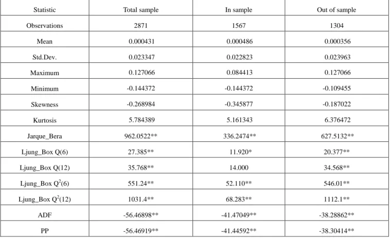
. The summary statistics of returns of

crude oil contracts on in sample, out of sample and the total observations in Table 1 below. Table 1 Summary statistics of returns for crude oil contract.

Statistic Total sample In sample Out of sample

Observations 2871 1567 1304 Mean 0.000431 0.000486 0.000356 Std.Dev. 0.023347 0.022823 0.023963 Maximum 0.127066 0.084413 0.127066 Minimum -0.144372 -0.144372 -0.109455 Skewness -0.268984 -0.345877 -0.187022 Kurtosis 5.784389 5.161343 6.376472 Jarque_Bera 962.0522** 336.2474** 627.5132** Ljung_Box Q(6) 27.385** 11.920* 20.377** Ljung_Box Q(12) 35.768** 14.000 34.568** Ljung_Box Q2(6) 551.24** 52.110** 546.01** Ljung_Box Q2(12) 1031.4** 68.283** 1112.1** ADF -56.46898** -41.47049** -38.28862** PP -56.46919** -41.44592** -38.30414** * Significant at 5% level. ** Significant at 1% level.

Jarque_Bera is a test statistic for testing whether the series is normally distributed.

ADF and PP indicate respectively augmented Dickey and Fuller and Phillips and Perron unit root tests for whether the series is stationary.

Before going into details of the implementation, we parameterize ₀

t s

ψ

, ₁ t s

ψ

, t s

α

and t s

φ

as 0s_t 0 s_t

ψ

=

ψ

+

δ

1s_t 1 s_t

ψ

=

ψ

+

c

t t s s

α

=

α γ

+

t t s s

φ

=

φ d

+

the case

γ

=

d

=

0

assumes that there is no asymmetry in the variance equation and the case

0

δ

=

c

=

γ

=

d

=

corresponds to the symmetric model. In the two different regimes of the mean and variance

equations, the intercept coefficients differ by the constants

δ

and

γ

respectively. The parameters

c

and

d

represent the increase of the autoregressive coefficient in the mean and variance components respectively.

We simulated the in sample data sets, which are from November 29, 1999 to November 29, 2005, by Bayesian MCMC algorithms. We iterated our algorithms 10,000 times and kept the last 8000 iterates (burn in 2000 iterates) as an approximate posterior sample, where the thin are twenty in the WinBUGS.

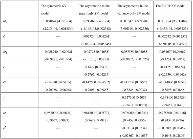
Table 2 Posterior mean, standard deviation (in square brackets) and 90% Bayes interval (in parentheses) from different fitted model for crude oil futures market

The symmetric SV model

The asymmetric in the mean-only SV model

The asymmetric in the variance-only SV model

The full THSV model

0

ψ

0.001044 [4.22E-04] (2.24E-04, 0.001856) 7.02E-04 [9.49E-04] (-1.16E-03, 0.002548) 0.001547 [4.92E-04] (5.90E-04, 0.002536) 0.001284 [9.91E-04] (-6.43E-04, 0.003233)

δ

— 0.002724 [0.001261] (2.88E-04, 0.005245) — 0.002532 [0.001257] (6.09E-05, 0.004971) 1

ψ

-0.058740 [0.02092] (-0.09921, -0.01864) -0.03793 [0.04635] (-0.1301, 0.05213) -0.057580 [0.02085] (-0.09802, -0.01625) -0.034670 [0.04667] (-0.1251, 0.05961)

c

— -0.1479 [0.06436] (-0.2767, -0.02235) — -0.1475 [0.06474] (-0.2739, -0.01962)

α

-0.14070 [0.05135] (-0.26750, -0.06048) -0.142600 [0.04502] (-0.2503, -0.06853) -0.141700 [0.08559] (-0.3325, -0.0032) -0.144000 [0.1054] (-0.3593, 0.02866)

γ

— — -0.327300 [0.2056] (-0.7437, 0.08863) -0.348400 [0.2929] (-0.9455, 0.1640)

φ

0.98200 [0.006604] (0.9657, 0.9923) 0.981800 [0.005774] (0.9679, 0.9912) 0.976000 [0.01241] (0.9458, 0.9956) 0.975800 [0.01416] (0.9454, 0.9976)

d

— — -0.03104 [0.0234] (-0.07867, 0.01657) -0.033890 [0.03457] (-0.1043, 0.02809)

根据表 2，我们所估计的四种模型（Data from November 29, 1999 to November 29, 2005）的表达式可表示为 （1）symmetric SV model

1

0.001044

0.058740

t t t

,

~

(0,1)

t t t t

y

=

h u

u

N

2 1

log

h

_t+

= -

0.140700

+

0.982000log

h

_t

+

η

_t

,

η

_t

~

N

(0,

σ

)

（2）asymmetric in the mean-only SV model

1 1 1 1

0.000702

0.037930

0

0.003426

0.185830

0

t t t t t t t

r

y

r

r

r

y

r

- --

-ì

-

+

<

ïï

=

_íï

-

+

?

ïî

,

~

(0,1)

t t t t

y

=

h u

u

N

2 1

log

h

_t+

= -

0.142600

+

0.981800log

h

_t

+

η

_t

,

η

_t

~

N

(0,

σ

)

（3）asymmetric in the variance-only SV model 1

0.001547

0.057580

t t t

r

=

-

r

_-

+

y

,

~

(0,1)

t t t t

y

=

h u

u

N

1 2 1 1

0.141700

0.976000 log

0

log

~

(0,

)

0.469000

0.944960 log

0

t t t t t t t t

h

η r

h

η

N

σ

h

η r

-+

-ì -

+

+

<

ïï

=

_íï

-

+

+

?

ïî

（4）the full THSV model

1 1 1 1

0.001284

0.034670

0

0.003816

0.182170

0

t t t t t t t

r

y

r

r

r

y

r

- --

-ì

-

+

<

ïï

=

_íï

-

+

?

ïî

,

~

(0,1)

t t t t

y

=

h u

u

N

₁ 1 2 1

0 . 1 4 4 0 0 0

0 . 9 7 5 8 0 0 l o g

0

l o g

~

( 0 ,

)

0 . 4 9 2 4 0 0

0 . 9 4 1 9 1 0 l o g

0

t t t t t t t t

h

η r

h

η

N

σ

h

η r

-+

-ì -

+

+

<

ïï

=

_íï

-

+

+

?

ïî

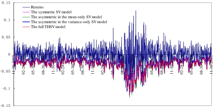
根据 VaR 的计算公式，基于以上四种模型的样本外（Out of sample）每日 VaR（Data from November 30, 2005 to November 29, 2010）与样本收益序列的比较图如下：

-0.15 -0.1 -0.05 0 0.05 0.1 0.15 1 1 -3 0 -2 0 0 5 0 2 -2 8 -2 0 0 6 0 5 -3 0 -2 0 0 6 0 8 -3 0 -2 0 0 6 1 1 -3 0 -2 0 0 6 0 2 -2 8 -2 0 0 7 0 5 -3 0 -2 0 0 7 0 8 -3 0 -2 0 0 7 1 1 -3 0 -2 0 0 7 0 2 -2 9 -2 0 0 8 0 5 -3 0 -2 0 0 8 0 8 -3 0 -2 0 0 8 1 1 -3 0 -2 0 0 8 0 2 -2 8 -2 0 0 9 0 5 -3 0 -2 0 0 9 0 8 -3 0 -2 0 0 9 1 1 -3 0 -2 0 0 9 0 2 -2 8 -2 0 1 0 0 5 -3 0 -2 0 1 0 0 8 -3 0 -2 0 1 0 1 1 -3 0 -2 0 1 0 Returns

The symmetric SV model

The asymmetric in the mean-only SV model The asymmetric in the variance-only SV model The full THSV model

Figure 2 Value at Risk (VaR) for long position trading at 95% confidence level

-0.15 -0.1 -0.05 0 0.05 0.1 0.15 11-30-2005 01-30-2006 03-30-2006 05-30-2006 07-30-2006 09-30-2006 11-30-2006 01-30-2007 03-30-2007 05-30-2007 07-30-2007 09-30-2007 11-30-2007 01-30-2008 03-30-2008 05-30-2008 07-30-2008 09-30-2008 11-30-2008 01-30-2009 03-30-2009 05-30-2009 07-30-2009 09-30-2009 11-30-2009 01-30-2010 03-30-2010 05-30-2010 07-30-2010 09-30-2010 11-30-2010 Returns

The symmetric SV model

The asymmetric in the mean-only SV model The asymmetric in the variance-only SV model The full THSV model

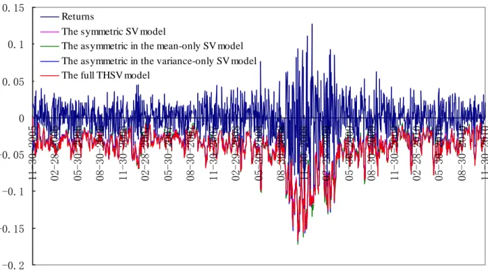
-0.2 -0.15 -0.1 -0.05 0 0.05 0.1 0.15 11-30-2005 02-28-2006 05-30-2006 08-30-2006 11-30-2006 02-28-2007 05-30-2007 08-30-2007 11-30-2007 02-29-2008 05-30-2008 08-30-2008 11-30-2008 02-28-2009 05-30-2009 08-30-2009 11-30-2009 02-28-2010 05-30-2010 08-30-2010 11-30-2010 Returns

The symmetric SV model

The asymmetric in the mean-only SV model The asymmetric in the variance-only SV model The full THSV model

Figure 4 Value at Risk (VaR) for long position trading at 99% confidence level

-0.15 -0.1 -0.05 0 0.05 0.1 0.15 0.2 1 1 -3 0 -2 0 0 5 0 2 -2 8 -2 0 0 6 0 5 -3 0 -2 0 0 6 0 8 -3 0 -2 0 0 6 1 1 -3 0 -2 0 0 6 0 2 -2 8 -2 0 0 7 0 5 -3 0 -2 0 0 7 0 8 -3 0 -2 0 0 7 1 1 -3 0 -2 0 0 7 0 2 -2 9 -2 0 0 8 0 5 -3 0 -2 0 0 8 0 8 -3 0 -2 0 0 8 1 1 -3 0 -2 0 0 8 0 2 -2 8 -2 0 0 9 0 5 -3 0 -2 0 0 9 0 8 -3 0 -2 0 0 9 1 1 -3 0 -2 0 0 9 0 2 -2 8 -2 0 1 0 0 5 -3 0 -2 0 1 0 0 8 -3 0 -2 0 1 0 1 1 -3 0 -2 0 1 0 Returns

The symmetric SV model

The asymmetric in the mean-only SV model The asymmetric in the variance-only SV model The full THSV model

Figure 5 Value at Risk (VaR) for short position trading at 99% confidence level

4. Corresponding parameters’ figures of the four models above

（1）symmetric SV model History:

psi0 2001 4000 6000 8000 10000 -0.001 0.0 0.001 0.002 0.003 psi1 2001 4000 6000 8000 10000 -0.15 -0.1 -0.05 1.38778E-17 0.05 alpha 2001 4000 6000 8000 10000 -0.4 -0.3 -0.2 -0.1 -2.77556E-17 phi 2001 4000 6000 8000 10000 0.94 0.96 0.98 1.0 Density: psi0 sample: 8000 -0.001 0.0 0.001 0.002 0.0 500.0 1.00E+3 psi1 sample: 8000 -0.2 -0.1 0.0 0.0 5.0 10.0 15.0 20.0

alpha sample: 8000 -0.6 -0.4 -0.2 0.0 5.0 10.0 phi sample: 8000 0.94 0.96 0.98 1.0 0.0 20.0 40.0 60.0 80.0 Auto Correlation: psi0 lag 0 20 40 -1.0 -0.5 0.0 0.5 1.0 psi1 lag 0 20 40 -1.0 -0.5 0.0 0.5 1.0 alpha lag 0 20 40 -1.0 -0.5 0.0 0.5 1.0 phi lag 0 20 40 -1.0 -0.5 0.0 0.5 1.0

（2）asymmetric in the mean-only SV model History: psi0 2001 4000 6000 8000 10000 -0.005 0.0 0.005 0.01 psi1 2001 4000 6000 8000 10000 -0.2 -0.1 0.0 0.1 0.2

delta 2001 4000 6000 8000 10000 -0.005 0.0 0.005 0.01 c 2001 4000 6000 8000 10000 -0.4 -0.2 0.0 0.2 alpha 2001 4000 6000 8000 10000 -0.4 -0.3 -0.2 -0.1 -2.77556E-17 phi 2001 4000 6000 8000 10000 0.96 0.98 1.0 Density: psi0 sample: 8000 -0.005 0.0 0.005 0.0 200.0 400.0 psi1 sample: 8000 -0.4 -0.2 0.0 0.0 2.5 5.0 7.5 10.0

delta sample: 8000 -0.005 0.0 0.005 0.0 100.0 200.0 300.0 400.0 c sample: 8000 -0.6 -0.4 -0.2 0.0 2.0 4.0 6.0 alpha sample: 8000 -0.4 -0.3 -0.2 -0.1 0.0 2.5 5.0 7.5 10.0 phi sample: 8000 0.94 0.96 0.98 1.0 0.0 20.0 40.0 60.0 80.0 Auto Correlation: psi0 lag 0 20 40 -1.0 -0.5 0.0 0.5 1.0 psi1 lag 0 20 40 -1.0 -0.5 0.0 0.5 1.0 delta lag 0 20 40 -1.0 -0.5 0.0 0.5 1.0 c lag 0 20 40 -1.0 -0.5 0.0 0.5 1.0 alpha lag 0 20 40 -1.0 -0.5 0.0 0.5 1.0 phi lag 0 20 40 -1.0 -0.5 0.0 0.5 1.0

（3）asymmetric in the variance-only SV model History:

psi0 2001 4000 6000 8000 10000 -0.002 0.0 0.002 0.004 psi1 2001 4000 6000 8000 10000 -0.15 -0.1 -0.05 1.38778E-17 0.05 alpha iteration 2001 4000 6000 8000 10000 -0.6 -0.4 -0.2 5.55112E-17 0.2 phi iteration 2001 4000 6000 8000 10000 0.7 0.75 0.8 0.85 0.9 0.95

gamma iteration 2001 4000 6000 8000 10000 -2.0 -1.0 0.0 1.0 2.0 d iteration 2001 4000 6000 8000 10000 -0.2 -0.1 0.0 0.1 0.2 Density: psi0 sample: 8000 -0.002 0.0 0.002 0.004 0.0 200.0 400.0 600.0 800.0 psi1 sample: 8000 -0.2 -0.1 0.0 0.0 5.0 10.0 15.0 20.0 alpha sample: 8000 -0.6 -0.4 -0.2 0.0 2.0 4.0 6.0 phi sample: 8000 0.9 0.95 1.0 0.0 10.0 20.0 30.0 40.0 gamma sample: 8000 -2.0 -1.0 0.0 0.0 0.5 1.0 1.5 2.0 d sample: 8000 -0.15 -0.1 -0.05 0.05 0.0 5.0 10.0 15.0 20.0 Auto Correlation:

psi0 lag 0 20 40 -1.0 -0.5 0.0 0.5 1.0 psi1 lag 0 20 40 -1.0 -0.5 0.0 0.5 1.0 alpha lag 0 20 40 -1.0 -0.5 0.0 0.5 1.0 phi lag 0 20 40 -1.0 -0.5 0.0 0.5 1.0 gamma lag 0 20 40 -1.0 -0.5 0.0 0.5 1.0 d lag 0 20 40 -1.0 -0.5 0.0 0.5 1.0

（4）the full THSV model History: phi0 2001 4000 6000 8000 10000 -0.005 0.0 0.005 0.01 psi1 2001 4000 6000 8000 10000 -0.2 -0.1 0.0 0.1 0.2

delta 2001 4000 6000 8000 10000 -0.005 0.0 0.005 0.01 c 2001 4000 6000 8000 10000 -0.4 -0.2 0.0 0.2 alpha iteration 2001 4000 6000 8000 10000 -0.6 -0.4 -0.2 5.55112E-17 0.2 phi 2001 4000 6000 8000 10000 0.92 0.94 0.96 0.98 1.0

gamma 2001 4000 6000 8000 10000 -1.5 -1.0 -0.5 0.0 0.5 d 2001 4000 6000 8000 10000 -0.15 -0.1 -0.05 1.38778E-17 0.05 Density: psi0 sample: 8000 -0.005 0.0 0.005 0.0 100.0 200.0 300.0 400.0 psi1 sample: 8000 -0.4 -0.2 0.0 0.0 2.5 5.0 7.5 10.0 delta sample: 8000 -0.005 0.0 0.005 0.0 100.0 200.0 300.0 c sample: 8000 -0.6 -0.4 -0.2 0.0 2.0 4.0 6.0 alpha sample: 8000 -0.75 -0.5 -0.25 0.0 0.0 1.0 2.0 3.0 4.0 phi sample: 8000 0.9 0.95 1.0 0.0 10.0 20.0 30.0

gamma sample: 8000 -2.0 -1.0 0.0 0.0 0.5 1.0 1.5 d sample: 8000 -0.2 -0.1 0.0 0.0 5.0 10.0 15.0 Auto Correlation: psi0 lag 0 20 40 -1.0 -0.5 0.0 0.5 1.0 psi1 lag 0 20 40 -1.0 -0.5 0.0 0.5 1.0 delta lag 0 20 40 -1.0 -0.5 0.0 0.5 1.0 c lag 0 20 40 -1.0 -0.5 0.0 0.5 1.0 alpha lag 0 20 40 -1.0 -0.5 0.0 0.5 1.0 phi lag 0 20 40 -1.0 -0.5 0.0 0.5 1.0 gamma lag 0 20 40 -1.0 -0.5 0.0 0.5 1.0 d lag 0 20 40 -1.0 -0.5 0.0 0.5 1.0

Reference

Asai, M. Bayesian analysis of stochastic volatility models with mixture-of-normal distributions. Mathematics and Computers in Simulation 79, 2579-2596.

Andersen, T., Chung, H. and Sorensen, B. E. (1999). Efficient method of moments estimation of a stochastic volatility model: a Monte Carlo study. Journal of Econometrics, 91, 61-87.

Berkowitz, J. (2001). Testing density forecasts with application to risk management. Journal of Business and Economic Statistics, 19, 465-474.

Black F. (1976). Studies of stock price volatility Changes. Proceedings of the 1976 meetings of the business and economics statistic section, American Statistical Association, 177-181.

Brooks C, Persand G. (2003). Volatility forecasting for risk management. J Forecasting, 22, 1-22.

Campbell JY, Hentschel L. (1992). No news is good news: an asymmetric model of changing volatility in stock returns. Journal of Financial Economics, 31, 281-318.

Cheung YW, Ng L. (1992). Stock price dynamics and firm size: an empirical investigation. Journal of Finance, 47, 1985-1997.

Christie A. (1982). The stochastic behavior of common stock variances: value, leverage and interest rate effects. Journal of Financial Economics, 10, 407-432.

Christoffersen, P. F. (1998). Evaluating interval forecasts. International Economic Review, 39, 841-862.

Danielsson J. (1994). Stochastic volatility in asset price: estimation with simulated maximum likelihood. Journal of Econometrics, 64, 375-400.

Engle, R. F., and Manganelli, S. (2004). CAViaR: Conditional autoregressive value at risk by regression quantiles. Journal of Business and Economic Statistics, 22, 367-381.

French KR, Schwert GW, Stambaugh RF. (1987). Expected stock returns and volatility. Journal of Financial Economics, 19, 3-30.

Gallant, A. R., Hsieh, D. A. and Tauchen, G. E. (1997). Estimation of stochastic volatility models with diagnostics. Journal of Econometrics, 81, 159-92.

Gelfand AE, Smith AFM. 1990. Sampling-based approaches to calculating marginal densities. Journal of The American Statistical Association 85：398-409.

Harvey, A. C., Ruiz, E. and Shephard, N. (1994). Mutivariate stochastic variance models. Review of Economics Studies, 61, 247-64.

Harvey AC., Shephard N. (1996). Estimation of an asymmetric stochastic volatility model for asset returns. Journal of Business and Economic Statistics, 14, 429-434.

Jacquier, E., Polson, N. G. and Rossi, P. E. (1994). Bayesian analysis of stochastic volatility models (with discussion). Journal of Business and Economic Statistics, 12, 371-89.

Kim, S., Shephard, N. and Chib, S. (1998). Stochastic volatility: likelihood inference and comparison with ARCH models, Review of Economics Studies, 65, 361-93.

Liesenfeld, R. and Richard, J. F. (2003). Univariate and multivariate stochastic volatility models: estimation and diagnostics. Journal of Empirical Finance, 10, 505-31.

Li WK, Lam K. (1995). Modelling asymmetry in stock returns by a threshold ARCH model. The Statistician, 44, 333-341.

Melino, A. and Turnbull, S. (1990). Pricing foreign currency options with stochastic volatility. Journal of Econometrics, 45, 239-65.

Nelson DB. (1991). Conditional heteroskedasticity in asset returns: a new approach. Econometrica, 59, 347-370. Richard, J. F. and Zhang, W. (1996). Econometric modelling of UK house prices using accelerated importance sampling. Oxford Bulletin of Economics and Statistics, 58, 601-13.

Ruiz, E. (1994). Quasi-maximum likelihood estimation of stochastic volatility models. Journal of Econometrics, 63, 289-306.

Schwert GW. (1989). Why does stock market volatility change over time? Journal of Finance, 44, 1115-1153. So , M. K. P., W. K. Li and K. Lam, (2002). A Threshold Stochastic Volatility Model,

Taylor SJ. (1982). Financial returns modelled by the product of two stochastic processes, a study of daily sugar prices 1961-79. In Time Series Analysis: Theory and Practice 1, Anderson OD (ed.). North-Holland: Amsterdam; 203-226.

Taylor SJ. (1986). Modelling Financial Time Series. John Wiley: New York.

Tierney L. 1994 ,Markov chains for exploring posterior distributions The Annual of Statistics 22：1701-1762 Tong H. (1983).Threshold Models in Nonlinear Time Series Analysis. Springer-Verlag: New York.

Tong H. (1990). Nonlinear Time Series: A Dynamical System Approach. Oxford University Press: Oxford.

Tong H, Lim KS. (1980). Threshold autoregression, limit cycles and cyclical data (with discussion). Journal of the Royal Statistics Society B, 42, 245-292.

心得報告

2012 年 7 月 9 日，我參加了在溫哥華舉辦的 2012 Global Business &

International Management(GBIM) Conference。研討會中我發表了”

Dynamic

Linkages between Asian Stock Prices and Exchange Rates: New

Evidence from Causality in Quantiles

”論文，這篇論文是我與電子科大楊政

教授、曾勇院長合作的，是首次在研討會中作報告。

我是 7 月 4 日搭長榮班機先至西雅圖，7 月 8 日再租車開往溫哥華。會議

是在溫哥華 Delta Vancouver Airport Hotel 舉行，我花了不少時間才找到這個

Hotel，會議規模比我想像要小，人數也不多，而且報告的論文來自管理的各

領域都有，因此交流的效果並不好，以後這個組織辦的研討會就不想參加了。

趁會議結束，我開車去 Univ. of British Columbia(UBC)校園參觀，環境相

當不錯，我想起原本有機會來此校唸 PhD，但因為是經濟，後來放棄了。但不

可否認的，溫哥華確實是個相當美的城市，而 UBC 是個唸書的好地方。

入境加拿大溫哥華時，檢查較鬆，海關人員也較客氣，但回境美國西雅圖

時發現檢查非常嚴格，而且關員的態度也不堪友善，聽說最近有不多走私客自

加拿大走私毒品進入美國，當然另一考量也是與恐怖活動有關，自 911 之後，

在美國入境、搭機似乎都顯的相當緊張與不便。

再則，這次去美國、加拿大，我發現物價有明顯上升，稅率也變重了。因

此，租車、住旅館、用餐，價格都明顯上升了。加拿大也有類似的現象，尤其

是外地人在當地的食、宿、租車、稅率都相當高，這對外國人來美、加旅遊應

是有負面影響的。對於物價的上漲，美、加當地居民也都相當抱怨，因為所得

都沒增加，這個現象與台灣很類似。但是，美國的大學院校的研究經費並未見

減少(參考華盛頓大學)，而且有些項目還增加了大筆經費，這點就與台灣有很

大的區別。

國科會補助計畫衍生研發成果推廣資料表

日期:2012/12/07

國科會補助計畫

計畫名稱: 門檻隨機波動方法下的風險值估計：以期貨及ETF為例 計畫主持人: 杜化宇 計畫編號: 100-2410-H-004-061- 學門領域: 財務

無研發成果推廣資料

100 年度專題研究計畫研究成果彙整表

計畫主持人：

杜化宇

計畫編號：

100-2410-H-004-061-計畫名稱：

門檻隨機波動方法下的風險值估計：以期貨及 ETF 為例

量化

成果項目

實際已達成 數（被接受 或已發表） 預期總達成 數(含實際已 達成數)

本計畫實

際貢獻百

分比

單位

備 註

（

質 化 說

明：如 數 個 計 畫

共 同 成 果、成 果

列 為 該 期 刊 之

封 面 故 事 ...

等

）

期刊論文

0

0

100%

研究報告/技術報告

0

0

100%

研討會論文

0

0

100%

篇

論文著作

專書

0

0

100%

申請中件數

0

0

100%

專利

已獲得件數

0

0

100%

件

件數

0

0

100%

件

技術移轉

權利金

0

0

100%

千元

碩士生

0

0

100%

博士生

0

0

100%

博士後研究員

0

0

100%

國內

參與計畫人力

（本國籍）

專任助理

0

0

100%

人次

期刊論文

0

0

100%

研究報告/技術報告

0

0

100%

研討會論文

0

0

100%

篇

論文著作

專書

0

0

100%

章/本

申請中件數

0

0

100%

專利

已獲得件數

0

0

100%

件

件數

0

0

100%

件

技術移轉

權利金

0

0

100%

千元

碩士生

0

0

100%

博士生

0

0

100%

博士後研究員

0

0

100%

國外

參與計畫人力

（外國籍）

專任助理

0

0

100%

人次

其他成果

(

無法以量化表達之成

果如辦理學術活動、獲

得獎項、重要國際合

作、研究成果國際影響

力及其他協助產業技

術發展之具體效益事

項等，請以文字敘述填

列。)

無

成果項目 量化 名稱或內容性質簡述 測驗工具(含質性與量性)

0

課程/模組

0

電腦及網路系統或工具

0

教材

0

舉辦之活動/競賽

0

研討會/工作坊

0

電子報、網站

0

科 教 處 計 畫 加 填 項 目 計畫成果推廣之參與（閱聽）人數

0

國科會補助專題研究計畫成果報告自評表

請就研究內容與原計畫相符程度、達成預期目標情況、研究成果之學術或應用價

值（簡要敘述成果所代表之意義、價值、影響或進一步發展之可能性）

、是否適

合在學術期刊發表或申請專利、主要發現或其他有關價值等，作一綜合評估。

1. 請就研究內容與原計畫相符程度、達成預期目標情況作一綜合評估

■達成目標

□未達成目標（請說明，以 100 字為限）

□實驗失敗

□因故實驗中斷

□其他原因

說明：

2. 研究成果在學術期刊發表或申請專利等情形：

論文：□已發表 □未發表之文稿 ■撰寫中 □無

專利：□已獲得 □申請中 ■無

技轉：□已技轉 □洽談中 ■無

其他：（以 100 字為限）

無

3. 請依學術成就、技術創新、社會影響等方面，評估研究成果之學術或應用價

值（簡要敘述成果所代表之意義、價值、影響或進一步發展之可能性）（以

500 字為限）

(1)本研究在訊息衝擊對於期貨部位風險值的影響上提供了實證的證據。

(2)在上述的實證結果基礎上，我們重新發展了期貨部位風險值的新模型，以求風險值計

算上的正確性。

(3)過去的風險值模型忽略了訊息的衝擊，本研究首次提出並探討此衝擊對於風險值計算

的效果，在學術上完全是新的觀點。

(4)本研究的結果在應用面可提供主管機關在對市場風險管理作規範及擬定新政策時一個

重要參考。