Thermal fluctuations and disorder effects in vortex lattices

(1)

Thermal fluctuations and disorder effects in vortex lattices

Dingping Li*

National Center for Theoretical Sciences, P. O. Box 2-131, Hsinchu, Taiwan, Republic of China

Baruch Rosenstein†

National Center for Theoretical Sciences, P. O. Box 2-131, Hsinchu, Taiwan, Republic of China and Department of Electrophysics, National Chiao Tung University, Hsinchu 30050, Taiwan, Republic of China

共Received 30 March 1999兲

We calculate using loop expansion the effect of fluctuations on the structure function and magnetization of the vortex lattice and compare it with existing Monte Carlo results. In addition to renormalization of the height of the Bragg peaks of the structure function, there appear characteristic saddle shape ‘‘halos’’ around the peaks. The effect of disorder on magnetization is also calculated. All the infrared divergencies related to soft shear cancel.关S0163-1829共99兲11837-X兴

I. INTRODUCTION

Decoration,1 neutron scattering,2 and scanning tunneling microscopy3 have clearly demonstrated the Abrikosov flux line lattice in low- and high-Tc type-II superconductors. There are, however, important differences between the two classes of materials. The Ginzburg parameter Gi characteriz-ing the importance of thermal fluctuations is much larger in high-Tc superconductors than in the low temperature ones. Moreover, in the presence of magnetic field the importance of fluctuations in high-Tc superconductors is further en-hanced. The lattice melts and becomes a vortex liquid over large portions of the phase diagram.4–6 In ‘‘strongly fluctu-ating’’ superconductors, even far below the melting line, cor-rections to various physical quantities such as magnetization or specific heat are not negligible. The vortex lattice be-comes distorted. It is quite straightforward to systematically account for the fluctuation effect on magnetization, specific heat, or conductivity perturbatively above the mean field transition line using a Ginzburg-Landau 共GL兲 description.7 However, in the interesting region below this line it turned out to be extremely difficult to develop a quantitative theory. A direct approach to the low temperature fluctuations physics is to start from the mean field solution and then take fluctuations around this inhomogeneous solution into ac-count perturbatively. Experimentally it is reasonable since, for example, specific heat at low temperatures is a smooth function and the fluctuation contribution is quite small. For some time this was in disagreement with theoretical expec-tations. Eilenberger calculated the spectrum of harmonic ex-citations of the triangular vortex lattice8 and noted that the gapless mode is softer than the usual Goldstone mode ex-pected as a result of spontaneous breaking of translational invariance. The inverse propagator for the ‘‘phase’’ excita-tions behaves as k_z2⫹const(k_x2⫹k_y2).2 It was shown9,10 that the constant in front of (kx

2_⫹k y 2

)2 is directly related to the shear modulus c66 and is in agreement with numerous ex-periments. An interesting question is whether the (k_x2⫹k_y2)2 behavior disappears nonperturbatively. We point out that Monte Carlo simulation of the structure function11 provides direct evidence that it is not so.

The influence of this additional ‘‘softness’’ goes beyond

enhancement of the contribution of fluctuations at leading order. It apparently leads to disastrous infrared divergencies at higher orders rendering the perturbation theory around the vortex state doubtful. One therefore tends to think that non-perturbative effects are so important that such a perturbation theory should be abandoned.12 However, it was shown in Ref. 13 that a closer look at the diagrams reveals that in fact one encounters actually only logarithmic divergencies. This makes the divergencies similar to so-called ‘‘spurious’’ di-vergencies in the theory of critical phenomena with broken continuous symmetry and they exactly cancel at each order provided we are calculating a symmetric quantity. One can effectively use properly modified perturbation theory to quantitatively study various properties of the vortex liquid phase. Magnetization calculated using this perturbative ap-proach agrees very well with the direct Monte Carlo 共MC兲 simulation of Ref. 11. The method was then extended be-yond the lowest Landau level 共LLL兲.14

In this paper we calculate the effect of fluctuations on the magnetic field distribution and structure function of the vor-tex lattice and compare with existing MC results. Fluctua-tions cause the spread of the peaks in the diffraction pattern in a very specific way, while the height of the peaks is slightly corrected. Effects of fluctuation and disorder on magnetization and specific heat are computed. The paper is organized as follows. In Sec. II the model and the fluctuation spectrum approximation are briefly reviewed. In Sec. III the calculation of the structure function is presented. Section IV contains analysis of the result, comparison with MC simula-tion, and some generalizations. In Sec. V the distribution of magnetic field is calculated, while effects of weak disorder on magnetization and specific heat are treated in Sec. VI. A summary is given in Sec. VII.

II. MODEL, MEAN FIELD SOLUTION, AND THE PERTURBATION THEORY

A. Model

Our starting point is the GL free energy:

F⫽

冕

d3_x ប 2 2mab

冏

冉

“⫺ ie* បc A

冊

␺

冏

2 ⫹ ប 2 2mc兩⳵z␺兩 2_⫹a兩_␺_兩2_⫹b

⬘

2 兩␺兩 4_. _共1兲 PRB 60

(2)

Here A⫽(By,0) describes a nonfluctuating constant mag-netic field. For strongly type-II superconductors (␬⬃100) far from Hc1共this is the range of interest in this paper兲 mag-netic field is homogeneous to a high degree due to superpo-sition from many vortices. For simplicity we assume a ⫽␣(1⫺t)Tc, t⬅T/Tc, although this dependence can be easily modified to better describe the experimental coherence length.

Throughout most of the paper will use the following units. The unit of length is ␰⫽

冑

ប2/(2mab␣Tc) and the unit of magnetic field is Hc2, so that the dimensionless magnetic field is b⬅B/Hc2. The dimensionless free energy in these units is „the order parameter field is rescaled as ␺2 →(2␣T_c/b

⬘

)␺2_… F T⫽ 1 ␻

冕

d3x

冋

1 2兩D␺兩 2_⫹1 2兩⳵z␺兩 2_⫺1⫺t 2 兩␺兩 2_⫹1 2兩␺兩 4

册

_. 共2兲 The dimensionless coefficient is

␻⫽

冑

2 Gi␲2t, 共3兲 where the Ginzburg number is defined by Gi ⬅1

2(32␲e

2_␬2_␰_T

c␥1/2/c2h2)2 and ␥⬅mc/mab is an anisot-ropy parameter. This coefficient determines the strength of fluctuations, but is irrelevant as far as mean field solutions are concerned.

The second expansion parameter is共see Refs. 9 and 14 for details兲

ah⬅

1⫺t⫺b

2 . 共4兲

B. Mean field solution

If ah is sufficiently small GL equations can be solved perturbatively:

␺⫽⌽⫽共ah兲1/2关⌽0⫹ah⌽1⫹•••兴. 共5兲 It is convenient to represent ⌽0,⌽1, . . . in the basis of eigenfunctions of operator H⬅1

2(⫺D

2_{⫺b), H}_␸n_⫽nb_␸n_, normalized to unit ‘‘Cooper pairs density’’

具兩

␸n兩2

典

冎

兺

⫽0 ⬁ _d k n_* ␸k* n_共x兲 共

冑

2␲兲2 共O⫺k n _⫺iA ⫺k n _兲,

where dk⫽exp关⫺i␪k/2兴 where ␥k⫽兩␥k兩exp关i␪k兴 when n⫽0 共all definitions and notations can be found in Ref. 14兲. Within the LLL, at order a_h, the eigenstates are A_k,O_k, while the eigenvalues 共in two dimensions; in three dimen-sions simply plus k₃2/2) are

⑀A⫽ah⑀A 1_⫽a h

冉

⫺1⫹ 2 ␤ ␤k⫺ 1 ␤兩␥k兩

冊

, 共12兲 ⑀O⫽ah⑀O 1_⫽a h

冉

⫺1⫹ 2 ␤ ␤k⫹ 1 ␤兩␥k兩

冊

,

where⑀A,⑀Oare dependent on two-dimensional vector k and

␤k,␥kis defined by the following equations:14

␤k n_⫽

_具

_兩_␸_兩2_␸ kជ␸_kជ* n

典

, ␤k n ¯_⫽

_具

_␸*␸n_␸ kជ *_␸_kជ

_典

_, ␥k n_⫽

_具共

␸*兲2_␸ ⫺kជ␸kជ n

典

,

(3)

␥k n

¯_⫽

_具

_␸*␸*n_␸

kជ␸_⫺kជ

典

, 共13兲

where the bracket

具典

means averaging over the function in-side the bracket. ␤k⫽␤k

n_,_␥ k⫽␥k n _{when n}_{⫽0. In particular,} when k→0, ⑀A⬇ x₂₂ 4␤A ah兩k兩4⬇0.1ah兩k兩4, 共14兲 where x22⬅(2␲/a)4兺l,ml2m2(⫺)lm exp兵⫺(2␲)2/2a2(l2 ⫹m)2_其_⯝0.47._⑀

Ohas a finite gap instead.

Higher order corrections and higher Landau level eigen-states and eigenvalues can be found in Ref. 14. With spec-trum of excitations and expansion of solutions of GL equa-tions in ah, one can start the calculation of correlators to any order in ␻.

III. STRUCTURE FUNCTION OF THE VORTEX LATTICE

In this section the structure function is calculated to order

␻ 共harmonic approximation兲 within the LLL, namely, ne-glecting higher ah corrections. We discuss these corrections in the next section. First we calculate the density correlator defined by

S ˜_共z,z

3兲⫽具␳共x,x3兲␳共x⫹z,x3⫹z3兲典x⫽具␳共x兲␳共y兲典x,

共15兲 where

具典

xindicates average over x共which means here over

the unit cell兲 and␳⬅兩␺兩2_{. The correlator is calculated using} the Wick expansion:

S

˜_⫽S˜_{m f}_⫹_␻˜_S_{f luct}_. _共16兲

The first term is the mean field part, while the second term is the fluctuation part.

A. Mean field contribution

The mean field part is simply

S ˜

m f⫽

具兩⌽共x兲兩

2兩⌽共y兲兩2

典

x. 共17兲

The structure function is the Fourier transform S(q,0) ⫽兰dzeiq•z_S_{˜ (z,z}

3⫽0). Within the LLL, ⌽(x) ⫽(ah/␤A)1/2␸(x) and the mean field part of the structure function becomes Sm f共q,0兲⬅

冕

dzeiq•z

具

兩⌽共x兲兩2兩⌽共y兲兩2

典

x ⫽

冉

ah ␤A

冊

2 _b 2␲

冕

cell兩␸共x兲兩 2_e⫺iq•x

冕

z兩␸共z兲兩 2_eiq•z ⫽

冉

_␤ah A

冊

2 4␲2␦n共q兲exp

冋

⫺ q2 2b

册

, 共18兲

where we made use of formulas and function␦n(q) defined in the Appendix. This is just the sum of␦ functions of vari-ous heights at reciprocal lattice points.

B. Fluctuation contribution

The fluctuation part contains four terms 共diagrams兲 S

具

A_knA_ln

典

⫽ ␻ ⑀A n_共k兲⫹k3 2 2 ␦共k⫹l兲. To calculate structure functions we will need only the z3⫽0 correlator:

S ˜₁_共z,0兲⫽ 1 4共2␲兲2

冓

(4)

S1共q,0兲⫽ 1 4共2␲兲2 ah ␤A

冕

k b 2␲

冕

cell␸共x兲␸k *_共x兲e⫺iq•x

冕

z␸共z兲␸⫺k * _共z兲eiq•z_共d k *_兲2

冋

2(z,z3⫽0) is equal to 共in the LLL approximation兲 S ˜₂_共z,0兲⫽ 1 4共2␲兲2 ah ␤A

冓

␸共x兲␸*共y兲

冕

k␸k *_共x兲␸k共y兲

冔

x

冋

冋

冔

x 共具O_k*n_O l *n_⫹A k *n_A l *n

_{典兲⫹x↔y}

_共27兲 and within the LLL at z3⫽0 is equal to

S ˜ 3共z,0兲⫽ 1 4共2␲兲2

冓

冏

⌽共x兲

冏

2

z兩␸k共z兲兩 2_eiq•z_⫻

冋

冑

2 ⑀O共k兲⫹

冑

2 ⑀A共k兲

册

⫹共q→⫺q兲 ⫽ ah 2␤A␦n共q兲exp

冋

⫺ q 2 2b

册

冕

k cos

冉

k⫻Q b

冊

冋

冑

2 ⑀O共k兲 ⫹

冑

_⑀ 2 A共k兲

册

. 共29兲

The final term is from the vacuum renormalization contribution. The shiftv in ␺(x)⫽v␾(x)⫹␹(x) is renormalized, that is, to one loop order,v2_⫽v

0 2_⫹_␻

v₁2, wherev₀2⫽ah/␤A. One can findv1 2

by minimizing the effective one loop free energy L_xL_yL_z ␻

冋

⫺ahv2⫹ 1 2␤v 4

册

_⫹1 2兵Tr ln关2⑀O共k,v兲⫹kz 2_{兴⫹Tr ln关2}_⑀ A共k,v兲⫹kz 2_兴_其 , 共30兲 where Tr ln关2⑀O共k,v兲⫹kz 2 兴⫹Tr ln关2⑀A共k,v兲⫹kz 2 兴共31兲 ⫽LxLyLz

冕

dk3 共2␲兲3兵ln关2⑀O共k,v兲⫹kz 2_兴 ⫹ln关2⑀A共k,v兲⫹kz 2_兴_其_, and ⑀A共k,v兲⫽⫺ah⫹2v2␤k⫺v2兩␥k兩, 共32兲 ⑀O共k,v兲⫽⫺ah⫹2v2␤k⫹v2兩␥k兩.

Minimizing the effective one loop free energy with respect to v, the straightforward calculation gives

(5)

v1 2_⫽⫺ 1 16␲2

冕

k

冋

冉

2␤k⫹兩␥k兩 ␤

冊

冑

2 ⑀O共k兲 ⫹

冉

2␤k⫺兩␥k兩 ␤

冊

冑

2 ⑀A共k兲

册

. 共33兲

The last contribution to the one loop correction to the correlator is therefore S4共z,z3兲⫽2 ah ␤A

具

兩␸共x兲兩2_兩_␸_共y兲兩2

_典

x共v1兲2, S4共q,0兲⫽ 2a_h ␤A b 2␲

冕

z兩␸共z兲兩 2_eiq•z_v 1 2 ⫽⫺ ah 2␤A␦n共q兲exp

冋

⫺ q2 2b

册

冕

k

冋

冉

2␤_k⫹兩␥_k兩 ␤

冊

⫻

冑

_⑀ 2 O共k兲 ⫹

冉

冊

S1共q,0兲⫹S2共q,0兲⫽ ␻ 2 a_h ␤A exp

冋

⫺q 2 2b

册

f1共q兲, 共36兲 where f1(q) defined in Eq. 共35兲 contains a function (1/b)(k_xk_y⫹k⫻Q…⫹␪_k. When k→0 it can be shown that kxky/b⫹␪k⫽O(k2•2); thus (1/b)(kxky⫹k⫻Q…⫹␪k→

k⫻Q, and 1⫺cos(kxky⫹k⫻Q/b⫹␪k)→(k⫻Q)2. Hence it will cancel the 1/k2 singularity coming from

冑

1/⑀_A1(k). Thus f₁(q) approaches const⫹const•(k⫻Q)2/k2 when Q⫽0, and approaches const⫹const•k6 when Q⫽0.

Similarly the sum of S4(q,0) and S3(q,0) is not divergent, although separately they are. Their sum is

S3共q,0兲⫹S4共q,0兲⫽ ␻ 2 ah 1/2 ␤A ␦n共q兲exp

冋

⫺ q2 2b

册

关 f2共Q兲⫹ f3兴. 共37兲

IV. COMPARISON WITH MC SIMULATIONS A. Shape of the peaks in the structure function

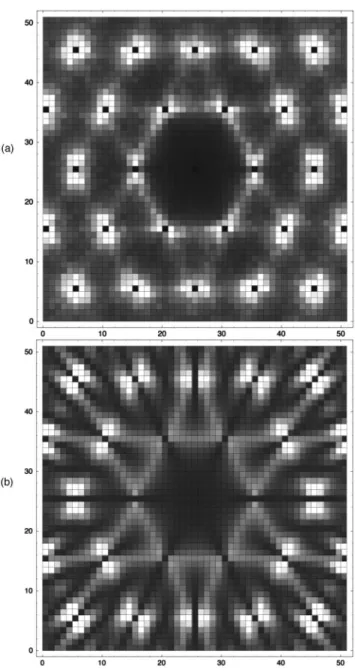
Now we compare our results with numerical simulation of the LLL system in Ref. 11. The general shape of the struc-ture function in the vicinity of a peak关see Fig. 1共b兲兴 and the data near the origin according to a MC simulation of the same system within the same LLL approximation in Ref. 11 关Fig. 1共a兲兴 are qualitatively the same pattern. It is easier to compare using rescaled quasimomenta, q→q

冑

b, k→k

冑

b. We get S共q,0兲⫽

冉

ah ␤A

冊

2 4␲2␦n共q兲 b exp

冋

⫺ q2 2

册

⫹ ␻ 2 a_h1/2 ␤A exp

冋

⫺q 2 2

册

⫻关 f1共q兲⫹␦n共q兲f2共Q兲⫹␦n共q兲f3兴, 共38兲 where f1(q), f2(Q), and f3are defined in Eq.共35兲, but with b⫽1 共for example, f₃⫽⫺28.5275) and the region of inte-gration in the formula rescaled to the cell with d˜1,d˜2 being the reciprocal lattice basis vectors

In Ref. 11, the material parameters describe YBCO: Tc ⫽93 K, dHc2(T)/dT⫽⫺1.8⫻104 Oe/K, ␥⫽5, and␬⫽52. At T⫽82.8 K, H⫽50 kOe. This leads to the following di-mensionless parameters Gi⫽2.04⫻10⫺5, ␻⫽0.056, a_h ⫽0.039 904. However, as discussed in Ref. 14 effective ex-pansion parameters are ah/6b⫽0. 222 68 and b␻(ah)⫺3/2/2

冑

2␲⫽2.36⫻10⫺2, both less than 1. ah/6b is the parameter for the expansion of the classical solution. The factor 6 comes from the fact that due to hexagonal, only 6th, 12th, etc. Landau levels appear in perturbation expansion. b␻(ah)⫺3/2/2

冑

2␲is the parameter for the fluctuation共loop兲 expansion and is much less than 1 here. It justifies the quan-tum correction of the formula using perturbation expansion. The numerical factor in front of the fluctuation correction in this case is

c1⫽

␤Ab␻共ah兲⫺3/2

8␲2 ⫽3.0932⫻10

(6)

In a finite size sample,␦n(q) is equal to LxLy/(2␲)2when q lies on the reciprocal lattice m1d˜1⫹m2˜d2; otherwise it is zero. Because LxLy⫽N␾2␲ (N␾ is the number of vortices of order 100 only in the MC simulation兲, it is equal to N_␾/2␲. The normalized structure function sn(0)⫽1, as it was used in Ref. 11兲 is

sn共q兲⫽⌬共q兲⫹ 1 共1⫹c1f3兲关 c2f1共q兲⫹c1⌬共q兲f2共Q兲兴共41兲 and c2⫽c1 2␲ N_␾⫽1.9435⫻10 ⫺4_, 1⫹c₁f₃⫽0.91315. 共42兲 The correction to the height of the peak at Q, c₁⌬(q)/关1 ⫹c1f3兴 f2(Q), is quite small. We find the height of the peaks away from the origin found in the MC simulation11are typi-cally smaller than ours, while around the peaks they are larger than analytical. It may be due to the finite size effect or finite samplings of the MC calculation. In the MC calcu-lation part of the peak might ‘‘belong’’ to a neighboring pixel. We plot the correction to the nonpeak region in Fig. 1共b兲 and find that the theoretical prediction has roughly the same characteristic saddle shape ‘‘halos’’ around the peaks as in Ref. 11, Fig. 1共a兲, in which all the peaks were removed 共so it is different from Fig. 2共a兲 in Ref. 11 in which only the central peak was removed兲.

We can extend our formula to higher orders which will include also the HLLs共higher Landau levels兲. To next order of ah, we should include ⌽1 in ⌽, ⌽⫽(ah)1/2关⌽0 ⫹ah⌽1兴, consider ⑀O(k),⑀A(k) to next order ah

2_{, and}

⑀O n

(k),⑀_An(k) to order ah. It is straightforward to do it.

B. Nonperturbative evidence of⑀_A1„k…˜円k円4

for asymptotic small kx,ky

Conversely, the MC simulation result provides the non-perturbative evidence ⑀_A1(k)→兩k兩4 _{for asymptotic small} kx,ky. In Eq.共36兲, if⑀A

_*_共x兲_␹_共x兲典 ⫹

具⌽共x兲

␹*共x兲

典⫹

具

␹共x兲␹*共x兲典

⫽ah

␤A兩␾共x兲兩

2_⫹

_具

_␹_共x兲_␹*_共x兲典_. _共43兲 FIG. 1. 共a兲 Structure factor from the MC simulation of Ref. 11.

The peaks at reciprocal lattice points are removed.共b兲 Fluctuation correction to structure factor of the Abrikosov vortex lattice, Eq. 共41兲. The peaks at reciprocal lattice points are removed.

TABLE I. Values of f2(Q) with small n1,n2.

n1,n2 0,1 1,0 1,1 1,2 0,2 2,2 1,3

(7)

Using Eq. 共20兲 and Eq. 共11兲, and considering only x3⫽0, one obtains

具

␹共x兲␹*共x兲典⫽ ␻ 16␲3

冕

k兩␸k共x兲兩 2

冋

1 ⑀O共k兲⫹ k₃2 2 ⫹ 1 ⑀A共k兲⫹ k₃2 2

册

⫽ ␻ 16␲2

冕

k兩␸k共x兲兩 2

冋

冑

2 ⑀O共k兲⫹

冑

2 ⑀A共k兲

册

.

However, as pointed out in Sec. III the coefficient ␯ in

␺(x)⫽v␾(x)⫹␹(x) is renormalized to one loop order, v2 ⫽vo

2_⫹_␻

v₁2, withv1 given in Eq.共33兲. Thus we need to add a term,␻v1 2_关_␾_(x)_兴2_{, to Eq.}_共43兲.

具

␳共x,0兲典⫽ah ␤A 兩␾共x兲兩2_⫹ ␻ 16␲2

冕

k兩␸k共x兲兩 2 ⫻

冋

冑

_⑀ 2 O共k兲 ⫹

冑

_⑀ 2 A共k兲

册

⫺␻兩␾共x兲兩 2 16␲2

冕

k

冋

冉

2␤_k⫹兩␥_k兩 ␤

冊

冑

2 ⑀O共k兲 ⫹

冉

冊

冑

2 ⑀A共k兲

册

. 共44兲

Its Fourier transform ␳(q)⬅兰dzeiq•z

具

␳(z,0)

典

can be easily calculated: ␳共q兲⫽4␲2_␦ n共q兲exp

冋

⫺ q2 4b⫹ iqxqy 2b ⫹ ␲i 2 共n1 2_⫺n 1兲

册

⫻

再

_␤ah A⫹ ␻ 16␲2

冕

k

⫺

冉

冊冊

冑

2 ⑀A共k兲

册

冎

. 共45兲

Performing integrals and rescaling the quasimomenta again, one obtains ␳共q兲⫽4␲2␦n共q兲 b exp

冋

⫺ q2 4 ⫹ iqxqy 2 ⫹ ␲i 2 共n1 2_⫺n 1兲

册

⫻

再

ah ␤A ⫹␻bah⫺1/2 16␲2 [⫺28.5275⫹ f2(Q)]

冎

. 共46兲 The function f₂(Q… appeared in Eq. 共36兲.

VI. DISORDER EFFECT ON MAGNETIZATION AND SPECIFIC HEAT

One can introduce weak disorder by adding a quadratic term in Eq. 共2兲,6

⌬ f ⬅

冕

d3_x_␣_共x兲兩_␺_兩2_. _共47兲 Loosely speaking it represents a local variation of tempera-ture. For pointlike defects one can assume that the correla-tion of␣(x) is

具具

␣(x)␣( y )

典典

⫽W␦(x⫺y),

具具

␣(x)

典典

⫽0. Be-fore the disorder average we calculate the free energy ⫺T ln Z with

Z⫽

冕

D␺*D␺exp

再

⫺ 1

␻

冋

f关␺*,␺兴⫺

冕

d3x␣共x兲兩␺兩2

册

冎

.

共48兲 If W is very small, we can calculate Z by perturbation theory in W. To the second order Z is given as

Z⫽Z0

冋

1⫺ 1

␻

冕

x␣共x兲具␳共x兲典 ⫹ 1

2␻2

冕

_x

冕

_y

具

␳共x兲␳共y兲典␣共x兲␣共y兲

册

典⫺具

␳共x兲典具␳共x兲

典兴

⫽F0⫺ TWV 2␻2 ␻S ˜_{f luct}_共0兲. _共51兲

From Eq. 共35兲, one finds that ˜S_{f luct}(0)⫽ ⫺0.186 19(ah

1/2_b/_␤

A). Hence the energy density difference due to disorder is F⫽⌬F/V⫽⫺0.0931(TWa_h1/2b/␻␤A). Since ␻⫽

冑

2 Gi␲2t,F⫽ca_h1/2b with c⫽ ⫺0.0931TcW/

冑

2 Gi␲2␤A. The disorder effect on magneti-zation and specific heat are

⌬m⫽⫺⳵_⳵⌬ f_b ⫽⫺c

冉

a_h1/2⫺b 4ah⫺1/2

冊

, 共52兲 ⌬c⫽⫺t⳵ 2 ⳵t2⌬ f ⫽ c 16tbah⫺3/2, respectively. VII. CONCLUSIONS

To conclude, we have calculated the effect of fluctuations on the structure function of the vortex lattice and compared it to existing MC results. In addition to renormalization of the height of the Bragg peaks, there appear characteristic saddle

(8)

shape ‘‘halos’’ around the peaks as found in Ref. 11. The MC simulation result provides the nonperturbative evidence

⑀A 1

(k)→兩k兩4 for asymptotic small k. The calculated fluctua-tion contribufluctua-tion to the magnetic field can be more easily observed in low temperature strongly type-II superconduct-ors. Finally, the predicted dependence of magnetization and specific heat on disorder via fluctuations also can be experi-mentally studied.

Correlations in flux lattices can be experimentally mea-sured using neutron scattering as well as some other more exotic methods such as muon spin relaxation, electron to-mography, scanning SQUID microscopy, etc.1–3,16,17 It would be interesting to detect the effect of fluctuations given in the present paper directly from experiments by subtracting the ‘‘background’’ of the well-known mean field correlator. The calculations show that infrared divergencies naively ex-pected in all of the physical quantities calculated above due to ‘‘supersoft’’ shear modes in the large␬ limit cancel. This strengthens the view that the loop expansion is a reliable theoretical tool to study the fluctuations effects in vortex lattice below the melting point.

ACKNOWLEDGMENTS

We are grateful to our colleagues A. Knigavko, B. Bako, and V. Yang. One of us 共B.R.兲 is especially grateful to R. Sasik and D. Stroud for providing raw numerical data which was essential for the present comparison with the MC data. The work is part of the NCTS topical program on vortices in high Tc and was supported by NSC of Taiwan.

APPENDIX A

In this appendix, we present some basic formulas used in the calculations. The basic matrix element is

b 2␲

冕

cell dx␸共x兲␸_k*共x兲exp关⫺ix•q兴 ⫽⌬q,kexp

冋

␲i 2 共n1 2_⫺n 1兲⫺ q2 4b⫺ iqxqy 2b ⫹ ikxqy b

册

. 共A1兲 The Kronecker delta is defined by

⌬q,k⫽⌬共q⫺k兲⫽

再

1, if q⫽k⫹n1d˜1⫹n2d˜2

0, otherwise, 共A2兲 where integers n1⫽(1/2␲)d1•(q⫺k) and

n2⫽共1/2␲兲d2•共q⫺k兲.

Here d˜₁,d˜₂ are the reciprocal lattice basis vectors

1_{P. L. Gammel et al., Phys. Rev. Lett. 68, 3343}_共1992兲. 2_{B. Keimer et al., Phys. Rev. Lett. 73, 3459}_共1994兲. 3_{I. Maggio-Aprile et al., Phys. Rev. Lett. 75, 2754}_共1995兲. 4

E. Zeldov, D. Majer, M. Konczykowski, V. B. Geshkenbein, V. M. Vinokur, and H. Shtrikman, Nature 共London兲 375, 373 共1995兲.

5_{D. R. Nelson, Phys. Rev. Lett. 60, 1973}_共1988兲.

6_{G. Blatter, M. V. Feigel’man, V. B. Geshkenbein, A. I. Larkin,}

and V. M. Vinokur, Rev. Mod. Phys. 66, 1125共1994兲.

7_{M. Tinkham, Introduction to Superconductivity} _{共McGraw-Hill,}

New York, 1996兲.

8_{G. Eilenberger, Phys. Rev. 164, 628} _{共1967兲; K. Maki and H.}

Takayama, Prog. Theor. Phys. 46, 1651共1971兲.

9_{A. Ikeda, T. Ohmi, and T. Tsuneto, J. Phys. Soc. Jpn. 59, 1740}

共1990兲; 61, 254 共1992兲; A. Ikeda, ibid. 64, 1683 共1994兲; 64, 3925共1995兲.

10_{M. A. Moore, Phys. Rev. B 39, 136}_{共1989兲; 45, 7336 共1992兲.} 11_{R. Sasik and D. Stroud, Phys. Rev. Lett. 75, 2582}_共1995兲. 12_{G. J. Ruggeri, Phys. Rev. B 20, 3626}_共1978兲.

13_{B. Rosenstein, Phys. Rev. B 60, 4268}_共1999兲.

14_{D. Li and B. Rosenstein, Phys. Rev. B 60, 9704}_共1999兲. 15_{I. Affleck and E. Brezin, Nucl. Phys. B 257, 451}_共1985兲. 16_{R. Cubitt et al., Nature}_{共London兲 365, 407 共1993兲.}

17_{L. N. Vu, M. S. Vistrom, and D. J. Van Harlingen, Appl. Phys.}

Thermal fluctuations and disorder effects in vortex lattices

Thermal fluctuations and disorder effects in vortex lattices

冕

冏

冉

冊

冏

⬘

冑

⬘

冕

冋

册

冑

具兩

典

冑

冑

兺

冉

冑

冊

再

冋

冑

册

冉

冑

冊

冎

冑

冑

冑

冑

兺

冑

冑

兺

冉

冑

冑

冊

再

冋

冉

冑

冑

冊

册

冉

冑

冑

冊

冎

冑

冕

冑

兺

冑

冑

冕

冑

兺

冑

冉

冊

冉

冊

具

典

具

典

具共

典

具

典

具 典

具 典

具兩⌽共x兲兩

典

_冑

_具

_具

_典

_具共

_具

具典

具典

_典兲e

_典⫽

_典