基於圖形處理器之即時熱影像模擬

國

立

交

通

大

學

多媒體工程研究所

碩 士 論 文

基於圖形處理器之即時熱影像模擬

GPU-based Real-Time Simulation of Thermogrphy

研 究 生：邱晟瑋

指導教授：林奕成 博士

基於圖形處理器之即時熱影像模擬

GPU-based Real-Time Simulation of Thermogrphy

研 究 生：邱晟瑋

指導教授：林奕成

Student：Cheng-Wei Chiu

Advisor：Dr. I-Chen Lin

國 立 交 通 大 學

多 媒 體 工 程 研 究 所

碩 士 論 文

A Thesis

Submitted to Institute of Multimedia Engineering College of Computer Science

National Chiao Tung University in partial Fulfillment of the Requirements

for the Degree of Master

in

Computer Science

July 2010

Hsinchu, Taiwan, Republic of China

I

基於圖形處理器之即時熱影像模擬

研究生：邱晟瑋 指導教授：林奕成 博士

國立交通大學

多媒體工程研究所

摘要

II

GPU-based Real-time Simulation of Thermography

Student: Cheng-Wei Chiu

Advisor: Dr. I-Chen Lin

Institute of Multimedia Engineering

National Chiao Tung University

Abstract

The goal of this thesis is to propose an efficient framework for real-time thermography

simulation. Since our purpose is not fully physical simulation but visually correct

thermographic view, we propose a plausible illumination method for approximation of heat

transfer where radiation, conduction and convection are all included. We use Phong

illumination model to simulate radiation since indirect reflection can be ignored with low

temperature difference. For simulation of conduction, we construct less 2D textures to

substitute a large-sized volumetric 3D object to reduce computational complexity of heat

propagation. To simulate convectional effect, we simplify the shapes of objects into

cylindrical case and apply the formula of heat transfer from a cylinder in cross flow. All of

these methods are able to be accelerated by GPU-based rendering which synthesizes realistic

thermal images of a virtual environment in real-time.

III

Acknowledge

First of all, I would like to thank my advisor, Dr. I-Chen Lin, for his guidance in the past two

years. Also, I appreciate all members of Computer Animation & Interactive Graphics Lab for

IV

Contents

1. Introduction ... 1 1.1 Motivation ... 1 1.2 Background ... 3 1.3 Framework ... 7 2. Related Work ... 9 3. Overview ... 12 4. Voxelization of 3D Model ... 14 4.1 GPU-Based Voxelization ... 14

4.2 Optimization of Voxelized Texture ... 17

4.3 Multi-Level Voxelized Texture ... 20

5. Simulation of Heat Transfer ... 22

5.1 Radiation from Heat Source ... 22

5.2 Heat Propagation ... 25

5.3 Conduction by Contact ... 27

5.4 Convection in Cylinder Case ... 30

6. Experiment Results ... 33

6.1 The Analysis of Voxelized Structure ... 33

6.2 Turbulent Flow Effect in Convection ... 37

6.3 System Performance ... 40

7. Conclusion ... 43

V

List of Figure

Figure 1.1 Normal visions and thermal images. (a) Through smoke in daylight. (b) Through foliage in daylight. (c) Through shadow at night [PR]. ... 2 Figure 1.2 Thermal image of houses which display heat radiation in color and

black-and-white [Thermal Image]. ... 2 Figure 1.3 Radiosity method using in global illumination [PCG]. ... 4 Figure 1.4 Image-based algorithms, Screen Space Ambient Occlusion (SSAO) and Directional Occlusion (SSDO) [Mitt07, RGS09]. ... 4 Figure 1.5 Thermal image of hand print on wall [PR]. ... 5 Figure 1.6 Thermal image of heat loss around windows by thermal convection. ... 6 Figure 1.7 Visual simulation of thermal fluid dynamics in a pressurized water reactor

[FKZQ*09]... 7 Figure 1.8 The flow chart of the proposed system of synthesis thermal images. ... 8 Figure 2.1 The synthesis procedure of infrared targets and the background [WWBP01]. ... 9 Figure 2.2 The mesh used to incorporate a complex conduction environment and the result of

stimulation [HPH00]. ... 10 Figure 2.3 Particles advected in a 2D flow field based on the D2Q9 LBM model [LWK03]. 11 Figure 4.1 From left to right: mesh of penguin, large voxel size and small voxel size voxelized

model by slice method. The smaller voxel size results more precise shape of mesh and more storage data used. ... 14 Figure 4.2 The flow chart of GPU-based voxelization algorithm. ... 15 Figure 4. 3 Voxelized textures of “Happy Buddha”. There are 18 layers in x axis, 20 in y and 8 in z; the left shows depth value in the first three textures of z axis. ... 16 Figure 4.4 The first layer images from orthogonal view on X and Z axis overlap on cross area.

... 17 Figure 4.5 Voxelized texture of sphere rendered from x axis: (a) depth value; (b) normal of

surface; (c) repainting red on fragment if ∥nx∥ is greatest, green for y axis and

blue for z; (d) preserved area of (c). ... 18 Figure 4 6 Voxelized texture of “Happy Buddha” rendered from z axis with surface normal,

from left to right: (a) original, (b) stored and (c) packed texture. After packing, the number of layers in x is 8, 11 in y and 6 in z axis. ... 19

VI

Figure 4.7 The example of optimization of voxelized texture. ... 20 Figure 4.8 Voxelized texture of sphere slice. From left to right is single shell, multi-level and

irregular multi-level. The irregular multi-level varies voxel size with different levels. Because of overlap occurring on some voxels, the conduction weight between voxels should be adjusted. ... 20 Figure 5.1 Four styles of voxelization: (a) full volume, (b) single shell, (c) multi-level and (d)

irregular multi-level. Red lines are shown the shortest heat flux paths form right to left side. ... 25 Figure 5.2 Heat propagation of “Happy Buddha” from left to right are single shell, multi-level and full volume, with each time steps: (a) 30s, (b) 60s, (c) 90s and (d) 180s. ... 26 Figure 5.3 Intersection volume at different resolutions. Left: the collision surfaces. Middle:

the intersection volume at resolution 16×16. Red, green and blue pixel show the bounds in x,y and z directions, respectively. Right: resolution 256×256. [FBAF08] ... 27 Figure 5.4 The example of two cylinders contact. We render B on bounding box of A in Z axis

and apply depth peeling. Voxelized texture of A replaces depth buffer in peeling process. The texture TA records contact area on surface of A. ... 28

Figure 5.5 The contact of a hat ball and cool Planck’s head. The collision area occurs on top of head which is corresponding voxelized texture (a). (b) shows the conduction texture THead, which records energy of ball at contact. This energy conducts to (a)

immediately and heat voxelized texture as (c) shown. The bottom of ball and the top of head conduct and spread the heat after 2 second, and we get the conduction texture THead as (d), voxelized texture as (e). ... 29

Figure 5.6 Local Nusselt number for airflow normal to a circular cylinder. [ IDBL*06] ... 31 Figure 5.7 The velocity of cross-flow in circular cylinder shows turbulent flow. The dark color represents low velocity, and bright color represents high velocity in flow. ... 32 Figure 5.8 The variation of temperature with heat convection as time passes by. ... 32 Figure 6.1 The Conduction of “Happy Buddha” with multi-level structure, each row

represents the variation of three directions with four different settings through 3600 iterations. There are single shell, 10 levels, 100 levels and full volume structure from the left to the right hand side in a single image. ... 34 Figure 6.2 The contact area between different levels occur crack or overlap when the model is

VII

Figure 6.3 The conduction result of irregular multi- level structure and full volume, each row represents the variation of three directions through 4000 iterations. ... 36 Figure 6.4 Wind flow simulation by LBM with different pipe diameter 800×300 and 800×600. (a) and (c) show fully developed flow. (b) and (d) show average velocity. ... 37 Figure 6.5 The average velocity distribution with distance from the object is represent as a .. 38 Figure 6.6 The cylinder low by LBM method with different wind speed, (a) 1.0, (b) 0.8, (c)

0.4 and (d) 0.2 m/s. ... 39 Figure 6.7 The normalized average velocity from Figure 6.3 with distance varying. ... 39 Figure 6.8 The simulation time of conduction in “Happy Buddha”. ... 41 Figure 6.9 The voxel number compression rate of texture-based method, single shell and

irregular multi-level, in “Happy Buddha” case. ... 41 Figure 6. 10 The simulation time of conduction in “Max Planck”. ... 42 Figure 6.11 The voxel number compression rate of texture-based method in “Max Planck”

VIII

List of Table

Table 1.1 Comparison between traditional graphics and infrared images. ... 3 Table 5.1 The variations of temperature by fully absorbing 31.15Wm-2 on 1m3 cube. ... 23 Table 6.1 “Happy Buddha” model in four voxelized structure type with225×550×225 volume

1

1. Introduction

1.1 Motivation

To acquire more clear images from dim or dark environment, we have to utilize specific

sensors to enhance dim images or visualize signals besides visible light spectrums. Thermal

image device is the one of most pervasively used sensor for such purposes in military or

secure usages.

Thermography is a type of infrared imaging science. Thermographic cameras detect radiation

in the infrared range of the electromagnetic spectrum and visualize the received radiation.

Since infrared radiation is emitted by all objects, according to the black body radiation law,

thermography allows one to see variations in temperature. When viewed by a thermographic

camera, warm objects are much more conspicuous than cooler backgrounds. Therefore,

humans and other warm-blooded animals become easily visible against the environment, in

either day or night. As a result, thermography are extensive used for uncover humans or

vehicles in military or security purposes. Besides, it is also helpful for other usages. For

instance, firefighters use it to see through smoke, find persons, and localize the base of a fire.

With thermal imaging, power-lines-maintenance technicians locate overheating joints and

parts, a sign of their failure, to avoid potential hazards.

However, it is expensive and risky to train novices in invisible environments. One of the

practical substitutions is training the novices in a virtual environment where thermography is

simulated. This environment is controllable to decrease danger and costly hardware; it also

2

The goal of this thesis is to propose an efficient framework for real-time thermography

simulation. Since the views of environments by thermograhpic camera are due to variations in

temperature, we simulate the heat transfer system to visualize temperature information from

synthetic environments, which includes a plausible illumination model for approximation of

physical heat transfer. While completely performing the detail of theory of heat transfer is

computationally intensive, the goal of this simulation focus on rendering visually realistic

thermal images instead of exactly implementing all the formulas of heat transfer system.

(a) (b) (c)

Figure 1.1 Normal visions and thermal images. (a) Through smoke in daylight. (b) Through foliage in daylight. (c) Through shadow at night [PR].

Figure 1.2 Thermal image of houses which display heat radiation in color and black-and-white [Thermal Image].

3

1.2 Background

When an object or fluid is at a different temperature from its surroundings, transfer of thermal

energy, also known as heat transfer, or heat exchange, occurs in such a way that the body and

the surroundings gradually reach thermal equilibrium. Heat transfer always occurs from a

higher-temperature object to a cooler-temperature one as described by the second law of

thermodynamics. Where there is a temperature difference between objects in proximity, heat

transfer between them can never be stopped; it can only be slowed. In this simulation system,

all methods of heat transfer also repeatedly calculate the variation of heat. The heat transfer

methods comprise three types of phenomena: radiation, conduction and convection.

Radiation:

All objects with a temperature above the absolute zero radiate energy at a rate equal to their

emissivity multiplied by the rate at which energy would radiate from them if they were a

black body. No medium is necessary for radiation to occur, since it is transferred through

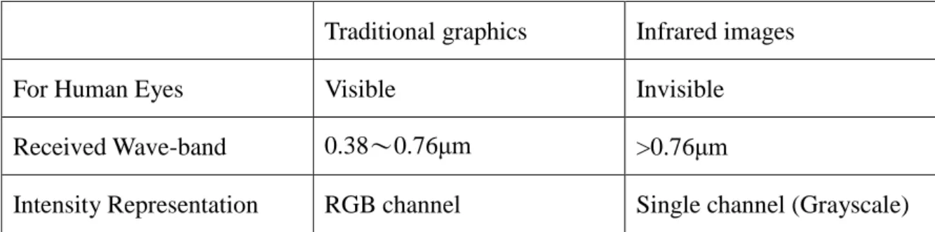
electromagnetic waves. By comparing traditional graphics and infrared image shown as Table

1.1, we know that the critical difference is range of wave-band. If we replace reflection

coefficients by thermal reflection coefficients in traditional graphics rendering, we can get

same result of thermal image.

Table 1.1 Comparison between traditional graphics and infrared images. Traditional graphics Infrared images

For Human Eyes Visible Invisible

Received Wave-band 0.38〜0.76μm >0.76μm

4

The radiosity [GTGB84] method is used to solve for the radiative heat transfer between

numbers of surfaces. This method is also applied in 3D computer graphics for global

illumination rendering. Vice versa, these algorithms of global illumination [Land02, ZIK98,

Bunn05] can solve for the radiative heat transfer as well. However, most radiosity-based

algorithms make use of iterative light transfer calculations which is of high computation cost.

On the other hand image-space algorithms [DS05, Mitt07 and RGS09] can be an efficient

approximation of global illumination. Though these approximation methods are of high

computational efficiency, it may not provide all required effects.

Figure 1.3 Radiosity method using in global illumination [PCG].

Figure 1.4 Image-based algorithms, Screen Space Ambient Occlusion (SSAO) and Directional Occlusion (SSDO) [Mitt07, RGS09].

5

Conduction:

Conduction is the transfer of heat from one molecule of matter to another. Conduction is

greater in solids, where atoms are in constant contact. In liquids (except liquid metals) and

gases, the molecules are usually further apart, giving a lower chance of molecules colliding

and passing on thermal energy.

Figure 1.5 Thermal image of hand print on wall [PR].

To simulate the conduction phenomena, molecular dynamic (MD) methods are generally

accepted means for simulating molecular scale models of matter. Objects and time step of

simulation should be divided as tiny as well to describe the technique as a “virtual microscope”

with high temporal and spatial resolution. Besides, conduction between dynamic objects

should consider whether there’re surface contacts. That means the relation of connection

changed during the movements in scene. There are two main categories of collision detection,

object-based [KHMS*98] and image-space-based [BWS99] algorithm. The object-based

collision detection computes the bounding volumes of objects in 3D scene. The image-based

collision detection only computes the data of rendered images (e.g. depth value or color

value). The weakness of object-based collision detection is its computational complexity.

When complexity of the scene is complicated, the computing time will increase since our

6

Convection:

Convection is the movement of molecules within fluids (i.e. liquids and gases). As the fluid

moves quicker, the convective heat transfer increases. Nevertheless, the presence of bulk

motion of the fluid also enhances the heat transfer between the solid surface and the fluid. For

example, an ice cube melts faster when it is blown in the wind.

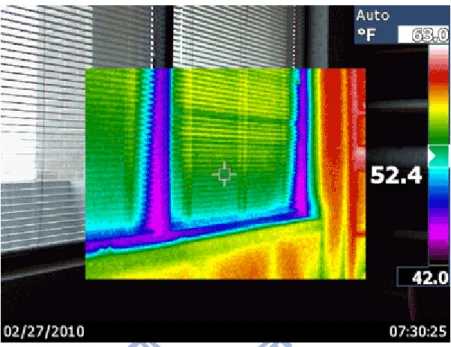
Figure 1.6 Thermal image of heat loss around windows by thermal convection.

According to the definition of computational fluid dynamics (CFD), numerical methods can

be used to solve and analyze problems that involve fluid flows. While apply full CFD for

convection, it requires the millions of calculations to simulate the interaction of liquids and

gases with surfaces defined by boundary conditions. Lattice Boltzmann method (LBM) is a

class of CFD methods for fluid simulation. It solves the conservation equations of

macroscopic properties numerically unlike the traditional CFD methods. LBM models the

fluid consisting of fictive particles which perform consecutive propagation and collision

processes over a discrete lattice mesh. Due to its particulate characteristic, LBM takes

7

and parallelization of the algorithm. However, this method does not support simulating

incompressible flow such as gas and high-speed fluid.

Figure 1.7 Visual simulation of thermal fluid dynamics in a pressurized water reactor [FKZQ*09].

1.3 Framework

In this thesis, we present an approximation of heat transfer system which consists of radiation,

conduction, convection and producing visually similar thermal image. The process includes

two main steps:

1. Voxelization for 3D Model. Since the temperatures between various parts of object may

not be the same, we use the finite element method to visualize temperature of object in

detail. For this purpose, we separate surface of object model in orthogonal views and store

geometric information to a series of textures. By this step, an object model can be

represented as numerous voxels.

2. Simulation of Heat Transfer. Voxelized objects exchange heat with other voxels in

8

equilibrium of objects and environment. The voxelization textures store heat energy and

update in parallel through GPU calculation. Finally, we render objects with stored heat in

textures and reflected heat of radiation on surface in screen.

To make our simulation efficient, we propose a GPU-liable visualization system. All of these methods are able to be accelerated by GPU-based rendering which synthesizes realistic

thermal images of a virtual environment in real-time.

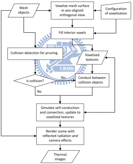
Figure 1.8 The flow chart of the proposed system of synthesis thermal images. Voxelize mesh surface

in axis-aligned orthogonal view

Fill interior voxels

Configuration of voxelization

Collision detection for pruning

Is collision? Conduct between _{collision objects}

Simulate self-conduction and convection, update to

voxelized textures Yes

No

Render scene with reflected radiation and

camera effects Voxelized textures Mesh objects Thermal images

9

2. Related Work

Infrared Image Synthesis. C. Garnier et al. [GCFM*99] described an IR sensor model

developed from study of physical effects involved in IR image acquisition process. Their

approach consists of a combination and an extension of current camera models used in visible

and infrared image synthesis, and they also merges ray tracing and post-processing techniques.

Zhangye Wang et al. [WWBP01] established an infrared model for ground targets, such as

tank. They considered the effect of inner heat source, friction and various environmental

factors and drew infrared images of target at various states by the Computer Graphics

techniques. Zhangye Wang et al. [WPLJ01] and Zhaoyi Jiang et al. [JWJP04] proposed new

IR image synthesis model accounting for meteorological, environmental, material and

artificial factors. The energy equilibrium equation is built based on the principle of heat

transfer and infrared physics and a finite difference method is adopted to solve the equations.

Zhaoyi Jiang et al. [JWP03] proposed a method to constitute the dynamic infrared scene by

combining scene geometric modeling with multi-spectral image. Multi-spectral IR textures

are correspondent to materials of object surface. The actual attenuated IR radiation intensity is

expressed by Phong illumination model between 10℃and 50℃.

10

Molecular Dynamic for Conduction. Molecular dynamic (MD) methods are now generally

accepted approaches for simulating molecular scale models of matter. The essence of MD

simulation methods is simply stated: numerically solve the N-body problem of classical

mechanics. H. Xue and C. Shu [XS99] presented investigation to deals with the equilibration

of heat conduction simulation in a very thin film using MD. David M. Harrild et al. [HPH00]

described the novel application of a Finite Volume method (FVM) derived from

computational fluid dynamics to the field of computational cardiac electrophysiology. They

applied this method to simulate conduction in an arbitrarily shaped or complex region.

Jiaocheng Ma et al. [MXJ08] proposed real-time mathematical 2D heat transfer and

solidification model. This model was presented for billet continuous casting of low carbon

steel and solved by FVM. The GPU-based implementation is faster than that of CPU-based

MD simulation. Juekuan Yang et al. [YWC07] presented an implementation of MD

simulation on modern graphics processing units (GPU). This GPU algorithm was used to

calculate the thermal conductivities of solid argon and to reduce the total computational time

of conduction simulation at high performance. These methods mentioned above are used to

analyze and solve heat flux propagation on a single solid object but they are difficult to

represent interaction with other objects.

Figure 2.2 The mesh used to incorporate a complex conduction environment and the result of stimulation [HPH00].

11

Fluid dynamic. The solution to a fluid dynamics problem typically involves calculating

various properties of the fluid, such as velocity, pressure, density, and temperature, as

functions of space and time. Wei Li et al. [LWK03] presented a physically-based flow

simulation which supports complex boundary conditions running on the general-purpose

graphics hardware. For computing the flow field, they accelerated the computation of the

Lattice Boltzmann Method (LBM) on GPU, by grouping particle packets into 2D textures and

mapping the Boltzmann equations completely to the rasterization and frame buffer operations.

To handle complex, moving and deformable boundaries, they proposed a generic voxelization

algorithm of the boundaries using depth peeling, and extended it to a dynamic boundary

generation method that converts any geometric boundary to LBM boundary nodes on-the-fly.

Zhe Fan et al. [FKZQ*09] presented a simulation and visualization system for the thermal

fluid dynamics inside a pressurized water reactor of a nuclear power plant when cold water is

injected into the reactor vessel. They employed a hybrid thermal lattice Boltzmann method,

which has the advantages of ease of parallelization and ease of handling complex simulation

boundaries.

12

3. Overview

In this chapter, we will briefly describe our method and each chapter afterward.

We propose our voxelization algorithm in chapter 4. The energy of molecules on object

surface may not be the same in dynamic state of heat transfer. The objects in simulation

should be divided into voxels as tiny as well. We generate voxelized textures from objects by

depth peeling in axis-aligned orthogonal views. These textures which stored energy and

geometrical information are able to compute variation of heat in parallel through GPU. Since

the method is only valid to surfaces, we fill the voxels in multiple layered textures with large

weight of heat capacity for simulating volume of object. By comparing with full volume

resolution, our methods compress voxel number into 10~25%.

Chapter 5 includes the details of heat transfer simulating. In order to rapidly generate visually

reasonable scene in simulation of radiation, we ignore the interactive reflection between

objects with low temperature difference. We implement shadow map and Phong shading

model while low intensity heat source. In addition, screen space ambient occlusion (SSAO)

[Mitt07, RGS09] is used to enhance detail in high temperature difference.

To simulate conduction, we separate the render pass into pruning, contact detection and

spreading phases. First, we use the linear-time CULLIDE [GRLM03] algorithm to prune

collision-free objects in image space which are unnecessary for computation of heat exchange.

Once a collision is detected, the contact surfaces make heat pass through from hot to cool side.

We apply Layered Depth Images (LDI) extended method [FBAF08] which processes contacts

13

spreads heat through itself until the distribution of heat is equilibrium.

Computation with computational fluid dynamics (CFD) usually involves intensive

computation in general convection processing. Due to our real-time and visually acceptable

requirement, we represent the shape of object by combination of cylinders. Heat transfer

between fluid and such simple shape can get approximate distribution [BJO98, KCY06]. By

appling this approximation we can speed up the calculation between surface and fluid from

O(n3) to O(n2logn) which n defined boundary of the scene.

Our experiment and result are presented in chapter 6. According to performance and visual

result, we provide optimal parameters for this simulation system. At last, we summarize our

14

4. Voxelization of 3D Model

Since the temperatures between various parts of an object may not be the same, we should

divide the object into regular volumes, so called voxels, with its own thermal energy for

simulating heat transfer in dynamic state. A voxel is a volume element, comprising a value on

the regular grid in three dimensional space. In our system, the variations of temperatures on

object surfaces are displayed by voxels in continuous domain.

4.1 GPU-Based Voxelization

Figure 4.1 From left to right: mesh of penguin, large voxel size and small voxel size voxelized model by slice method. The smaller voxel size results more precise shape of mesh and more storage data used.

An intuitive voxelization approach is the slicing method [FC00]. This method sets distance of

near and far clips planes as a single voxel size and renders only the geometry falling into the

slab between the two clip planes. The clip planes are shifted to generate subsequent slices

until entire volume covered with these slices. Our simulation method mostly interacts around

surfaces of objects which are sparse in a volume slice in most case. In other words, only a

small percentage of voxels are intersected by the boundary surfaces. There is no need to

15

heat spreading involves interior volume and we present how we reduce the amount of voxel

and keep visually-similar approximation in chapter 4.3.

Figure 4.2 The flow chart of GPU-based voxelization algorithm.

The GPU-based voxelization algorithm we used is the method proposed by Wei Li et al.

[LFWK03]. They avoid a slicing method by the idea of depth peeling [Ever01] used for

order-independent transparency. The depth layers in the scene are stripped away with

successive rendering passes. The procedure can be divided into three steps:

1. At first, the scene is rendered normally and the layer of nearest fragments as voxels is

obtained. During the second rendering pass, each fragment compares depth value with the

depth texture obtained from the depth buffer of the previous pass.

True Mesh Data Depth peeling Occlusion Query Voxelized Texture End state False

16

2. The fragment is discarded if either depth test is not pass or depth value greater than that

depth texture.

3. The process continues until no fragment is farther away than the corresponding pixel in

the depth texture. This condition is best determined by using a hardware occlusion query,

which returns the number of pixels written to the frame buffer.

We apply the peeling process three times. Each time, the image plane is orthogonal to one of

the major axes. The viewport is translated so that the layer images do not missing voxels but

are tiled as tightly as possible.

Figure 4. 3 Voxelized textures of “Happy Buddha”. There are 18 layers in x axis, 20 in y and 8 in z; the left shows depth value in the first three textures of z axis.

We apply depth peeling and save layer images with depth value in textures named voxelized

texture. There are three series of voxel data from each orthogonal view in these textures as

shown in Figure 4.3. The 3D position of voxel can be restored as texture coordinate and depth

in voxelized texture. As a result of peeling from three orthogonal views, some of the voxels

may be rendered more than once. The replication does not affect the accuracy but we can

reduce it to save more space and computing times.

Y Axis

Z Axis

17

4.2 Optimization of Voxelized Texture

We get voxelized textures by three-view depth peeling algorithm but these voxelized texture

data can further be optimized for acceleration of simulation system.

The improvement mainly occurs at overlapping areas in voxelized textures if the areas can be

rendered from two or three orthogonal views. We take a sphere for example. Figure 4.4 shows

the first voxelized textures from x and z axis. These textures which are rendered as

hemisphere of the sphere overlap at the same quarter with another one. Though all voxels are

unique in single orthogonal view, the same area may be rendered repeatedly by each peeling

process in the worst case. That means we may simulate on the same voxel twice or more but it

is not necessary. Therefore, we should store each voxel only once in all voxelized textures.

Figure 4.4 The first layer images from orthogonal view on X and Z axis overlap on cross area.

To keep the structure of voxel integrity, stored areas in each axis-aligned texture must be

independent of other orthogonal views. Then, we consider the attribute of surface normal to

check each fragment on voxelized texture whether the absolute normal weight of view axis is

greater than other two axes. For instance, if n is normal vector of surface and absolute normal

X Axis Z Axis

Overlapping Area

18

weight of x-axis ∥nx∥ is greater than ∥ny∥ and ∥nz∥, the corresponding fragment is

preserved as a voxel in x-axis peeling process.

(a) (b) (c) (d)

Figure 4.5 Voxelized texture of sphere rendered from x axis: (a) depth value; (b) normal of surface; (c) repainting red on fragment if ∥nx∥ is greatest, green for y axis and blue for z;

(d) preserved area of (c).

After removing replication of voxelized textures, more empty space may be generated due to

image space quantization at view change. As shown in Figure 4.6 (a) and (b), some of these

textures contain only few voxels or completely empty. We pack texels to fill empty space

before its texture as forward as possible and remove textures without any voxel data. Through

packing textures process, the number of layers is decreased which affects the number of

simulation computing times. We compare the textures of “Happy Buddha” with/without data

packing. The number of layers decreases to a half.

The last step of optimization is to build connection of voxels. We do not know whether these

voxels connect others around after packing. Even though we can find the connection by

restored 3D position of voxels, it has to be precomputed to reduce traversal neighbor texels

19 (a) (b) (c)

Figure 4 6 Voxelized texture of “Happy Buddha” rendered from z axis with surface normal, from left to right: (a) original, (b) stored and (c) packed texture. After packing, the number of layers in x is 8, 11 in y and 6 in z axis.

We summarize the procedure of optimizing voxelized textures. First we remove the replicate

voxels by comparing absolute normal weight of orthogonal axis. The voxels with maximum

absolute normal weight in viewing axis should be preserved. We pack the preserved voxels as

forward as possible in voxelized textures for fill the empty spaces. After packing, we reduce

the layer if layer of texture is completely empty. At last step we reconstruct the connection of

voxels and save connecting information in corresponding textures. Figure 4.7 represents the

20

Figure 4.7 The example of optimization of voxelized texture.

4.3 Multi-Level Voxelized Texture

Our voxelization algorithm generates only a single shell of target model. However, not all of

objects fit in this case; it may be solid or more complicated structure inside. We will deal with

solid and uniform material for conduction simulating. For this reason, we build voxelized

textures inside the shell.

Figure 4.8 Voxelized texture of sphere slice. From left to right is single shell, multi-level and irregular multi-level. The irregular multi-level varies voxel size with different levels. Because of overlap occurring on some voxels, the conduction weight between voxels should be adjusted.

We can build inner textures easily from original object and shell textures. If we construct all Level 1 Level 2 Level 3 Level 4 Empty Texel Layer 1 Layer 2 Layer 3 Removing

21

voxels inside of object with the same size of shell voxels, the number of textures explosively

increases and it cannot take our advantage of acceleration anymore. The voxels inside should

be considered with larger capacity than those outside, and then we only need to build fewer

textures for interior voxels.

We use a half resolution to record interior voxel data. Such as mipmap texture, each level

means one more layer inside and texture size smaller than level before. Figure 4.8 shows the

voxelized texture of sphere slice by single shell, multi-level and irregular multi-level. The

voxel size is presented as conduction weight between different levels of textures in simulation.

Besides, we must be careful about increasing voxel size, and total capacity must be kept in

original volume. We discuss multi-level and irregular multi-level structure in chapter 5 and 6

in detail.

We construct multi-level structure on full volume voxel data but our voxelized texture. Since

adding one level means to add the same size of our voxelized texture, it is difficult to divide a

large amount of voxels inside into three axis-aligned textures. However, we can build the

irregular multi-level structure in voxelized texture. There are few irregular voxels inside

22

5. Simulation of Heat Transfer

5.1 Radiation from Heat Source

According to Stefan–Boltzmann law, the power emitted per unit area of the surface of a black

body is directly proportional to the fourth power of its absolute temperature. That is

𝑞

_{= 𝜎𝜀𝑇}

₍₁₎

Where q” is the total power radiated per unit area, T is the temperature in the Kelvin scale, ε

is the thermal emissivity and σ = 5.67×10−8W·m−2·K−4 is the Stefan–Boltzmann constant. It

means that anything emits thermal radiation if it is higher than absolute zero in temperature.

Besides, thermal radiation may be absorbed, reflected or transmitted. It is difficult to apply

radiosity algorithm with each feature in real-time. For the reason, we approximate parts of

processes of total radiation and simulation with the following assumptions.

At first, the heat source, such as the sun, emits thermal energy to the scene. In general case,

the environment temperature is about 300K and the sun is about 5800K. During the daytime,

the sun emit energy about 1000W·m-2 to Earth. In contract, the energy emits from other object

can usually be omitted because of low temperature difference. We assume the max

temperature difference in the scene to be 100K, if there is no additional heat source, and the

max radiation is about 31.15W·m-2(distance between objects: 10m). We project this energy to

cubes with different materials whose volume is 1m3 and assume cubes absorbing energy fully

as black body. The variations of temperature are shown as Table 5.1. Actually, these materials

23

As this result, we only calculate radiation from heat source to the scene but from other

objects.

Table 5.1 The variations of temperature by fully absorbing 31.15Wm-2 on 1m3 cube.

Material Density kg/m3 Heat Capacity(25℃)

J/(kg·K) ΔT K·s-1 Platinum 21.45×103 135 _1.08×10-5 Gold 19.3×103 126 _1.28×10-5 Mercury 13.58×103 140 _1.64×10-5 Lead 11.34×103 128 2.15×10-5 Silver 10.49×103 233 _1.27×10-5 Copper 8.96×103 386 _9.01×10-6 Iron 7.87×103 444 _8.91×10-6 Diamond 3.5×103 509.1 1.75×10-5 Aluminum 2.7×103 897 _1.29×10-5 Water 1×103 4186 _7.44×10-6 Alcohol 0.79×103 2440 _1.62×10-5 Gasoline 0.73×103 2220 1.92×10-5

Since the reflection term is based on intensity of heat source but variation of temperature, it

cannot simplify as emission. At assumption of the radiation under a single wavelength,

objects between Ai and Aj, the intensity of radiation from patch dAi to dAj is:

dqi→j = Ii cosθi dAi

dAjcosθj

Rij2

24

Ii is the intensity of Ai, θi andθj is included angles between 𝑑𝐴 and normal of patches 𝑖𝑑𝐴𝑗

and Rij is length between dAi and dAj. If the distance is too far from heat source to object

surface or heat source is very small as a point, such as the sun, the intensity of radiation can

be formed as the diffuse term in Phong reflection model.

I

= k

(L∙N)i

(3)

kd is diffuse reflection constant, L is the direction vector from the point on the surface toward

each light source, N is the normal at this point on the surface and id is intensity of light source.

The ambient term in Phong model is to simulate accumulated inter-reflection in the scene but

it is unidirectional and too rough for complicated scene. The reflection of radiation is similar

with global illumination which contains direct and indirect light computing. We can get the

first reflection from heat source easily but it’s costly to compute indirect reflection repeatedly

until thermal equilibrium. For simulating dynamic scene in real-time, we use Phong model

and shadow map to render direct light and ambient occlusion map to approximate indirect

light if the scene is complicated.

We assume that all materials in the scene are opacity to simplify the problem. For these

assumptions, we only deal with emission and reflection of radiation from heat source as the

scene by using Phong model and shadow map, optional indirect reflection by ambient

occlusion if the scene is complicated. We render the emission of heat source to voxelized

textures represented each object in the scene. The reflection is rendered in screen

25

5.2 Heat Propagation

The area irradiated by heat source gains energy and the heat is propagated in the whole solid

object until energy balance. In each rendering pass, we spread the energy of voxels to

connected neighbor for each voxelized texture.

𝑞 = 𝑘 ∙

𝐴

𝐿

∆𝑇

(4)

In conduction equation (4), k is the thermal conductivity of material, ΔT is variation of

temperature, A is contact area and L is the distance between two elements. For a single object,

we can get A, L and ΔT from voxelized texture and set the same k for all voxels.

(a) (b)

(c) (d)

Figure 5.1 Four styles of voxelization: (a) full volume, (b) single shell, (c) multi-level and (d) irregular multi-level. Red lines are shown the shortest heat flux paths form right to left side.

26

As we mentioned in chapter 4.3 for efficiency, we do not build regular voxels but multi-layer

voxelized texture for an object instead. By comparing the different voxelized structures as

shown in Figure 5.1, the shortest path shown as a red line in Figure 5.1.(b) only is through the

shell voxels and cause the difference of propagated result. Figure 5.1.(c) shows multi-level as

inside voxels. Although it may not have exactly the same result of propagation, it could be

approximation as Figure 5.1.(a) with close number of voxels. Figure 5.1.(d) shows less voxels

than (c) but different size of voxel between shells. Since the size of voxel is varying with

different levels, k should be increased with the size.

(a) (b)

(c) (d)

Figure 5.2 Heat propagation of “Happy Buddha” from left to right are single shell, multi-level and full volume, with each time steps: (a) 30s, (b) 60s, (c) 90s and (d) 180s.

It provides that the average heat energy is close to standard case shown as Figure 5.1.(a) in

thermal equilibrium by filling the same volume size inside. The dynamic states may appear

TMAX

27

artificially as shown in Figure 5.2. The variation of middle one in Figure 5.2, which is

irregular multi-level, is a approximation with right hand side, which is full volume, but still

distinct in detail. We need to adjust the weight of conduction for acquiring the result as real as

possible.

5.3 Conduction by Contact

We propose approximation of conduction on a single solid object in section 5.2. However, it

cannot perform conduction between two objects directly. All of we known is the connection of

voxels in each indivisual object and it is not enough to realize whether there’re contacts

between two objects in dynamic. We can apply conventional collision detection between

objects but it results in intensive computation for objects with considerable voxels. Because

conduction only occurs around contact surface of objects, we take advantage of voxelized

texture and compute only the voxels in the most exterior shell as surface. These voxelized

textures can be used by image-based collision detection method [FBAF08] which processes

contacts between objects by GPU acceleration. We only compute the interaction areas of

surfaces where the heat conduction exactly occurs.

Figure 5.3 Intersection volume at different resolutions. Left: the collision surfaces. Middle: the intersection volume at resolution 16×16. Red, green and blue pixel show the bounds in x,y and z directions, respectively. Right: resolution 256×256. [FBAF08]

28

Figure 5.4 The example of two cylinders contact. We render B on bounding box of A in Z axis and apply depth peeling. Voxelized texture of A replaces depth buffer in peeling process. The texture TA records contact area on surface of A.

At each time step, our algorithm performs the following steps:

• Find pairs of objects with overlapping bounding boxes (broad phase). • For each pair of objects A and B with overlapping bounding boxes:

1. Set the rendered volume as the bounding box of A and render the mesh B by GPU.

2. For each voxelized texture of A, compare the depth of B with depth value of voxelized

texture as depth peeling. If the two depth values are close within a threshold, render

this fragment to texture TA; otherwise, discard the data.

3. If there is no more fragment of B can be rendered or loop of step 2 finishes, exchange

A and B then repeat step 1 and 2 again. A B Mesh Data of B Voxelized Texture of A Texture TA Rendering bounding box of A in Z axis

Depth buffer Depth Peeling

X Y

29

4. If the texel of TA is stored voxel energy of B, perform the conduction with voxelized

texture of A and the same as TB and voxelized texture of B

In broad phase, we can use CULLIDE algorithm [GRLM03] to check overlap of objects in an

image-space method. It provides more precise results than those by computing overlap of

bounding boxes. The step 1 to 3 is similar to the depth peeling method we used before. The

only difference is depth test between two objects A and B. In step 3, occlusion query can be

applied as well. This algorithm does not perform physical collision but it can be alternative

and easily to combine with our method.

(a) (b) (c) (d) (e)

Figure 5.5 The contact of a hat ball and cool Planck’s head. The collision area occurs on top of head which is corresponding voxelized texture (a). (b) shows the conduction texture THead,

which records energy of ball at contact. This energy conducts to (a) immediately and heat voxelized texture as (c) shown. The bottom of ball and the top of head conduct and spread the heat after 2 second, and we get the conduction texture THead as (d), voxelized texture as (e).

TMAX

30

We apply image-based collision detection to find contact area to perform conduction between

two objects. As shown as Figure 5.5, this process repeatedly until there is no contact of two

objects. Figure 5.5 (d) and (e) shows conduction by contact and self-spreading after 2 second

in simulation. With these methods, we can simulate fully heat conduction in dynamic scenes.

5.4 Convection in Cylinder Case

One of our goals is to simulate heat convection by wind. In general, particle systems and

potential field are used to solve flowing simulation. However, the boundary condition changes

dynamic scene and causes difficult computation. We propose computing heat transfer through

circular cylinder approximation in cross-flow instead of simulating completely convection.

𝑞

= ℎ 𝑇

− 𝑇

(5)

Equation 5 represents heat convection between surface temperature Ts and environment

temperature T∞, and h is convective heat transfer coefficient. Since it is important to acquire

convective interaction with wind speed and local surface, we consider two dimensionless

numbers for given flow conditions.

𝑅𝑒 = 𝑉 ∙ 𝐷/𝑣

(6)

31

Reynolds number can be defined for a number of different situations where a fluid is in

relative motion to a surface. It gives a measure of the ratio of inertial forces to viscous forces.

Equation 6 shows Reynolds number definition, where V is speed of fluid, D is characteristic

length of object and vT is the kinematic viscosity varying with temperature. In heat transfer at

a boundary (surface) within a fluid, the Nusselt number is the ratio of convective to

conductive heat transfer across the boundary. Equation 6 presents Nusselt number definition,

where hθ is convective heat transfer coefficient with angular on circular surface, D is

characteristic length and kf is thermal conductivity of the fluid. We can find the specific curve

of Nusselt number in Figure 5.6 by Reynolds number and derive hθ from equation 7.

𝑞

= 𝑘

𝑇

− 𝑇

∙ 𝑁𝑢

/𝐷

(8)

32

Equation 8 shows local convection heat transfer in cylinder case whereθ is the angle between

the surface normal and wind direction. We can project the heat variation from equation 8 to

the voxelized texture as surface of object.

This approximation only affects on each single object with laminar flow. It cannot generate

turbulent flow to influence the other objects. As shown as Figure 5.7, the wind flow from left

to right and a cylinder place in this field. If we place another cylinder behind the present one,

the turbulent flow must affects on the second one. However, our method only applies the case

of front cylinder on each surface of object no matter where it is.

Figure 5.7 The velocity of cross-flow in circular cylinder shows turbulent flow. The dark color represents low velocity, and bright color represents high velocity in flow.

The result of convection is presented in Figure 5.8. The cross-flow streams from left side to

right side and cause different variation of temperature with normal.

33

6. Experiment Results

6.1 The Analysis of Voxelized Structure

We introduce several types of voxelized structure, full volume, multi-level, single shell and

irregular multi-level. Although these simplified structures could not apply on high-accurate

physical analysis, they still provide visually resembling result in simulation of conduction.

The multi-level structure type improves the problem from geodesic distance compared to

single shell. The heat passes through from outer shell to interior levels. If the detail parts of

object are filled fully by few levels, the variation of heat flux is more precise than single shell.

However, it cannot conduct heat as full volume since it remains interior holes in volume. If

we use fewer levels for object, it also means more empty space inside the voxelized structure.

We cannot fill whole volume of object in multi-level structure type also, or else it forms full

volume structure type.

We apply different levels and conduction weights for comparing with full volume structure

type. We test single shell, 10 levels, 100 levels and full volume structure type. The result is

shown in Figure 6.1. The multi-level type improves the variation as more levels as precise.

However, the interior holes influence the variation of whole object. For example, we can

observe the sleeves of “Happy Buddha” that show different result between these four cases as

34

Figure 6.1 The Conduction of “Happy Buddha” with multi-level structure, each row represents the variation of three directions with four different settings through 3600 iterations. There are single shell, 10 levels, 100 levels and full volume structure from the left to the right hand side in a single image.

35

The irregular multi-level structure type uses different voxel size to fill volume inside. This

type may occur overlap or crack between levels because of the complexity of the shape.

However, this type contains very fewer voxels against other type. If a cube with side length n,

there are n3 voxels in full volume type but n2logn voxels in irregular multi-level type. By

comparing with regular multi-level type, it is almost fill inside of object with exponentially

increasing voxel size. That mean we don’t have to consider lot of empty space and whether

the heat capacity sufficient or not.

There are 7 levels copied from upper level of reduced size in “Happy Buddha” with

100×250×100 volume resolution. Figure 6.2 shows conduction result comparing with full

volume, but an error occurs on s left hand. The error of detail loss appears with overlap and

crack. Because of overlap and crack between voxels, we cannot guarantee the heat capacity

equal to full volume structure. In other word, the heat capacity in some where occurs overlap

or crack may over or not enough.

Figure 6.2 The contact area between different levels occur crack or overlap when the model is complex and it samples in high resolution.

36

Figure 6.3 The conduction result of irregular multi- level structure and full volume, each row represents the variation of three directions through 4000 iterations.

37

6.2 Turbulent Flow Effect in Convection

Our convection method in cylinder case cannot generate turbulent flow to influence the other

objects behind. We simulate low speed wind flow in a pipe shown as Figure 6.3 by LBM

method and calculate average velocity, shown as Figure 6.3 (b) and (d), during the flow fully

developed. We can observe from Figure 6.3 (b) and (d), the wind speed only decrease behind

the object and form a comet tail. The length of comet tail varies with pipe diameter. The small

pipe diameter causes strong pressure and affects flow velocity speedy. In contract, long comet

tail appears in the large pipe diameter with weak pressure.

(a)

(c)

(b)

(d)

Figure 6.4 Wind flow simulation by LBM with different pipe diameter 800×300 and 800×600. (a) and (c) show fully developed flow. (b) and (d) show average velocity.

38

varies from low to high but converging in max speed of wind. We can represent this

distribution as a convergent function shown as Figure 6.4. This function provides

approximation of turbulent flow effect. If there is an object placed in turbulent flow, we get

decreasing velocity from this function and apply convection in cylinder case.

Figure 6.5 The average velocity distribution with distance from the object is represent as a convergent function f(x) = v.

We apply different wind speeds in LBM method with 800×600 resolution and record the

varying velocity of comet tails shown as Figure 6.5. In Figure 6.6, we normalized velocity

from 0.0 to 1.0 for easy comparing. These curves of normalized velocity are well approximate

to the ground-truth simulation and convergence to the maximum wind speed. Max Wind Speed

Velocity (v)

Distance (x) 0

39

(a) (b)

(c) (d)

Figure 6.6 The cylinder low by LBM method with different wind speed, (a) 1.0, (b) 0.8, (c) 0.4 and (d) 0.2 m/s.

Figure 6.7 The normalized average velocity from Figure 6.3 with distance varying. 0 0.2 0.4 0.6 0.8 1 1.2 0 100 200 300 400 500 600 700 800 Max V = 1.0 m/s Max V = 0.8 m/s Max V = 0.4 m/s Max V = 0.2 m/s

40

6.3 System Performance

Our experiments perform on a desktop with Intel® Core™ 2 Duo E8400 Processor, 3.25GB main memory, and Nvidia 9800GT graphics card. The simulation of radiation and convection

only affect on surface of object with rapidly computing. But the process of conduction

involves entire voxels in object. The performance of this simulation system mainly depends

on voxels of objects in scene. The four types of voxelized structure we mentioned above

contain different number of voxels with the same volume resolution.

Table 6.1 “Happy Buddha” model in four voxelized structure type with225×550×225 volume resolution.

Single Shell Multi- Level Irregular Multi- Level Full Volume

Voxel Number 2.5×106 2.8×107 3.2×106 2.8×107

Simulation Time 13ms 50ms 21ms 55ms

We demonstrate the “Happy Buddha” model in these methods with 225×550×225 volume

resolution and the result shown in Table 6.2. All of these methods fully compute in parallel by

GPU. We have only 10% voxel data comparing with fully volume resolution and 1.5 times

faster than full volume structure. We record simulation time and compression rate with the

voxel number of full volume structure in Figure 6.7 and 6.8.

We demonstrate “Max Planck” model for another example in Figure 6.9 and 6.10. The most

different with “Happy Buddha” is the complexity of model shape. Our voxelized algorithm

generates 8 layers with x axis, 14 layers with y axis and 8 layers with z axis in “Happy

Buddha”; and generates 4 layers with x, 5 layers with y and 4 with z axis in “Max Planck”. In

the same volume resolution, the “Max Planck” model performs faster simulation time with

41

Figure 6.8 The simulation time of conduction in “Happy Buddha”.

Figure 6.9 The voxel number compression rate of texture-based method, single shell and irregular multi-level, in “Happy Buddha” case.

0 10 20 30 40 50 60

0.E+00 5.E+06 1.E+07 2.E+07 2.E+07 3.E+07 3.E+07

Si m u lation Ti m e ( ms ) Voxel Number

Full Volume Muti-Level Single Shell Irregular Muti-Level

0% 5% 10% 15% 20% 25%

0.E+00 5.E+06 1.E+07 2.E+07 2.E+07 3.E+07 3.E+07

Co m p re ssi o n R ate Voxel Number

42

Figure 6. 10 The simulation time of conduction in “Max Planck”.

Figure 6.11 The voxel number compression rate of texture-based method in “Max Planck” case. 0 5 10 15 20 25 30 35 40 45 50

0.E+00 5.E+06 1.E+07 2.E+07 2.E+07 3.E+07

Si m u lation Ti m e ( ms ) Voxel Number

Full Volume Multi-Level Single Shell Irregular Multi-Level

0% 5% 10% 15% 20% 25%

0.E+00 5.E+06 1.E+07 2.E+07 2.E+07 3.E+07

C o m p re ssio n R at e Voxel Number

43

7. Conclusion

In this thesis, we present an approximation of heat transfer system consisting of radiation,

conduction, convection and the producing visually similar thermal image. The process

includes two main steps.

At first, we voxelize each object in the scene. Since the temperatures between various parts of

object may not be the same, we apply finite element method to visualize temperature of object

in detail. For this purpose, we separate surface of object model in orthogonal view and store

geometric information to a series of textures.

Second, we approximate heat transfer. By this step, an object model can be represented as

numerous voxels. Voxelized objects exchange heat with other voxels at contact under large

temperature differences. We add wind blowing to make quickly temperature equilibrium of

objects and environment. The voxelization textures store heat energy and update in parallel

through GPU calculation. Finally, we render objects with stored heat in textures and reflected

heat of radiation on surface in screen.

We provide an efficient framework implementation that fit into a general GPU-based

visualization system. All of these methods are able to be accelerated by GPU-based rendering which synthesizes realistic thermal images of a virtual environment in real-time.

44

References

[BJO98] E. Buyruk, M. W. Johnson and I. Owen, “Numerical and experimental study of flow

and heat transfer around a tube in cross-flow at low Reynolds number”, International

Journal of Heat and Fluid Flow, Vol. 19(3), Pages 223-232, June 1998.

[Bunn05] M. Bunnell, “Dynamic Ambient Occlusion and Indirect Lighting”,

GPU Gems 2, pages 223–233. Addison-Wesley, 2005.

[BWS99] G. Baciu, W. S. Wong and H. Sun, “RECODE: an Image-based Collision”, Journal

of Visualization and Computer Animation, 10, 181–192, 1999.

[DS05] C. Dachsbacher and M. Stamminger, 2005, “Reflective shadow Maps”, Proceedings

of the 2005 symposium on Interactive 3D graphics and games, ACM Press, New

York, NY, USA, 203–231.

[Ever01] Everitt, C. “Interactive Order-Independent Transparency”, NVIDIA technical report,

2001.

[FBAF08] F. Faure, S. Barbier, J. Allard and F. Falipou, “Image-based Collision Detection

and Response between Arbitrary Volume Objects”, Eurographics/ ACM

SIGGRAPH Symposium on Computer Animation, 2008.

[FC00] S. Fang, H. Chen, “Hardware accelerated voxelization”, Computers and Graphics,

Volume 24, Issue 3, Pages 433-442, June 2000.

[FKZQ*09] Z. Fan, Y. Kuo, Y. Zhao, F. Qiu and A. Kaufman, and W. Arcieri, “Visual simulation of thermal fluid dynamics in a pressurized water reactor”, Vis. Comput. 25, 11, Oct. 2009.

[GCFM*99]C. Garnier, R. Collorec, J. Flifla, C. Mouclier, F. Rousee, “Infrared sensor

modeling for realistic thermal image synthesis”, Proceeding of Acoustics, Speech,

45 1999.

[GTGB84] Goral, C. M., Torrance, K. E., Greenberg, D. P. and Battaile, B., “Modeling the Interaction of Light between Diffuse Surfaces”, Computer Graphics, vol. 18, no.

3, pp 213-222, 1984.

[GRLM03] N. K. Govindaraju, S. Redon, M. C. Lin and D. Manocha , “CULLIDE:

Interactive Collision Detection Between Complex Models in Large Environments

using Graphics Hardware”, ACM SIGGRAPH/Eurographics Graphics Hardware,

2003.

[HPH00] D. M. Harrild, R.C. Penland and C. S. Henriquez, “A flexible method for simulating

cardiac conduction in three-dimensional complex geometries”, Journal of

Electrocardiology , Vol. 33, Issue 3, Pages 241-251, July 2000.

[IDBL*06] Frank P. Incropera, David P. DeWitt, Theodore L. Bergman and Adrienne S. Lavine, “Fundamentals of Heat and Mass Transfer, 6th Edition”, Wiley, 6 edition, 2006.

[JWP03] Z. Jiang, Z. Wang and Q. Peng, “Real-Time Generation of Dynamic Infrared Scene”,

in International Journal of Infrared and Millimeter Waves, 24(10): pp.1734-1748,

Oct. 2003.

[JWJP04] Z. Jiang, Z. Wang, T. Zhou, J. Jin and Q. Peng, “Infrared image synthesis for bridges”, Proc. SPIE, Vol. 5405, 167, 2004.

[KCY06] W.A. Khan, J.R. Culham and M.M. Yovanovich, “Convection heat transfer from

tube banks in crossflow: Analytical approach”, International Journal of Heat and

Mass Transfer, Volume 49, Issues 25-26, December 2006, Pages 4831-4838.

[KHMS*98] J. T. Klosowski, M. Held, J. S. B. Mitchell, H. Sowizral and K. Zikan, “Efficient

Collision Detection Using Bounding Volume Hierarchies of k-DOPs”, appear

in the March issue (Vol. 4, No. 1) of IEEE Transactions on Visualization and Computer Graphics, 1998.

46

[Land02] H. Landis, “Production-ready global illumination”, ACM SIGGRAPH, Course:

Notes 16, 2002.

[LFWK03] W. Li, Z. Fan, X. Wei and A. Kaufman, “Simulation with Complex Boundaries”,

GPU Gems II, edited by Matt Pharr(Nvidia) and published by Addison Wesley,

Chapter 47, Nov 2003.

[LWK03] W. Li, X. Wei and A. Kaufman, “Implementing lattice Boltzmann computation on graphics hardware”, The Visual Computer, Vol. 19, 7, pp. 444-456, Dec. 2003. [Mitt07] MITTRING, M., “Finding next gen: Cryengine 2”, ACMSIGGRAPH, courses, 2007.

[MXJ08] J. Ma, Z. Xie and G. Jia, “Applying of Real-time Heat Transfer and Solidification

Model on the Dynamic Control System of Billet Continuous Casting”, ISIJ

International, Vol. 48, No. 12, pp. 1722–1727, 2008.

[Paly08] J.A. Palyvos, “A survey of wind convection coefficient correlations for building envelope energy systems' modeling”, Applied Thermal Engineering, Volume 28, Issues 8-9, June 2008, Pages 801-808.

[PCG] Research Images of Cornell University Program of Computer Graphics

http://www.graphics.cornell.edu/online/research/

[PR] P&R infrared

http://www.pr-infrared.com/videos/index.php

[RGS09] T. Ritschel, T. Grosch and H.P. Seidel, “Approximating Dynamic Global

Illumination in Image Space”, Proceedings of ACM SIGGRAPH Symposium on

Interactive 3D Graphics and Games (I3D), 2009.

[Thermal Image] Thermography: thermal images of houses

http://www.salsatecas.de/x/thermography/house-thermal-imaging.htm

[WPLJ01] Z. Wang, Q. Peng, Y. Lu, and Z. Jiang, “A Global Infrared Image Synthesis Model

for Large-Scale Complex Urban Scene”, in International Journal of Infrared and

47

[WWBP01] Z. Wang, Z. Wu, H. Bao and Q. Peng, “Synthesis of infrared ground target and

its background”, Proc. SPIE, Visualization and Optimization Techniques, volume

4553, 1, pages 173-178, 2001.

[XS99] H. Xue and C. Shu, "Equilibration of heat conduction simulation in a very thin

film using molecular dynamics", International Journal of Numerical Methods for

Heat & Fluid Flow, Volume 9, Issue 1, Page 60-71, 1999

[YWC07] J. Yang, Y. Wang and Y. Chen, “GPU accelerated molecular dynamics simulation

of thermal conductivities”, Journal of Computational Physics, Volume 221, Issue 2,

Pages 799-804, February 2007.

[ZIK98] S. Zhukov, A. Iones and G. Kronin, “An ambient light illumination model, Proc.