基於機器學習探討音樂多樣性推薦之研究 - 政大學術集成

全文

(1)↵À?ª'x«⌦—x˚ Department of Computer Science National Chengchi University ©Î÷á Master’s Thesis. 政治大. 立立. •‧ 國. ㈻㊫學 Û⇥⇢#'®¶Kv. •‧. ˙º_hx“¢. y. Nat. Exploring Diverse Music Recommendation sit. n. al. er. io. based on Machine Learning Approaches Ch. engchi. i n U.  v ⇢s◊ ⌥ Yà⇢!ò. -Ô⌘↵. ~ˆå t k. August 102. v.

(2) 102. © Î ÷ á. ˙ º _ h x “ ¢. 立立. 政治大. •‧. •‧ 國. ㈻㊫學. Û ⇥ ⇢ # ' ® ¶ K  v. n. er. io. sit. y. Nat. al. ? ª ' x « ⌦ — x ˚. s ◊. Ch. engchi. i n U. v.

(3) ˙º_hx“¢ Û⇥⇢#'®¶Kv Exploring Diverse Music Recommendation based on Machine Learning Approaches  v ⇢s◊ ⌥ Yà⇢!ò. 立立. Student⇢Chih-Ming Chen Advisor⇢Ming-Feng Tsai. ↵À?ª'x «⌦—x˚ 治政 ©Î÷á. 大. •‧ 國. ㈻㊫學 •‧. A Thesis submitted to Department of Computer Science. n. er. io. sit. y. Nat. National Chengchi University in partial fulfillment of the Requirements a l for the degree of i v. n C h Master engchi U. in Computer Science. -Ô⌘↵ ~ˆå t k August 102.

(4) 立立. 政治大. •‧. •‧ 國. ㈻㊫學. n. er. io. sit. y. Nat. al. Ch. engchi. i n U. v.

(5) 立立. 政治大. •‧. •‧ 國. ㈻㊫學. n. er. io. sit. y. Nat. al. Ch. engchi. i n U. v.

(6) 立立. 政治大. •‧. •‧ 國. ㈻㊫學. n. er. io. sit. y. Nat. al. Ch. engchi. 4. i n U. v.

(7) Ù. fiñ(©ÎitÑBxw↵. Ô⌦◊0Ü¯⇢. +. x. ↵À. ∂∫Ñk© ⇡/⌘Ñ ↵Ã↵ë /Bfi_/Ê ↵∞Ñwfi ˝ å⇣d«÷á U^⌘ ∫KõÔÂT⇣⇥ñHÅ ⌘Ñ⌥. + (2ex!1 治政大 Ä©ÎM ⌘ÆÑç∫«⌦—x˚1Í/–⌥ÍÒÎ↵✏ÑÄÁs 立立 v˘<Ñ8√⇠fl ®˚Ü⌘˛ìç Ô / +⌘ ⇠⌘eeÙ __|Ü⌘. ⌫⇥À'xÑ ãÁ9. ¯‹⇠flÑ±. ´⌦_x01⇢Zã…rÅ. ÑK¶⇥Ê. Äu∞v-√Ñv· JU“. +. _^8. +. ∑∞¡. ó⌘Ñá‡ÔÂ Ñ↵õ⇤p÷á. y. N↵-@x0ÑÂXì⌘r *˙⇥. û. -b«⌦—. (⌘ZvN↵-. Ù◆ıWW⌘&fàT© å_⇣üÑï?Ûi↵Â. Nat. ÂrÇUM2B Ù†Ñ◆ç⌥EÊ. ≈Í(≤mπb. •‧. •‧ 國. L. Ñ. ㈻㊫學. ∫. +. (*Ü. )⌘_˝T0Ç. sit. Yà !ò. er. io. +⌘(⌅↵⇠fl⌦Ñ⇣1⌥˝õ ÷˙ÍÒÑ G)⇥ ⌘ÑÅ ÊW§Ñ@ ⇣· j4⌘itÑv@ Ø ⇡/ µ Ô :Ñfi∂ ì⌘ ÷/(≤m ⇧ ;⌦˝EÊ1⇢ y%. n. al. ⌘Ñ∂∫ gg. Å. Ch. i e n g c h®⌘. sÀÂ sÀ∂∫ Ñ∫Ê((*⇢. i n U. !’. v. ÙÂÜ. h⌫ºd. ⌘Ñ‹√⌥. Í˝(⇡·⌥⇡. ˝úÖ⌥®⌘⌃´. s◊ ↵À?ª'x«⌦—x˚ September 2013. 5.

(8) ˙º_hx“¢. Û⇥⇢#'®¶Kv. -áXÅ ,÷á–˙Ü h. .Û⇥®¶π’˙ºP. Factorization Machine. ⌅.¯<¶«⌦º⌃„_. !ã-⇥¯<¶Ñ. ó;Å´„€(º. «⌦¢"- ⌘⌘G/✏NΩ÷gπ⌥≈ÉÑ¯<¶«⌦π✏ ⌥d Çı6eÛ⌃„_h!ãÑ∂À· Çd Ü ≈ÔÂû'œÑÓ ⇡-˜÷˙w. ¯<yµÑ§D. _˝†. ÇPúÑ. ⇡.✏NP. xœÑ¯<¶yµÑπ’ÑÔÂk. ¶. ⌃„_h(x“-T06. ©(⇧•¯0Ù⇢ b⌘Ñi¡⇥d †e'œÑ¯<¶«⌦ π◆" N⇢Ñ óœ⌥‹⌦ ∫ÜM⌥‹¶Gÿ ⌘⌘°(Ü⌃ §✏Ñ_h⌃„\∫ˆ8Ñ„zπ’⇥(ÊW·. ⌘⌘✏N ↵Û⇥ 治政 dÛ⇥«ô∆6∆Í «ôÑ∆ ÜU:⌘⌘–˙Ñπ’ ↵⁄⌦Ñ 大 Ë=<≤Ÿ v-µÀÜ(⇧F}Û⇥Ñ⇠⌅ (⇧↵∫«ô 立立 ⌅.¯<¶yµÑπ’↵ øt. ®¶Ñ⇣H⌥⇤. xœÑ¯<¶«⌦GÔÂÆ. ㈻㊫學. •‧ 國. >§«⌦Â Û⇥«⌦I¯‹gπ⇥9⁄⌘⌘ÑÊWPúo: oWÑ–G. ⇧⇢#. (P B. åÑ®¶P. n. al. er. io. sit. y. Nat. >–⌥⇥. •‧. ú å ¯ º≥qÑT N˛π’ ((sGæ∫ásG(Mean Average Precision)Ñ⇡ñK↵ ⌃§✏Ñ_h⌃„!ã⇤_ oWÑ⇣. Ch. engchi. 6. i n U. v.

(9) Exploring Diverse Music Recommendation based on Machine Learning Approaches. Abstract This paper proposes a music recommendation approach based on various similarity information via Factorization Machine (FM). We introduce the idea of similarity, which is widely studied in the filed of information retrieval, and incorporate multiple feature similarities into the FM framework, including content-based and context-based similarities. The similarity information not only captures the similar patterns from the referred objects, but enhances the convergence speed and accuracy of FM. By integrating different number of similarity features, the approach is even able to discover diverse objects that users never touched before. In addition, in order to avoid the high computational cost and noise within large similarity of features, we also adopt the grouping FM as the extended method to model the problem. In our experime˚ants, a music-recommendation dataset is used to assess the performance of proposed approach. The dataset is collected from an online blogging website, which includes user listening history, user profiles, social information, and music information. Our experimental results show that, with the multiple feature similarities based on various types, the performance of music recommendation can be enhanced significantly. In the meantime the amount of similarity information can diversify the recommendations from a specific domain to a wide-ranging domain. Furthermore, via the grouping technique, the performance can be significant improved in terms of Mean Average Precision, compared to the traditional Collaborative Filtering approach.. 立立. 政治大. •‧. •‧ 國. ㈻㊫學. n. er. io. sit. y. Nat. al. Ch. engchi. 7. i n U. v.


(11) Contents „f‘·⇤Èö¯. -á. 2. „f‘·⇤Èö¯. Òá. 3. Ù -áXÅ. 立立. Abstract. 政治大. 6 7. 3. Methodology 3.1 Standard Factorization Machine 3.2 Grouping Factorization Machine 3.3 Similarity Framework . . . . . . 3.4 Extracted Features . . . . . . . 3.4.1 Content-based Features . 3.4.2 Context-based Features .. . . . .. . . . .. . . . .. . . . .. . . . .. . . . .. . . . .. . . . .. . . . .. . . . .. . . . .. y. Related Work 2.1 Contextual Recommendation Systems 2.2 Music Recommendation Systems . . . 2.3 Factorization Machines . . . . . . . . 2.4 Recommendation Diversity . . . . . .. io. sit. 2. 1 . . . .. •‧. •‧ 國. ㈻㊫學. Introduction. Nat. 1. . . . .. . . . .. . . . .. . . . .. . . . .. . . . .. . . . .. 5 5 6 6 7. . . . . . .. . . . . . .. . . . . . .. . . . . . .. . . . . . .. . . . . . .. . . . . . .. Experimental Results 4.1 Experimental Settings . . . . . . . . . . . . . . . . . . . . . 4.1.1 Dataset . . . . . . . . . . . . . . . . . . . . . . . . 4.1.2 Evaluation Metrics . . . . . . . . . . . . . . . . . . 4.2 Contextual Recommendation System . . . . . . . . . . . . . 4.2.1 CF-based Recommendations . . . . . . . . . . . . . 4.2.2 FM with Content-based Features . . . . . . . . . . . 4.2.3 FM with Content-based and Context-based Features 4.3 Similarity Approach . . . . . . . . . . . . . . . . . . . . . . 4.3.1 User Similarity and Item Similarity . . . . . . . . . 4.3.2 Content-based feature similarity . . . . . . . . . . . 4.3.3 Context-based feature similarity . . . . . . . . . . . 4.4 Grouping Approach . . . . . . . . . . . . . . . . . . . . . .. . . . . . . . . . . . .. . . . . . . . . . . . .. . . . . . . . . . . . .. . . . . . . . . . . . .. . . . . . . . . . . . .. . . . . . . . . . . . .. . . . . . . . . . . . .. 17 17 17 18 18 19 20 20 21 21 22 23 24. Ch. . . . . . .. . . . . . .. . . . . . .. . . . . . .. . . . . . .. . . . . . .. engchi. 9. . . . . . .. . . . . . .. .. er. . . . . . .. 9 9 9 10 12 14 15. al. n. 4. 5. .i v. .. U n. . . . . .. . . . .. . . . . .. . . . . .. . . . . . .. . . . . . ..

(12) 4.5 5. 4.4.1 Training Loss . . . . . . . 4.4.2 Model Complexity . . . . 4.4.3 Hybrid Recommendations Recommendation Diversity . . . .. . . . .. . . . .. . . . .. . . . .. . . . .. . . . .. . . . .. . . . .. . . . .. . . . .. . . . .. . . . .. . . . .. . . . .. Conclusions. . . . .. . . . .. . . . .. . . . .. . . . .. . . . .. . . . .. 25 26 27 27 29. Bibliography. 31. 立立. 政治大. •‧. •‧ 國. ㈻㊫學. n. er. io. sit. y. Nat. al. Ch. engchi. 10. i n U. v.

(13) List of Figures 3.1. Factorization Machine with similarity framework . . . . . . . . . . . . .. 11. 3.2. The structure of LiveJournal dataset . . . . . . . . . . . . . . . . . . . .. 13. 4.1. Livejournal sample posts . . . . . . . . . . . . . . . . . . . . . . . . . .. 17. 4.2. An example for explaining different grouping method . . . . . . . . . . .. 24 26. 4.5. Recommendation diversity with top k similarity information . . . . . . .. 28. •‧. •‧ 國. io. sit. y. Nat. n. al. er. 4.3. ㈻㊫學. 4.4. 政治大 Training loss between standard FM and grouping FM . . . . . . . . . . . 立立 Different factor  of standard FM and grouping FM . . . . . . . . . . . .. Ch. engchi. 11. i n U. v. 26.


(15) List of Tables 3.1. The feature sets considered in this work . . . . . . . . . . . . . . . . . .. 13. 3.2. Affective Norms for English words: 5 example words . . . . . . . . . . .. 15. 4.1. Evaluation result of CF-based algorithms . . . . . . . . . . . . . . . . .. 20. 4.2. Performance of factorization machine with different feature combinations. 20. 4.5. Performance of Context-based Feature Similarity . . . . . . . . . . . . .. 23. 4.6. Performance of different grouping Scheme . . . . . . . . . . . . . . . . .. 25. 4.7. Performance on complete feature vector . . . . . . . . . . . . . . . . . .. 27. 4.8. Coverage scores with top-k similarity information . . . . . . . . . . . . .. 27. •‧. •‧ 國. io. sit. y. Nat. n. al. er. 4.3. ㈻㊫學. 4.4. 政治大 Performance of user similarity and item similarity . . . . . . . . . . . . . 立立 Performance of Content-based Feature Similarity . . . . . . . . . . . . .. Ch. engchi. 13. i n U. v. 21 23.


(17) Chapter 1 Introduction Music usually carries people’s emotions, and people usually express their feelings by writ-. 政治大. ing articles while listening to music. Motivated by this behavior, we attempt to employ the. 立立. emotional context information within user-generated articles to develop a context-based. •‧ 國. ㈻㊫學. music recommendation system. In the literature, Cai et al. [5] has shown that emotion can be useful for matching songs to documents according to the audio and text content. Our work goes one step further and proposes to mine emotional context features from user-. y. Nat. filtering (CF) and content-based approaches for recommendation.. •‧. generated articles, and integrate such contextual features into the traditional collaboration. sit. Similarity is a key concept in recommendation among the CF algorithms. Given the. al. er. io. favorite items of a user, they are sensible to recommend the user other items that are sim-. n. ilar to the favorite ones. Similarity between items can be measured in multiple ways, and. Ch. i n U. v. different methods in measuring similarity can be complementary to one another in prac-. engchi. tice. For example, for music recommendation, some users prefer songs similar in melody, while others prefer songs similar in lyrics. The more information we have regarding different aspects of similarity, the more likely we are able to give successful recommendation. In addition, similarity information controls how similar an object to the given features; from another point of view, it also implies how novel an object is. In light of this property, we are able to construct a diverse recommendation system by adjusting the threshold of similarity information. If similarity is measured in terms of the number of people who share the same taste regarding the items, the resulting model can be considered as a CF-based model. On the other hand, if similarity is measured in terms of the affinity of the items in a feature space, the resulting model is usually known as content-based (CB)-based model. Hybrid models that blend the aforementioned two have also been studied in the literature. In particular, Factorization Machine (FM) has emerged in recent years as a promising framework for hybrid recommendation. With proper features, FM is able to mimic many state-of-the1.

(18) art CF- or CB-based algorithms. Our literature survey reveals that, in existing FM-based methods, similarity between items or users is usually measured by representing an item or a user as a feature vector. However, in practice, similarity information can be obtained in the form of a matrix. Under the FM framework, it is possible to exploit every cooccurrence pattern among items to capture more information. Moreover, representing similarity in the form of a matrix can be more informative than represent each item as a feature vector, because the latter requires an additional process to extract similarity information from the feature vectors, an operation which is performed only implicitly by FM. Music preference is not only affected by personal factors of the listener and the musical factors of the music items; it is also highly dependent on the context of music listening. For example, people listen to different music when being in an office or when. 政治大 to consider contextual information for better recommendation performance. This study 立立. exercising; when feeling blue or when being in a happy mood. Therefore, it is important also features the use of multiple similarity information computed from the contextual fac-. •‧ 國. ㈻㊫學. tors of music listening. From technical point of view, FM models the global bias, feature biases and weights of the interactions among all the features, including vector-based and. •‧. matrix-based ones. Therefore, it is likely that some noisy information will be mixed in the final prediction model. To remedy this, we propose to adopt a grouping technique. Nat. sit. y. to remove unnecessary interactions. In other words, we divide the features into distinct. er. io. group and only account for interactions among the features within the same group. In this way, noises inherent from unnecessary interactions can be largely eliminated. Our eval-. n. al. i n U. v. uation shows that such grouping technique is in particular important when one considers. Ch. engchi. matrix-based features as similarity matrices, due to the increase in number of features (and accordingly the number of potential unnecessary interactions). Although there are multiple ways features can be grouped, our result shows that there are some guidelines in finding a good grouping. For the user who always listens to a specific type of music, the recommendation model trends to recommend the same type of music according such single listening history. Sometimes it may indirectly leads the user to having a partiality for the specific type of music. In order to avoid this situation, we are supposed to diversify the recommendation results. Most previous works use the re-ranking method to solve the problem, but we can control the recommendation diversity by integrating different number of proposed similarity features. The main idea is to enhance the weights between different categorical features. Thus, helping the users connecting more diverse music they did not touch before. In the experiments, a dataset crawled from a real-world social blogging website, Live2.

(19) Journal, is used to assess the performance of the proposed methods. The dataset contains 225,652 listening records from 19,596 users and 30,260 songs. The features are extracted from user profiles and music characteristics such as geographic information and audio information, showing that similarity computation can be easily applied to most kinds of features. Since there exists some non-informative interactions between features, we generate different grouping methods to examine whether the grouping technique can improve the performance. Finally we conduct experiments with different parameters, and compare the performance of FM with three state-of-the-art approaches, including content-based and item-based filtering methods and SVD++ [15]. The experimental results show that the content-based recommendation is better than the traditional CF-based approach, and the similarity information significantly enhance the recommendation performance. Furthermore, via grouping factorization machine, the performance can even further improved. 政治大 recommendation diversity, via combing different number of similarity information, we 立立 can make the prediction results from 0.19 to 0.55 in terms of Coverage. to 0.52 in terms of Mean Average Precision with p-value less than 0.01. With regard to. •‧. •‧ 國. ㈻㊫學. n. er. io. sit. y. Nat. al. Ch. engchi. 3. i n U. v.


(21) Chapter 2 Related Work Recommendation systems are widely deployed in commercial business, with collabora-. 政治大 information and keep similar patterns to predict user behavior. More recently, machine立立 learning techniques provide a promising way to perform recommendation. For the evalu-. tive filtering (CF) being one of the most popular models . CF models filter out the useless. •‧ 國. ㈻㊫學. ation, diversity has become one of important issues in the real-world applications. In this section, we conduct a survey on the related studies according to the different perspectives.. •‧. sit. y. Nat. 2.1 Contextual Recommendation Systems. er. io. Traditional recommendation methods can be separated into two main categories: Collab-. al. orative Filtering and Content-based Filtering. Many famous commercial recommendation. n. v i n systems are based on these methods, ones used by Youtube or Amazon [8, 16]. Csuch h easnthe h i ofUincorporating contextual inforc g However, such methods are limited due to the difficulty mation, which is gaining increasing importance due to the rapid growth of information on the Internet. In light of this, there have been many studies on contextual recommendation. Jiang et al. [13] developed a novel way to represent social networks with multiple relational domains, and use the hybrid random walk techniques to learn the pattern of users’ preferences. Meng et al. [12] investigated the individual preference and the inter-personal influence on online item adoption and recommendation. Yelong et al. [24] proposed a joint Personal and Social Latent Factor (PSLF) model that combines the state-of-the-art collaborative filtering and the social network modeling approaches for social recommendation. Kailong et al. [6] employed several interesting features from tweets, including social relation features, content-relevance features, tweets’ content-based features and publisher authority features. In [10], Hariri et al. retrieved the top frequent sequences of transitions to build a 5.

(22) context-aware music recommendation system. From these prior works, we can observe that most studies develop their model based on various types of features. In the competition of KDDCup 2012, Tianqi et al. [7] combined a variety of models by incorporating different features. Their result indicates the importance of the using contextual features. Instead of focusing on the CF method, we propose an approach that integrates the advantages from the CF method and those of advanced models by using incorporating the similarity information into the factorization model.. 2.2 Music Recommendation Systems There are also some studies related to music recommendation. For example, Negar et al. [10] presented a context-aware music recommendation system that infers user’s short-. 政治大 using sequential data mining.立立 Noam et al. [14] used a hierarchical track-album-artistterm music preference based on the most recent sequence of songs liked by the user. •‧ 國. ㈻㊫學. genre structure in modeling the biases of music items, and use music sessions to model. session bias of users, showing the importance of bias modeling. Cai et al. [5] showed that emotion can be useful for matching songs to documents according to the audio and. •‧. text content. Unlike these existing works, the contextual information considered in this work is mined from user-generated articles. Moreover, we use FM to study the effect of. Nat. sit. y. multiple types of features which are extracted from user profile, user-generated articles,. n. al. er. io. geographic information, item characteristic, audio features.. 2.3. Ch Factorization Machines en. gchi. i n U. v. Many studies [12, 17, 18, 25, 26] have tried to model the behavior of music listening via various contextual information, such as location and weather. Most of the existing works are based on the techniques of Matrix Factorization (MF), which extends the useritem matrix to a tensor form (comprising of {user, item, context} triplets) for contextual recommendation. This paper attempts to model the relationship between user-generated. text and the music listening behavior. To this end, we adopt Factorization Machine (FM) [1], an MF algorithm, as our learning framework for it can incorporate large number of features extracted from heterogeneous sources, such as audio content features and contextual features extracted from text. FM model has proven itself as a competitive and flexible model for a variety of recommendation tasks [12, 7] in recent years. For example, Jason et al. [26] studied the joint problem of recommending items to a user with respect to a given query and introduced a factorized model for optimization. István et al. [18] took a MF-based approach with a simple rating-based predictor on the Netflix Prize Dataset. 6.

(23) It can be found that a common problem associated with FM-like models is the need to re-design the prediction model task by task. To solve this problem, Rendle described a generic FM framework called libFM [1], which is able to simulate many other successful models via factorization machine by feature engineering (i.e., by using corresponding features). As demonstrated in [1], libFM generalizes existing methods such as standard matrix factorization, Pairwise Interaction Tensor Factorization (PITF) and SVD++. Moreover, systems based on libFM has won the second title in a KDDcup competition [11]. Liangjie et al. [11] modified the original model to handle multiple aspects of the dataset at the same time. In contrast, in this work we aim at incorporating similarity information to libFM without major modification of its framework, thereby reserve the advantages of libFM.. 2.4. 治. 政 Recommendation Diversity. 立立. 大. The Recommendation System community is beginning to pay attention on diversity be-. •‧ 國. ㈻㊫學. yond the accuracy in real-world recommendation scenarios. More and more evaluation metrics have been proposed for the diversity issue. Saúl et al. proposed a formal frame-. •‧. work for the definition of novelty and diversity metrics that unifies and generalizes several state of the art metrics. Sakai et al. proposed the evaluation metrics that incorporate. sit. y. Nat. the explicit knowledge of informational and navigational intents into diversity evaluation [22]. Most related works are presented on Information Retrieval problem. Sakai et. io. n. al. er. al. has compared a wide range of traditional and diversified metrics [23]. It provides a. i n U. v. good study on the properties of each metrics. With regard to recommendation model, most. Ch. engchi. works use the re-ranking method to diversify the ranking results. For instance, Agrawal et al. minimize the risk of dissatisfaction of the average user to diversify experimental results [2]. Jinoh et al. proposed an efficient recommendation method that can recommend novel items by considering the individual’s personal popularity tendency. To the best of our knowledge, there are seldom prediction models are able to generate a recommendation list with diversity, but our proposed method can tackle the issue by combing the similarity information with factorization model.. 7.


(25) Chapter 3 Methodology Our proposed approach further integrates the similarity information with the framework. 政治大 Factorization Machines and the difference between our approach. 立立 3.1 Standard Factorization Machine. ㈻㊫學. •‧ 國. to capture the similar patterns from the referred objects. Below we further describes the. •‧. Factorization Machines can act like most factorization models by feeding various types of features. It learns the weights of all interactions between the features. In general, a. al. n X. w i xi +. n X n X. y. sit. io. yˆ(x) = w0 +. wîj xi xj ,. er. Nat. two-way factorization machine model can be defined as:. (3.1). n. v i n C hweight of features U where w0 is the global bias, wi is each e n g c h i xi, and wij models the interaction of each pair of features. The interaction w can be factorized into pairs of interaction i=1. i=1 j=i+1. ij. parameters, wîj =.  X. vif vjf .. (3.2). f =1. The parameter  determines the model complexity. Factorization Machine provides a promising framework for recommendation problem. Unlike the generic matrix factorization model, it can be easily used to conduct feature engineering. For more details of FM, please refer to [1].. 3.2 Grouping Factorization Machine Factorization Machines provide a good framework for modeling the interactions between features, but sometimes similar type of features may cause confusion while learning, especially with a large number of features. Hence we can utilize the bag-of-feature concept 9.

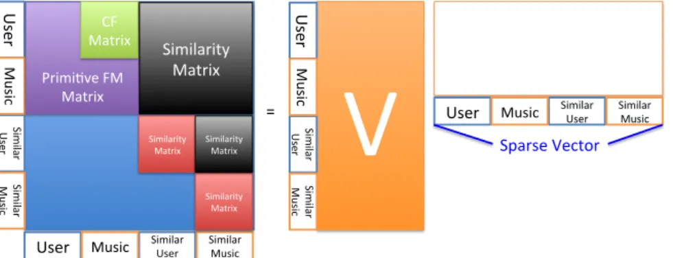
(26) to the standard factorization machine by grouping the features with similar characteristic. Therefore it can deal with the tasks in a more flexible way with different feature partitions. After removing the non-informative weights from the FM models, the original formula can be rewritten as: yˆ(x) = w0 +. n X. w i xi +. n X. n X. j2G(i) j 0 2G(i) /. i. xj xj 0.  X. vj,f vj 0 ,f ,. (3.3). f =1. where index i belongs to the same group G(i). The mutual effect of xj and xj 0 is dropped out under the setting. By the grouping technique, it eliminates the unnecessary interactions such as the interaction between a user and the user’s age is non-informative. From the perspective of technical part, the grouping technique not only speeds up the convergence of optimization but also provides a flexible way to construct different feature combinations. Note that the modified prediction function would be the same as the original. 政治大 LibFM provides three major 立立optimization criteria to learn the data: Stochastic Gradi-. one when every feature has its own group.. ent Descent [20] (SGD), Alternating Least-Squares [21] (ALS) and Markov Chain Monte. •‧ 國. ㈻㊫學. Carlo [19] (MCMC). In our experiments, the MCMC method is chosen because it can automatically learns the data without giving the learning rates and the regularization terms.. •‧. For MCMC, the gradient for the grouping Factorization Machine is derived as follows: 8 > > > <. y. sit. io. n. al. 3.3. (3.4). er. Nat. 1, if ✓ = w0 @ yˆ(x) h✓ (x) = = xj , if ✓ = wj > @✓ > > : x P0 vj 0 ,f xj , if ✓ = vj,f j j 2G(j) /. Ch. engchi Similarity Framework. i n U. v. Motivated by the strength and efficiency of CF method, we seek to combines the advantages with the factorization model. Since FM has a good framework for modeling the input features, we can directly extract the similarity information from the users and items. This way has the similar concept of CF method, and can be easily embedded into a feature vector. In general, the utilized features are divided into following three types, and each type has its own computation method. Figure 3.1 illustrates the main concept of incorporating similarity information into the FM framework. In general, a traditional CF-based matrix only keeps the records of user-to-item information, but FM factorizes this form to a multiplication of two feature vectors (i.e. V and V T in Figure 3.1). This way allows high-quality parameters estimated by higher-order interactions under sparsity. 1. ID Domain: The ID variable is used to identify a target, and it only belongs to a specific target. For instance, User ID is in the ID domain, which means that each 10.

(27) = Similarity! Matrix. Similarity! Matrix. Similar! User!. User! Music!. Similar! User!. Similar! Music!. Sparse!Vector!. Similar! Music!. Similar! Music!. Similarity! Matrix. User! Music!. T V. V. Similar! User!. Similar! User!. !. Similarity! Matrix. ! !. User! Music!. User! Music!. ! CF! ! Matrix ! Primi2ve!FM! Matrix. Similar! Music!. 立立. 政治大. Figure 3.1: Factorization Machine with similarity framework. •‧ 國. ㈻㊫學. user has his/her own unique ID variable. Technically a similarity measurement is a function that computes the degree of similarity between a pair of targets, e.g. the. •‧. similarity of listening histories of two users. Here we apply an extended version of. n. al. y. O(Ti ) \ O(Tj ) , |O(Ti )|1 ↵ |O(Tj )|↵. (3.5). er. io. sij =. sit. Nat. cosine similarity as our measurement:. where ↵ 2 [0, 1] is a tuning parameter.. Ch. engchi. i n U. v. 2. Categorical Domain: The categorical variable represents the extracted features from the user and item attributes such as the User Age and Music Genre. The similarity computation is also based on Equation (3.5).. 3. Real Value Domain: If the attribute is already a number 2 R, such as Audio Information. The similarity score is calculated by the Euclidean distance. In general, for an n-dimensional space, the distance between feature vector q and feature vector p is: d(p, q) =. v u n uX t (p. i. qi ) 2 .. (3.6). i=1. For the ID domain, the function O represents the referred objects from target i and target j. For example, given the listening histories of two users the ↵ determines whether 11.

(28) the similarity score considers the amount of referred objects from another target or not. Take the following three users with the listening records as an example: O(U seri ) = [1, 2, 3], O(U serj ) = [1, 2, 3], O(U serk ) = [1, 2, 3, 4]. Then U serj is more similar to U seri than U serk based on the listening history while the ↵ = 1; on the other hand, they will get a same score while the ↵ = 0. For the categorical indicators, because this kind of feature usually occurs in different objects, the function O will be the collection of referred objects for a target. Take the User Age as an example, if we want to know the similarity of listening history between. 政治大 users whose age is between 15 and 30. 立立 For the real-value indicators, the feature vector is normalized by the standard score: , where µ is the mean of the population and. ㈻㊫學. x µ. •‧ 國. 15-year-old users and 30-year-old users, the function O will collect all the songs of the. is the standard deviation of the popula-. tion. The score indicates how many standard deviations an observation is above or below. •‧. the mean.. Finally suppose we have a set of similarity scores for a specific target and seek to. sit. y. Nat. embed them into a feature vector, a simple way is to directly index them with corresponding scores. However, the popular object generally contains more similar objects than the. io. n. al. er. others. It may leads to an unbalance problem that unpopular objects are hard to get the. i n U. v. similarity score. In order to the balance issues into account, we only keep the top-k similar. Ch. engchi. objects as the new score basis, and normalize the new vector of k values to 1: sij . j 0 =1 |sij 0 |. s¯ij = Pn. (3.7). The purpose of this step is to avoid the unbalance of similarity information. For example, s(U seri ) = (0, 0.8, 0.6) and s(U serj ) = (0.1, 0, 0.2), U seri will have more probability of getting high scores because of the high values of the similarity vector.. 3.4. Extracted Features. The structure of collected music dataset is depicted in Figure 3.2. Personal factors indicate the characteristics that people would possess for a long period of time, such as age, gender. People with different levels of music background may appreciate music differently, which in turn affects music preference. Musical factors consist of the audio content, its profile, and even the artwork of the CD. People may choose a song because its melody 12.

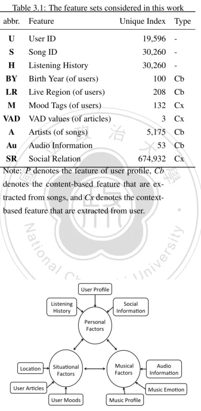
(29) Table 3.1: The feature sets considered in this work abbr.. Feature. Unique Index Type. U. User ID. 19,596. -. S. Song ID. 30,260. -. H. Listening History. 30,260. -. BY. Birth Year (of users). 100. Cb. LR. Live Region (of users). 208. Cb. M. Mood Tags (of users). 132. Cx. 3. Cx. VAD VAD values (of articles) A Au. 治 5,175 政大 53 Audio Information Social立立 Relation 674,932 Artists (of songs). Cb Cb. SR Note: P denotes the feature of user profile, Cb. Cx. •‧ 國. ㈻㊫學. denotes the content-based feature that are exbased feature that are extracted from user.. Nat. n. al. er. io. sit. y. •‧. tracted from songs, and Cx denotes the context-. Ch. engchi. User(Profile(. Listening( History(. i n U. v. Social( Informa4on( Personal( Factors(. Loca4on(. Situa4onal( Factors(. (Musical( Factors(. User(Moods(. Music(Profile(. User(Ar4cles(. Audio( Informa4on( Music(Emo4on(. Figure 3.2: The structure of LiveJournal dataset. 13.

(30) or the singer. Situational factors include those that persist for a short period time such as when and where you listen to music, what you are doing and what your mood is. People usually express their feelings though listening to music, and the user-generated article reflects their recent mood.The structure of collected music dataset is depicted in Figure 3.2, as these factors affect how people choose the music. Personal factors indicate the characteristics that people would possess for a long period of time, such as age, gender. People with different levels of music background may appreciate music differently, which in turn affects music preference. Musical factors consist of the audio content, its profile, and even the artwork of the CD. People may choos a song because its melody or the singer. Situational factors include those that persist for a short period time such as when and where you listen to music, what you are doing and what your mood is. People usually express their feelings though listening to music, and the user-generated article reflects their recent mood.. 立立. 政治大. Table 3.1 summarizes the features used in the experiments, which are described in. •‧. •‧ 國. ㈻㊫學. detail below.. er. io. sit. y. Nat. 3.4.1 Content-based Features. Content-based features refer to features that describe either the user or the item. For de-. n. al. i n U. v. scribing users, we have Birth Year (BY), Live Region (LR) and Social Relations (SR). Ch. engchi. features. The birth years for the users in our dataset fall in a window of 100 years. Moreover, the users are from 208 regions. We consider users who were born in the same year or users who were from the same region as similar. On the other hand, from LiveJournal we can obtain social information regarding who is who’s friend and construct the social network among the users. This gives rise to the social relation based similarity matrix. People who are friends to one another are likely to share similar music taste. For describing songs, we have Artist (A) and Audio Information (Au) features. The artist feature simply indicates the artist (among the 5,175 possible artists) of the songs. If two songs are sung/performed by the same artist, they are likely to be more similar. The audio features consists of 53 perceptual dimensions of music, including danceability, loudness, key, mode, tempo, pitches and timbre, with a total of 53-Dimensions. They are extracted by using the EchoNest API 1 , a commonly used audio feature extraction tool developed in the field of music information retrieval [9]. We can measure the similarity between two songs in this 53-dimensional feature space. 14.

(31) Table 3.2: Affective Norms for English words: 5 example words Description Valence Arousal Dominance dream. 6.73. 4.53. 5.53. eat. 7.47. 5.69. 5.60. favor. 6.46. 4.54. 5.67. good. 7.47. 5.43. 6.41. hate. 2.12. 6.95. 5.05. 3.4.2 Context-based Features The user-generated articles are interesting context-based features in the dataset, but it. 政治大. may contains too many redundant words. Motivated by the idea of emotional matching, we convert the original content of an article into a vector of emotional words by referring. 立立. to the dictionary of Active Norms for English Words (ANEW) [4], which provides a set of. •‧ 國. ㈻㊫學. normative emotional ratings for English words. There are totally 2,476 emotional words in ANEW, and there are about 3% of articles discarded, because they have no ANEW words. We leave the words which can be found in the ANEW dictionary and weight them. •‧. n. idf (t, d) = log. Ch. sit. io. al. f (w, d) , max{f (w, d) : w 2 d} |D| , |{d 2 D : t 2 d}|. er. Nat. tf (t, d) =. y. by the TF-IDF weighting. Specifically, a word is scored by tf (t, d) ⇥ idf (t, d), where. engchi U. v ni. (3.8) (3.9). and D is the total number of articles. A term with the high score indicates that the term has a higher term frequency wight and a lower document frequency of the term in the whole collection of articles. In addition, the ANEW dictionary also provides a set of normative emotional ratings for English words. The emotional words are rated by Valence (or pleasantness; positive/negative active states) , Activation (or arousal; energy and stimulation level) and Dominance (or potency; a sense of control or freedom to act), the fundamental emotion dimensions found by psychologists [9]. Finally each word vector of articles is converted to valence, arousal, and dominance (VAD) values. For example, for the sentence ”I had a dream last night, I was eating a marshmallow,” the VAD values would be 14.2, 10.22, and 11.13, respectively, according to Table 3.2. Moreover, we also collected the recent mood tags which are recent used by each user.. 1. http://echonest.com/. 15.


(33) Chapter 4 Experimental Results 4.1 Experimental Settings. 政治大. 立立. 4.1.1 Dataset. •‧ 國. ㈻㊫學. Our experiments are performed on a real-world dataset collected from a commercial websites – LiveJournal 1 . LiveJournal is a well-known social blogging website where users. •‧. listen to music while writing their online diaries. LiveJournal is unique in that, in addition to the common feature of blogging, each post is accompanied with a ”Mood” column and. Nat. sit. y. a ”Music” column so that users can write down their moods and songs in their minds while posting, as Figure 4.1 exemplifies. From LiveJournal, we crawled a total number. io. n. al. er. of 1,928,868 listening records covering 674,932 users and 72,913 songs as an initial set.. i n U. v. For the purpose of retaining enough number of data in the training and test sets for this. Ch. engchi. study, we only considered users who have more than 10 listening records and discarded the records of the other users. This filtering resulted in the final set of 225,652 listening 1. http://www.livejournal.com/. Figure 4.1: Livejournal sample posts 17.

(34) records (11.7% of the initial set) among 19,596 users and 30,260 songs. For evaluation, we split the dataset for each user according to the following 80/20 rule: keeping full listening history for the 80% and the half of listening history for the remaining 20% users as the training data, and the missing half of the remaining 20% users as the testing data. For each recorded song, we randomly add 10 songs as negative records to construct the testing pool.. 4.1.2 Evaluation Metrics We employed two metrics to evaluate the recommendation performance: the truncated mean average precision at k (MAP@k) and recall. For each user, let P (k) denotes the precision at cut-off k:. Pk. P (k) ⇥ ruo(p) , (4.1) I(u) where o(p) = i means the item i is ranked at position p in the order list o, and rui means. 政治大. AP (u, o) =. 立立. p=1. whether the user u has listened to song i or not(1 = yes, 0 = no). MAP@k is the mean. •‧ 國. ㈻㊫學. of the average precision scores for the top-k results: PU. AP (u, o) , (4.2) U where U is the total number of target users. Higher MAP@k indicates better recommenu=1. •‧. y. Nat. dation accuracy.. M AP @k =. sit. Recall measures how many songs the user really likes are recommended by the auto-. n. al. er. io. matic system. It is computed by: Recall =. i n U. v. |{Correct Songs}| \ |{Returned T op k Songs}| . |{Correct Songs}|. Ch. engchi. (4.3). High recall means that most of songs the user actually likes or listens to are recommended. In the case of diversity, our evaluation metric is to check out the proportion of categories that appears in top-n recommendations. We define the diversity score as following formula: Coverage =. {number of unique categories in recommendations} . {total number of the categories}. (4.4). Therefore high score means the recommendations can cover a more wide range of music, and low score means the recommendations only focus on few specific domains of music.. 4.2 Contextual Recommendation System This section we focus on presenting the work of how to model the relationship between user’s mood and user’s listening behavior. To enhance the benefits from different perspective of features, we 18.

(35) 4.2.1 CF-based Recommendations Our first evaluation focuses on the use of CF information only for music recommendation. We compare FM with the following three well-know CF methods: user-based CF, itembased CF, and a SVD-based approach. Below we describe the main ideas of the methods. • User-based CF: This method weights all users with respect to their similarity to each other, and selects a subset of users (who are highly similar to the target user) as neighbors. It predicts the rating of specific song based on the neighbors’ ratings. Let S(u) be the set of songs that are chosen by the user u. The similarity between user u and user v is calculated by following formula: suv =. S(u) \ S(v) |S(u)|↵ |S(v)|1. ↵. (4.5). ,. 政治大. where ↵ 2 [0, 1] is a parameter to tune.. 立立. •‧ 國. ㈻㊫學. • Item-based CF: This method is similar to the user-based CF method. It computes. the similarity between songs and scores a song based on user’s listening history. The song similarity is calculated as follows: ↵. ,. (4.6). y. Nat. U (i) \ U (j) |U (i)|↵ |U (j)|1. •‧. sij =. io. sit. where U (i) the set of the users who have listened to the song i.. n. al. er. • SVD++: This method is an extended version of SVD-based latent factor models by. i n U. v. integrating implicit feedback into the model. In specific, the prediction formula can be the following:. Ch. engchi. rui = µ + bu + bi +. qiT. 0. @p u. +q. 1 |N (u)|. ⇥. X. j2N (u). 1. yi A ,. (4.7). where N (u) is the set of implicit information, µ is the global mean rating, bu is a scalar bias for user u, bi is a scalar bias for item i, pu is a feature vectors for user u, qi is a feature vector for item i. According to the results reported in the MSD Challenge [3], we set the ↵ in userbased CF and item-based CF to 0.5. Table 4.1 lists the preliminary results of MAP@10 and recall. As the table shows, the performance of all the implemented methods, except for the random baseline, seems to be reasonable, achieving about 0.30 to 0.38 in terms of MAP. Among the four methods, FM obtains the highest performance, showing that FM can be a competitive framework for this task. We therefore focus on the use of FM hereafter. 19.

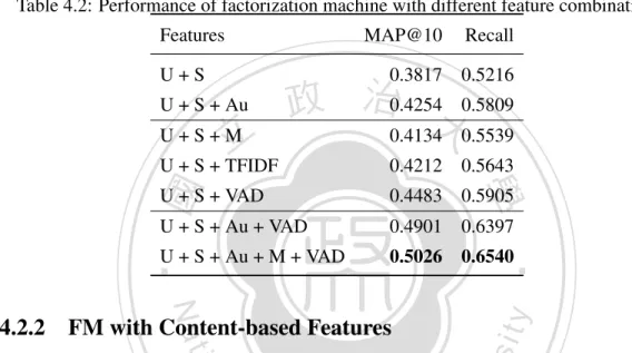
(36) Table 4.1: Evaluation result of CF-based algorithms Model. MAP@10. Recall. Randomize. 0.0578. 0.1656. User-based CF 0.3668. 0.4748. Item-based CF. 0.3093. 0.5115. SVD++. 0.3506. 0.4844. FM. 0.3817. 0.5216. Table 4.2: Performance of factorization machine with different feature combinations Features. MAP@10. Recall. 0.3817. 0.5216. 0.4212. 0.5643. U + S + VAD. 0.4483. 0.5905. U + S + Au + VAD. 0.4901. 0.6397. U + S + Au + M + VAD. 0.5026. 0.6540. 立立. U+S+M. 政治0.4254大0.5809 0.4134 0.5539. •‧. Nat. 4.2.2 FM with Content-based Features. ㈻㊫學. •‧ 國. U + S + TFIDF. y. U + S + Au. io. sit. U+S. er. Next, we evaluate the performance of content-based recommendation. It has been well. al. n. v i n C users are considered. that occurs when new items and new h e n g c h i U The problem can be alleviated known that the CF-based approach usually suffers from the so-called ”cold start” problem. by adding some content-based features, making it possible to recommend a new song by comparing its audio information to the audio information of other songs. As shown in the first two rows of Table 4.2, the content-based method (i.e., U + S + Cb) outperforms the CF-based one (i.e., U + S) by a great margin.. 4.2.3 FM with Content-based and Context-based Features We evaluate the performance of context-based recommendation by using Mood Tags and VAD, both represent the users’ mood. As shown in the third and fourth row of Table 4.2, the performance of adding the Mood Tags feature is improved from 0.3817 to 0.4134 in terms of MAP@10. This result shows that the contextual users’ mood information indeed improves the performance of recommendation. With the another contextual VAD feature from user-generated context, the performance is even higher, with the MAP@10 attaining 0.4483. This result implies that the VAD feature provides more emotional information of 20.

(37) Table 4.3: Performance of user similarity and item similarity LiveJournal Dataset Features. MAP@10. Recall. U+S. 0.3816. 0.5217. U+S+H. 0.4409. 0.5821. U + S + US. 0.4310. 0.5712. U + S + H + US. 0.4427. 0.5810. U + S + SS. 0.4635. 0.6194. U + S + H + SS. 0.4897. 0.6413. U + S + US + SS. 0.4712. 0.6251. U + S + US + SS + H 0.5021. 0.6491. 政治大. Note: For the feature abbreviation, please refer to Table 3.1.. 立立. the user context, which might not be easily captured by mood tags only.. •‧ 國. ㈻㊫學. Finally, we evaluate the hybrid model that combines the two contextual features and the content-based features (i.e., U + S + Cb + M + VAD). As the last row of Table 4.2. •‧. shows, this hybrid model greatly outperforms the content-based method, achieving 0.50 and 0.65 in terms of MAP and recall, respectively. The performance difference between. y. Nat. the hybrid model and the CF-based or content-based models are significant under the two-. sit. tailed t-test (p-value< 0.001). On the other hand, we also provide an experimental result. er. io. that without using the user-provided Mood tags (i.e., U + S+ Au + VAD). By comparing it. al. v i n C hcontextual information experimental results suggest that the i U mined from user-generated e h n c g articles improves the quality of music recommendation. n. to purely hybrid CF+CB method, we still see great performance improvement. In sum, the. 4.3. Similarity Approach. The similarity indicator can be represented as the categorical set domain as used in [21]. For instance, suppose that ”Alice is similar to Charlie and Sandy”, the corresponding similarity indicator may be the vector z(Bob, Charlie, Sandy) = (0, 0.2, 0.8), where the sum of all values equals to 1 according to Equation (3.7). Below we investigate the effectiveness of similarity information under different types of extracted features.. 4.3.1 User Similarity and Item Similarity Under the CF-based framework, there are two ID indicators: User ID and Song ID. We can obtain the following similarity information according to Equation (3.5): 21.

(38) • User Similarity (US): Two users are similar if they listen to same songs. • Song Similarity (SS): Two songs are similar if they are listened by same users. Both of them are directly mined from the listening history. Therefore, they are always available for a standard recommendation problem. US is applied to users, whereas the SS is applied to items. We evaluated the performance on every possible feature combination. As shown in Table 4.3, both the user similarity and the song similarity (U+S+US or U+S+SS) lead to significantly better result, comparing to the baseline U+S. We have also implemented KNN-based FM of [1] by adding the listening history to libFM, as can be seen from the second row of Table 4.3 (i.e., U+S+H). It can be seen that the incorporation of listening history (‘H’) generally improves the result as well. If. 政治大 the similarity approach is more effective than the KNN approach does. Unlike listening 立立 history, similarity is extracted by a meaningful computation. Moreover, KNN approach. we compare H, US, and SS, SS achieves the highest MAP@10 (0.4635), showing that. •‧ 國. ㈻㊫學. may fails when the amount of listening history is limited.. By combining all the available information from the listening records (U+S+US+SS+H),. •‧. we obtained the best result 0.5021 in MAP@10 in Table 4.3, which is significantly better than the baseline 0.3816. It should be noted this result indicates an improvement in. sit. y. Nat. MAP@10 by more 0.1205, which is a very remarkable improvement. A simple idea as it is, using the proposed ID similarity indicators holds the promise of greatly improv-. io. n. al. er. ing the accuracy of recommendation. Moreover, the ID similarity indicators are suitable. i n U. v. for other recommendation problems because they are in the same problem structure: to. Ch. engchi. predict whether an item would be accepted by a user.. 4.3.2 Content-based feature similarity With regard to content-based feature, there are four similarity features were extracted from the dataset: • Birth Year Similarity (BYS): Two users are similar if they are born in the same year.. • Live Region Similarity (LRS): Two users are similar if they live in the same region geographically.. • Artist Similarity (AS): Two songs are similar if they are sung by the same artist. • Audio Similarity (AuS): Two songs are similar if they are close in the audio feature space spanned by the 53 audio features considered in this work. 22.

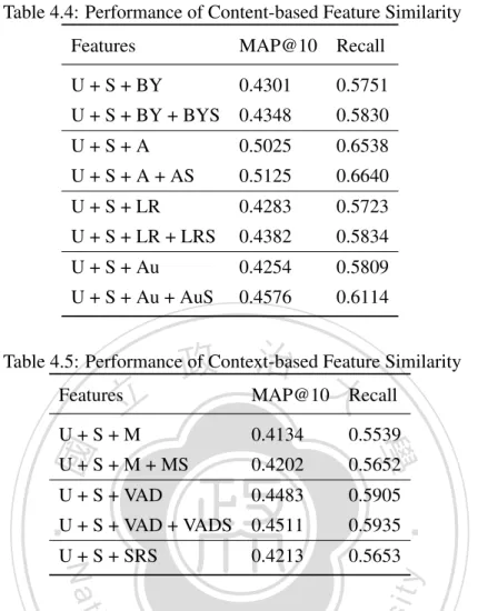
(39) Table 4.4: Performance of Content-based Feature Similarity Features. MAP@10 Recall. U + S + BY. 0.4301. 0.5751. U + S + BY + BYS 0.4348. 0.5830. U+S+A. 0.5025. 0.6538. U + S + A + AS. 0.5125. 0.6640. U + S + LR. 0.4283. 0.5723. U + S + LR + LRS. 0.4382. 0.5834. U + S + Au. 0.4254. 0.5809. U + S + Au + AuS. 0.4576. 0.6114. 政治大 MAP@10 Recall. Table 4.5: Performance of Context-based Feature Similarity Features. 立立. 0.5539. U + S + M + MS. 0.4202. 0.5652. U + S + VAD. 0.4483. 0.5905. U + S + VAD + VADS 0.4511. 0.5935. U + S + SRS. 0.5653. sit. y. Nat. 0.4213. •‧. •‧ 國. 0.4134. ㈻㊫學. U+S+M. er. io. Note that BYS and LRS are personal information that is not always available for a recom-. al. v i n Cthe if we have access to the metadata or content ofUthe songs. h eaudio n chi g Table 4.4 lists the improvement introduced by the use of feature similarity. The results n. mendation problem. Similarly, AS and Aus are musical information that is only available. show that four similarities perform well in recommendations. Among the four similarities, Birth Year Similarity cannot obtain a significant improvement in the experiments. This is possibly due to incompleteness of the metadata, because only half users have birth year information in our dataset. Moreover, another interesting observation is that the audio feature has a great enhancement on the recommendation performance after the audio similarity is added. The result implies that the abstract information such as the audio feature is hard to be organized directly, but its similarity information provides insightful information.. 4.3.3 Context-based feature similarity We evaluated context-based recommendations by using Mood Tag and Emotional Words. These two features reflect the user’s mood when writing the article. We want to carry 23.

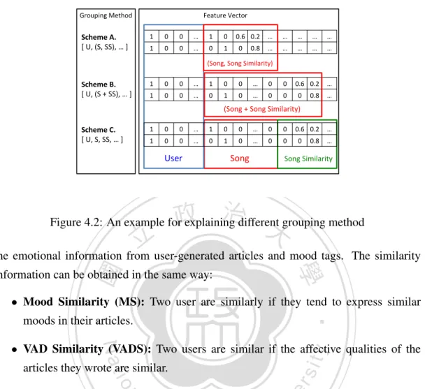
(40) Grouping"Method". Feature"Vector". Scheme&A.& ["U,"(S,"SS),"…"]". 1". 0". 0". …". 1". 0" 0.6" 0.2" …". …". …". …". …". 1". 0". 0". …". 0". 1". …". …". …". …". 0" 0.8" …". (Song,"Song"Similarity)". Scheme&B.& ["U,"(S"+"SS),"…"]". 1". 0". 0". …". 1". 0". 0". …". 0". 0" 0.6" 0.2" …". 1". 0". 0". …". 0". 1". 0". …". 0". 0". 0" 0.8" …". (Song"+"Song"Similarity)" Scheme&C.& ["U,"S,"SS,"…"]". 1". 0". 0". …". 1". 0". 0". …". 0". 0" 0.6" 0.2" …". 1". 0". 0". …". 0". 1". 0". …". 0". 0". User". Song". 0" 0.8" …". Song"Similarity". 政治大. Figure 4.2: An example for explaining different grouping method. 立立. the emotional information from user-generated articles and mood tags. The similarity. •‧ 國. ㈻㊫學. information can be obtained in the same way:. •‧. • Mood Similarity (MS): Two user are similarly if they tend to express similar moods in their articles.. sit. y. Nat. • VAD Similarity (VADS): Two users are similar if the affective qualities of the. io. al. er. articles they wrote are similar.. n. Please note that contextual information is also an advanced feature that is not always avail-. Ch. i n U. v. able for a recommendation problem. However, whenever it is possible to model context. engchi. information, it is usually advisable to do so. We only considered context information extracted from mood tags and articles in this work, but it should be noted that the proposed method applies to other contextual information as well. As the first and third rows of Table 4.5 shows, the performance of adding the Mood Tags feature is 0.4134 in terms of MAP@10, which is higher than the contextual VAD feature computed from user-generated articles. This result indicates that the VAD feature provides more affective information of the user context. Although the mood similarity does not lead to remarkable improvement, the VAD similarity feature is still considered effective.. 4.4. Grouping Approach. Since there are too many similarity features, some interactions might be non-informative. Taking the following situation as an example: ”Alice is similar to Charlie and Sandy;” it 24.

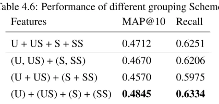
(41) Table 4.6: Performance of different grouping Scheme Features MAP@10 Recall U + US + S + SS. 0.4712. 0.6251. (U, US) + (S, SS). 0.4670. 0.6206. (U + US) + (S + SS). 0.4570. 0.5975. (U) + (US) + (S) + (SS) 0.4845. 0.6334. does not mean Charlie is similar to Sandy. For this reason, we applied grouping Factorization Machine as an extended model to offer a more flexible framework for combining the features. Since the self-group interactions are eliminated from the model, we have more choices to build different useful features. Specifically, we employed following three. 政治大. grouping schemes for the indexing method of similarities: • Same Group and Same Index. 立立. •‧ 國. ㈻㊫學. • Same Group and Different Index • Different Group and Different Index. •‧. Figure 4.2 illustrates the three grouping schemes. The scores of similar songs will be directly added in the same indexes for the first scheme, but will have additional index. Nat. sit. y. value in the second scheme. Scheme A can reduce the index dimension, but it is inappropriate for combing multiple features since the index may encounters the duplication prob-. io. n. al. er. lem. For the third scheme, the song similarities are indexed in another group. The main. i n U. v. difference is that the interactions between the song and similar songs will be counted in. Ch. engchi. learning process. In short, the feature vector can be organized with more different forms. We evaluated the three schemes on user-item features with the grouping factorization machine. Table 4.6 shows the result. The first result is conducted by standard factorization machine and the remaining results are obtained from the grouping factorization machine. We suggest that the interactions between object and similar objects are helpful according to the performance, but the noise may occurs when the interactions between similar features. In view of this, we adopt the grouping factorization machine as an extended method to further improve the quality of recommendations. The final result is shown in Table 4.7. Moreover, in order to demonstrate the strength of grouping factorization, we further examine performance on the standard factorization machine with different settings.. 4.4.1 Training Loss Figure 4.3 plots the training loss in the training step of the two approaches. The Y-axis corresponds to the root mean square error (RMSE), measuring the difference between 25.

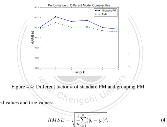
(42) Training loss of Training Data. 0.25. FMs GroupingFM 0.24. RMSE. 0.23. 0.22. 0.21. 0.20. 0. 20. 40. 60. Iteration. 80. 100. 120. Figure 4.3: Training loss between standard FM and grouping FM. 政治大. Performance of Different Model Complexities. 0.530. GroupingFM FMs. 立立. 0.525. 0.520. MAP@10. •‧ 國. ㈻㊫學. 0.515. •‧. 0.510. 0.505. y. Nat. 5. io. al. 6. Factor k. 7. 8. 9. sit. 4. er. 0.500. v. n. Figure 4.4: Different factor  of standard FM and grouping FM predicted values and true values:. Ch. engchi. RM SE =. v u n u1X t (yˆ. n i=1. i. i n U. yi ) 2 .. (4.8). The X-axis indicates the number of iterations. Obviously, the grouping factorization machine is much fast to achieve the convergence. In addition, although it dose not get a lower RMSE score, it still gets a better generalized performance on testing data. In other words, the grouping action helps prevent the model from overfitting the training data.. 4.4.2 Model Complexity We changed the parameter  from 3 to 10, and plotted the performance in Figure 4.4. The grouping factorization machine gets better performance for each factor . The results indicate that the grouping FM is useful to enhance the quality of recommendations. 26.

(43) Table 4.7: Performance on complete feature vector Features MAP@10 Recall Note U+S. 0.3817. 0.5216. U + S + C*. 0.5120. 0.6614. U + S + C* + S*. 0.5236. 0.6684. Base-line Hybrid. U + S + C* + S* 0.5251 0.6708 Hybrid + Grouping Note: C* denotes all the categorical features, and S* denotes all the extracted similarity features. Table 4.8: Coverage scores with top-k similarity information Features Coverage U+S+K. 0.477. U + S + K + top-5 similar Ks. 0.470. U + S + K + top-7 similar Ks. 0.466. U + S + K + top-9 similar Ks. 0.537. ㈻㊫學. •‧ 國. 政similar治Ks 0.222 U + S + K + top-1 大 U + S立立 + K + top-3 similar Ks 0.261 •‧ sit. y. Nat. 4.4.3 Hybrid Recommendations. er. io. We studied if we can further boost the accuracy by integrating all the proposed similarity features, including categorical ones (denoted as C* collectively) and similarity features. n. al. i n U. v. (denoted as S* collectively). As Table 4.7 shows, using more data generally leads to bet-. Ch. engchi. ter accuracy. When all the features are considered (U+S+C*+S*), we are able to obtain 0.5251 in MAP@10 and 0.6708 in recall, both of which are the highest ones in our evaluation. This result confirms again the ability of the proposed method in incorporating multiple similarity information.. 4.5. Recommendation Diversity. Every user has his/her own habit of music listening. In other words, the motivation of choosing a type of music to listen to may depends on user’s mood, the weather or the occasion. That is why we generally consider the utilized features as more as possible while building the recommender system. From a different perspective to handle the problem, some users may want to discover the musics they never know before. Base on such situation, we seek to investigate the recommendation diversity in this section. The goal is to recommend the diverse songs to the user who only focus on specific domain of music. 27.

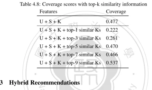
(44) 0.6. Coverage. 0.5. based-line. 0.4. 0.3. 0.2. 0.1. 0.0. k=1. k=3. k=5 k=7 Top-k similarity information. k=9. Figure 4.5: Recommendation diversity with top k similarity information. 政治大 information. Consequently, all the musics are partitioned into 10 clusters according to 立立 the 53-dimensional audio feature. The clustering results are denoted as K in our exper-. In our experiments, the basis of diversity rests on a k-means clustering result of audio. •‧ 國. ㈻㊫學. iments. Finally, we filter out the users who already listened to various clusters, because our objective is to help the users discovering the types of song they never listen to before.. •‧. Similarity and Diversity are two sides of one thing. By integrating different numbers of similarity information, our proposed method is able to control how diverse the rec-. y. Nat. ommended musics are. Table 4.8 lists the coverage scores while different numbers of. sit. similarity information had been considered. The result show that we build the recom-. er. io. mendation results with coverage score from 0.19 to 0.55. Moreover, the lower amount. al. n. v i n of similarity information we user,C the hhigher e n gcoverage c h i Uscore we get.. of similarity information we use, the lower coverage score we get. The higher amount As the growth of. similarity information, the proposed method is able to find out more domains of music. Figure 4.5 can help us finding the tendency via comparing to the base-line result (i.e., U + S + C). It implies that controlling the number of similarity information can indirectly control the recommendation diversity.. 28.

(45) Chapter 5 Conclusions In this paper, we have presented a novel approach that incorporates multiple feature simi-. 政治大 the similar patterns from the objects and enhances the convergence speed and accuracy of 立立 FM. The proposed method is applicable to many kinds of features, which means we can larity to factorization model via feature engineering. The similarity computation captures. •‧ 國. ㈻㊫學. obtain the higher level information from multiple aspects. Our experimental results show that feature similarity indeed benefits the recommendation performance. We also pro-. •‧. pose several features, including CF-based, content-based and context-based ones. Among these features, we try to capture the relationship between users and songs by matching. sit. y. Nat. users’ emotions. The results show that the idea is able to enhance the quality of recommendations. Moreover, by integrating different number of similarity information, we are. io. n. al. er. capable of controlling how diverse the recommendations are. Then, in order to avoid the. i n U. v. noise within large similarity features, we adopt the grouping FM as the extended method. Ch. engchi. to model the problem. The unnecessary connection can be eliminated if the features are within a same group. With the aforementioned technical contributions, we are able to improve the Mean Average Precision in music recommendation for a real-world, large-scale dataset from 0.3817 to 0.5251, comparing to the tradition CF-based baseline. In addition, via combing different number of similarity information, we can make the prediction results from 0.19 to 0.55 in terms of Coverage. Diversity becomes an important issue for real-world Recommendation Systems. Although our proposed similarity features can diversify the prediction results, to go one step further, we seek to start the work from the core of model. That is, we are looking forward about developing a recommendation model that is capable of generating a diverse recommendation list without feature engineering.. 29.


(47) Bibliography [1] Factorization machines with libfm. ACM Trans. Intell. Syst. Technol., 3(3):57:1– 57:22, May 2012. [2] R. Agrawal, S. Gollapudi, A. Halverson, and S. Ieong. Diversifying search results. In Proceedings of the Second ACM International Conference on Web Search and. 政治大. Data Mining, WSDM ’09, pages 5–14. ACM, 2009.. 立立. [3] F. Aiolli. A preliminary study of a recommender system for the million songs dataset. •‧ 國. ㈻㊫學. challenge. In Proceedings of the ECAI Workshop on Preference Learning: Problems and Application in AI, 2012.. •‧. [4] M. Bradley and P. J. Lang. Affective norms for english words ANEW: Instruction. y. Nat. manual and affective ratings. Technical report, The Center for Research in Psy-. io. sit. chophysiology, Univ. Florida, 1999.. n. al. er. [5] R. Cai, C. Zhang, C. Wang, L. Zhang, and W.-Y. Ma. Musicsense: contextual. i n U. v. music recommendation using emotional allocation modeling. In Proceedings of the. Ch. engchi. 15th international conference on Multimedia, MULTIMEDIA ’07, pages 553–556. ACM, 2007.. [6] K. Chen, T. Chen, G. Zheng, O. Jin, E. Yao, and Y. Yu. Collaborative personalized tweet recommendation. In Proceedings of the 35th international ACM SIGIR conference on Research and development in information retrieval, SIGIR ’12, pages 661–670. ACM, 2012. [7] T. Chen, L. Tang, Q. Liu, D. Yang, S. Xie, X. Cao, C. Wu, E. Yao, Z. Liu, Z. Jiang, et al. Combining factorization model and additive forest for collaborative followee recommendation. [8] J. Davidson, B. Liebald, J. Liu, P. Nandy, T. Van Vleet, U. Gargi, S. Gupta, Y. He, M. Lambert, B. Livingston, and D. Sampath. The youtube video recommendation system. In Proceedings of the fourth ACM conference on Recommender systems, RecSys ’10, pages 293–296. ACM, 2010. 31.

(48) [9] D. T. Derek Tingle, Youngmoo E. Kim. Exploring automatic music annotation with acoustically-objective tags. pages 55–61, 2010. [10] N. Hariri, B. Mobasher, and R. Burke. Context-aware music recommendation based on latenttopic sequential patterns. In Proceedings of the sixth ACM conference on Recommender systems, RecSys ’12, pages 131–138. ACM, 2012. [11] L. Hong, A. S. Doumith, and B. D. Davison. Co-factorization machines: modeling user interests and predicting individual decisions in twitter. In Proceedings of the sixth ACM international conference on Web search and data mining, WSDM ’13, pages 557–566. ACM, 2013. [12] M. Jiang, P. Cui, R. Liu, Q. Yang, F. Wang, W. Zhu, and S. Yang. Social contex-. 政治大 Information and knowledge management, CIKM ’12, pages 45–54. ACM, 2012. 立立. tual recommendation. In Proceedings of the 21st ACM international conference on. •‧ 國. ㈻㊫學. [13] M. Jiang, P. Cui, F. Wang, Q. Yang, W. Zhu, and S. Yang. Social recommendation across multiple relational domains. In Proceedings of the 21st ACM international conference on Information and knowledge management, CIKM ’12, pages 1422–. •‧. 1431. ACM, 2012.. Nat. sit. y. [14] N. Koenigstein, G. Dror, and Y. Koren. Yahoo! music recommendations: modeling music ratings with temporal dynamics and item taxonomy. In Proceedings of the. io. al. n. 2011.. er. fifth ACM conference on Recommender systems, RecSys ’11, pages 165–172. ACM,. Ch. engchi. i n U. v. [15] Y. Koren. Collaborative filtering with temporal dynamics. In Proceedings of the 15th ACM SIGKDD international conference on Knowledge discovery and data mining, KDD ’09, pages 447–456. ACM, 2009. [16] G. Linden, B. Smith, and J. York. Amazon.com recommendations: Item-to-item collaborative filtering. IEEE Internet Computing, 7(1):76–80, Jan. 2003. [17] H. Ma, C. Liu, I. King, and M. R. Lyu. Probabilistic factor models for web site recommendation. In Proceedings of the 34th international ACM SIGIR conference on Research and development in Information Retrieval, SIGIR ’11, pages 265–274. ACM, 2011. [18] I. Pilászy and D. Tikk. Recommending new movies: even a few ratings are more valuable than metadata. In Proceedings of the third ACM conference on Recommender systems, RecSys ’09, pages 93–100. ACM, 2009. 32.

(49) [19] S. Rendle. Bayesian factorization machines. [20] S. Rendle. Factorization machines. In Proceedings of the 10th IEEE International Conference on Data Mining. IEEE Computer Society, 2010. [21] S. Rendle, Z. Gantner, C. Freudenthaler, and L. Schmidt-Thieme. Fast contextaware recommendations with factorization machines. In Proceedings of the 34th international ACM SIGIR conference on Research and development in Information Retrieval, SIGIR ’11, pages 635–644. ACM, 2011. [22] T. Sakai. Evaluation with informational and navigational intents. In Proceedings of the 21st international conference on World Wide Web, WWW ’12, pages 499–508. ACM, 2012.. 政治大 relevance. In Proceedings of the 34th international ACM SIGIR conference on Re立立 search and development in Information Retrieval, SIGIR ’11, pages 1043–1052.. [23] T. Sakai and R. Song. Evaluating diversified search results using per-intent graded. •‧ 國. ㈻㊫學. ACM, 2011.. [24] Y. Shen and R. Jin. Learning personal + social latent factor model for social recom-. •‧. mendation. In Proceedings of the 18th ACM SIGKDD international conference on. sit. y. Nat. Knowledge discovery and data mining, KDD ’12, pages 1303–1311. ACM, 2012.. io. [25] Y. Shi, A. Karatzoglou, L. Baltrunas, M. Larson, A. Hanjalic, and N. Oliver. Tfmap:. n. al. er. optimizing map for top-n context-aware recommendation. In Proceedings of the. i n U. v. 35th international ACM SIGIR conference on Research and development in infor-. Ch. engchi. mation retrieval, SIGIR ’12, pages 155–164. ACM, 2012. [26] J. Weston, C. Wang, R. Weiss, and A. Berenzweig. Latent collaborative retrieval. CoRR, abs/1206.4603, 2012.. 33.

(50)